A tiny GPT¶

A GPT is a stack of identical blocks that reads a text from left to right and, at every position, outputs a probability for each possible next token. Everything a large language model does at inference time rests on that one trained function, and the whole architecture fits on a page: a tokenizer, two embedding tables, causal self-attention, a small MLP, layer norms and residual connections. This page builds a decoder-only transformer from those parts. It tokenizes text with byte-pair encoding and compares token counts across languages, cuts a token stream into next-token training pairs, runs one forward pass of a micro model by hand, counts the parameters of a GPT-2 small sized model exactly with and without weight tying, checks the loss at initialization against ln V, and trains a two-million-parameter model on a public-domain novel on one CPU thread in about a minute and a half. Afterwards you will be able to write a GPT from scratch, predict its parameter count and its first loss before running it, and recognize the bugs that make such a model look better than it is. It builds on Backpropagation and Attention.

To run the code in this topic, install the base, deep and nlp groups: PyTorch trains the model and tiktoken provides GPT-2's tokenizer.

Intuition¶

A language model assigns a probability to every possible continuation of a text. Written token by token, the probability of a whole sequence is a product of next-token probabilities:

The probability of a sequence x1 to xm is the product over t of the probability of xt given all the tokens before it

A model that predicts the next token well is therefore a model of the whole text. Training shows the model a window of real text and asks it, at every position at once, for the probability of the token that actually comes next. The loss is the average of minus the natural log of those probabilities, in nats per token, and e to the power of the loss is the perplexity:

The loss is minus one over n times the sum over positions t of the log of the probability the model gives to the next token, and the perplexity is e to the power of the loss

A perplexity of 160 means the model is as uncertain as if it chose uniformly among 160 tokens. Three ideas make a GPT work:

Tokens. Text becomes a sequence of integers from a fixed vocabulary of subword pieces. Frequent words are single tokens; rare words and other scripts fall back to smaller pieces, down to single bytes, so nothing is ever out of vocabulary.
Attention with a causal mask. Each position builds its new representation as a weighted average of the positions before it, with weights it computes from the content. The mask forbids looking ahead, which is what lets one forward pass train all positions of a window at once: position t predicts token t + 1 without seeing it.
Residual blocks. Every block reads the current representation, computes a correction and adds it back. Information and gradients flow along this residual stream from the embeddings to the output, and each block only has to learn a refinement.

The model from token ids to the loss: token ids pass through the token embedding, the position embedding is added, the sum runs through L pre-norm blocks, a final layer norm and the output layer, a softmax turns the logits into probabilities and the cross-entropy compares them with the targets; a dashed amber line marks that the output layer and the token embedding are the same matrix when tied

The diagram follows the data from token ids to the loss. Every box between the embeddings and the final layer norm keeps one row of width d per position; only the output layer widens each row to one score per vocabulary token. The dashed line is weight tying, explained below.

One pre-norm block: X goes through layer norm 1 and causal multi-head attention, and the result is added to X; that sum goes through layer norm 2 and the MLP, and the result is added again; the orange residual stream runs from X past both branches to the output

Inside a block, both branches read a normalized copy of the residual stream and add their output to the stream itself. The orange path is never normalized, which is why deep stacks of these blocks train easily.

How it works¶

Notation¶

Matrices hold one position per row, as mini-batch matrices hold one example per row in Backpropagation. Weight matrices use the torch.nn.Linear.weight layout, rows are outputs, so a linear layer computes the input times the transposed weight plus a bias added to every row. The symbols:

V is the vocabulary size, T the context length (the number of positions the model has embeddings for) and n the length of the current input, at most T.
d is the model width, h the number of attention heads, dₕ = d / h the head width and L the number of blocks.
x1 to xn are the token ids, integers from 0 to V - 1; m is the number of tokens in a stream and Δ the stride between training windows.
E is the token embedding, V by d, whose row v is the vector of token v, and P the learned position embedding, T by d.
X is the residual stream, n by d. The formula images write the stream after block l with a superscript (l); in the text, X0 is the embedded input.
WQ, WK, WU and WO are the query, key, value and output projections of one block, each d by d, and Q, K and U are the queries, keys and values of one head, each n by dₕ. Values are usually written V, a letter this page keeps for the vocabulary size.
W1 (4d by d) and W2 (d by 4d) are the MLP weights, and γ and β the gain and bias of a layer norm.
M is the causal mask, n by n, and z the logits of one position, with p = softmax(z).

Byte-pair encoding¶

A tokenizer maps text to ids from a fixed vocabulary. Byte-pair encoding (BPE) builds the vocabulary from data. It starts with the 256 possible byte values as tokens, so any UTF-8 text can be represented, and cuts the training text into chunks, for GPT-2 roughly words with their leading space, numbers, runs of punctuation and runs of whitespace. Merges never cross a chunk boundary. Then it repeats three steps until the vocabulary has the size it wants:

Count every adjacent pair of tokens inside the chunks, weighted by how often each chunk occurs.
Merge the most frequent pair into a new token and give it the next free rank, 256, 257 and so on.
Replace every occurrence of the pair by the new token.

GPT-2 learned 50,000 merges on web text; with the 256 bytes and one special token, <|endoftext|> with id 50256, that gives V = 50,257.

Encoding new text replays the training order: within each chunk, start from single bytes and repeatedly merge the adjacent pair whose merged token has the lowest rank, until no adjacent pair is in the vocabulary. The rank of a token is its id. This is the whole algorithm inside tiktoken, and byte_pair_merge, a dozen lines of Python, reproduces tiktoken's output token for token.

Two consequences follow from the construction. The leading space belongs to the token, so " sing" in the middle of a sentence and "sing" at the start of a text are different tokens, and so are " Holmes" (one token) and " holmes" (two). And languages poorly represented in the merge data are split into short pieces, in the extreme into single bytes of a multi-byte character. Here is the sentence "The library opens at nine o'clock every morning." in eight languages, with its length in characters and UTF-8 bytes and its token count under GPT-2's tokenizer (gpt2) and two later ones with larger vocabularies (cl100k_base and o200k_base):

English: 48 characters, 48 bytes; 11, 10 and 10 tokens.
German: 47 characters, 48 bytes; 19, 14 and 11 tokens, 1.7 times the English count under gpt2.
Turkish: 40 characters, 45 bytes; 22, 16 and 15 tokens, 2.0 times.
Uzbek: 51 characters, 51 bytes; 24, 23 and 19 tokens, 2.2 times.
Russian: 50 characters, 93 bytes; 54, 26 and 15 tokens, 4.9 times.
Hindi: 34 characters, 90 bytes; 54, 37 and 13 tokens, 4.9 times.
Korean: 24 characters, 58 bytes; 47, 22 and 19 tokens, 4.3 times.
Chinese: 12 characters, 36 bytes; 24, 15 and 11 tokens, 2.2 times.

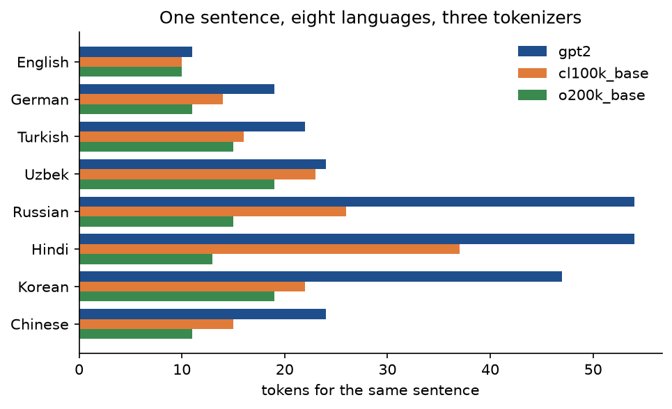
Token counts of the same sentence in eight languages under three tokenizers: blue bars for gpt2 reach 54 tokens for Russian and Hindi against 11 for English, while the orange cl100k_base and green o200k_base bars are much shorter for every non-English language

A context length is counted in tokens, and so is compute. Under GPT-2's tokenizer a Russian or Hindi text fills the same window with about a fifth of the content an English text does and costs five times as much to process; the larger vocabularies narrow the gap. Low-resource languages looks at what else changes for languages with little data, and Text processing at tokenization in general.

Training pairs from a sliding window¶

Tokenizing a corpus gives one long stream of ids s0 to s(m - 1). A window of length T starting at position i gives the input s(i) to s(i + T - 1) and, shifted one token to the right, the target s(i + 1) to s(i + T). Position t of the window is one training example: predict s(i + t + 1) from s(i) to s(i + t). Starting windows every Δ tokens gives

The number of windows is the floor of m minus T minus 1, divided by the stride, plus 1

windows, because the last target must exist. With Δ = T the windows tile the stream and every token is a target once; with a smaller stride they overlap and every token appears in about T / Δ windows. Split the stream into training and validation parts before cutting windows, never after (see Pitfalls).

Token and position embeddings¶

The first layer looks up one row of E per token and adds one row of P per position:

Row t of the embedded input is row x t of the token embedding plus row t of the position embedding, for t from 1 to n

A lookup is a matrix product with a one-hot vector, so E is an ordinary weight matrix trained by gradient descent. Without P the model could not tell positions apart: attention treats its inputs as a set, and permuting the input rows would just permute the output rows. GPT-2 learns P; the original transformer added fixed sinusoids, and recent models rotate queries and keys instead. A learned table has exactly T rows, so the model cannot take more than T tokens, and generation feeds it only the last T. The transformer architecture compares the positional schemes.

Causal multi-head self-attention¶

One head projects the normalized stream X to queries, keys and values, each with one row per position:

The queries are X times WQ transposed, the keys X times WK transposed and the values X times WU transposed

Position i scores every position j by the dot product of its query with j's key, scaled by the square root of the head width. The causal mask adds minus infinity to every score that looks ahead, a softmax turns each row of scores into weights, and the head output is the weighted average of the values:

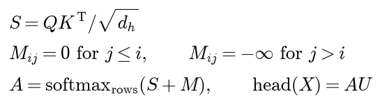
The scores are Q times K transposed divided by the square root of the head width; the mask is 0 on and below the diagonal and minus infinity above it; the attention weights are the row-wise softmax of the masked scores, and the head output is the weights times the values

Row i of A holds the attention weights of position i, non-negative and summing to one. Adding minus infinity before the softmax makes e to that power zero, so the future gets weight zero and the remaining weights still sum to one. Because row i of the output depends only on rows 1 to i of X, and every later layer acts on each position separately or through the same mask, the logits at position i depend only on x1 to xi. That is what makes it legitimate to compute the loss at all n positions in one pass.

The data flow of one attention head: the normalized stream is projected by WQ, WK and WU to queries, keys and values; queries and keys give the scaled scores; the amber causal mask is added and a row softmax gives the attention weights; the weights multiply the values, and the outputs of all heads are concatenated and projected by WO

The diagram shows the shapes: queries, keys and values are n by dₕ, the scores and weights n by n, and only after the heads are concatenated is the result n by d again.

The scaling keeps the softmax out of saturation. If the entries of a query and a key are independent with mean zero and variance one, their dot product is a sum of dₕ terms of variance one:

The variance of the dot product of q and k is the sum over the head width of the variances of the products, which is the head width; dividing by its square root brings the variance back to 1

Without the division, scores grow with the head width, the softmax approaches a one-hot vector and its gradient vanishes; tests/test_attention.py checks this on random vectors of width 256. Attention works through it by hand. With h heads, each head has its own projections of width dₕ, and the head outputs are concatenated and mixed by an output projection:

Multi-head attention concatenates the outputs of heads 1 to h and multiplies them by WO transposed, plus the bias bO

In code the h query projections are stacked into one d by d matrix, and likewise for keys and values; GPT-2 stacks all three into one 3d by d matrix with a bias and splits the result into heads by a reshape. The parameter count, 4d² + 4d per block, does not depend on h.

The pre-norm block¶

Layer norm standardizes each row over its d features with ε = 10⁻⁵ and then rescales it:

Layer norm of x is gamma times x minus mu, divided by the square root of sigma squared plus epsilon, plus beta, where mu is the mean of the d features and sigma squared their mean squared deviation

The MLP widens each position to 4d, applies GELU and projects back:

The MLP of U is GELU of U W1 transposed plus b1, times W2 transposed, plus b2; GELU of x is x times the standard normal distribution function of x, approximately one half x times 1 plus tanh of the square root of 2 over pi times x plus 0.044715 x cubed

Φ is the standard normal distribution function. GPT-2 uses the tanh form, which differs from xΦ(x) by at most 4.7 × 10⁻⁴, near x = -2.70 (tests/test_layers.py). A pre-norm block puts the normalization inside the residual branches:

A pre-norm block: X prime is X plus multi-head attention of layer norm 1 of X, and X double prime is X prime plus the MLP of layer norm 2 of X prime

The residual stream from X to X' to X'' is never normalized, so the derivative of the output with respect to the input contains an identity term from every block and gradients reach the embeddings undiminished. The original transformer normalized after the addition instead:

A post-norm block: X prime is layer norm 1 of X plus attention of X, and X double prime is layer norm 2 of X prime plus the MLP of X prime

That places a normalization on the main path of every block and makes deep stacks hard to train without a careful learning-rate warm-up. Because a pre-norm stream is never normalized, a pre-norm model needs one final layer norm after the last block. Each block also adds two branch outputs to the stream, so after L blocks the stream is a sum of 2L terms and its variance grows with L. GPT-2 compensates by drawing the two projections that write into the stream with a smaller standard deviation:

The output projection WO and the MLP contraction W2 are drawn with standard deviation 0.02 divided by the square root of 2L; every other matrix with 0.02

The 2L outputs added to the stream then have a combined variance that does not grow with the depth, and the stream keeps roughly the scale of the embeddings at initialization.

Output layer and weight tying¶

The final hidden state of position t becomes logits through one more matrix, Wout, of shape V by d, and a softmax turns the logits into probabilities. Wout has exactly the shape of E, and both relate tokens to the same d-dimensional space: E turns a token into a vector, Wout scores a vector against every token. Weight tying sets Wout = E:

The final hidden state is the final layer norm of the stream after block L; the logits are Wout times it and the probabilities their softmax; when tied, Wout equals E and the logit of token v is the dot product of row v of E with the hidden state

The logit of token v is the dot product of the hidden state with that token's own embedding. Tying saves Vd parameters, a quarter of GPT-2 small, and it changes how the embedding learns. Untied, row v of E receives a gradient only when token v appears in the input; tied, every row also receives a gradient from the softmax at every position, because the softmax pushes down every wrong token's logit (tests/test_torch_model.py checks both). GPT-2 ties its output layer. Tying means one tensor used twice, not two tensors and a footnote that subtracts one of them from the count.

Counting parameters¶

Per block, with all biases as in GPT-2, the two layer norms have 2d parameters each, the query, key and value projection 3d² + 3d, the attention output d² + d, the MLP expansion 4d² + 4d and the contraction 4d² + d:

Two d plus 3 d squared plus 3 d plus d squared plus d plus 2 d plus 4 d squared plus 4 d plus 4 d squared plus d equals 12 d squared plus 13 d

Adding the embeddings, the final layer norm and, if untied, the output layer:

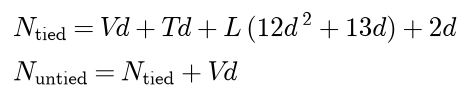
The tied count is V d plus T d plus L times 12 d squared plus 13 d, plus 2 d; the untied count adds another V d

For a check small enough to do in your head, V = 4, T = 3, d = 2 and L = 1 give 8 + 6 + (48 + 26) + 4 = 92 parameters tied and 100 untied. GPT-2 small has V = 50,257, T = 1,024, d = 768, h = 12 and L = 12; one block has 12 × 768² + 13 × 768 = 7,087,872 parameters. By group:

Token embedding Vd: 38,597,376.
Position embedding Td: 786,432.
Attention in the 12 blocks: 28,348,416.
MLP in the 12 blocks: 56,669,184.
The 25 layer norms: 38,400.
Output layer: none when tied, another 38,597,376 when untied.
Total: 124,439,808 tied and 163,037,184 untied.

The tied total is the size of the released GPT-2 small. examples/parameter_budget.py computes it three ways that must agree: the closed form above, the sum over the shapes the model is initialized with, and standard torch.nn layers (Embedding, Linear, LayerNorm) built on PyTorch's meta device, where parameters() yields the tied matrix once. Two thirds of a block is MLP. In a small model the embedding dominates instead: in the two-million-parameter model trained below, the tied token embedding is 58.7 % of all parameters.

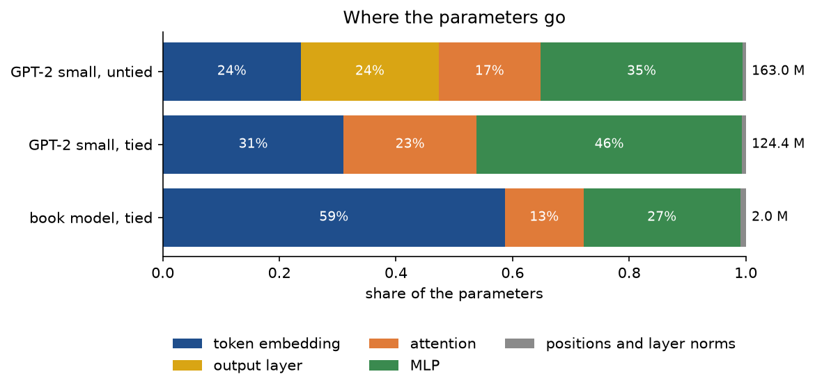
Share of the parameters by group for GPT-2 small untied, GPT-2 small tied and the book model: the token embedding and the output layer take about a quarter each of the untied GPT-2 small, the MLP dominates the tied GPT-2 small, and the token embedding takes 59 % of the book model

The three bars show why tying matters most for small models: the larger the vocabulary relative to the width, the larger the share of the parameters that sits in the embedding.

The loss at initialization¶

A model that knows nothing should spread its probability evenly, 1/V for every token, and score

The initial loss is minus the log of 1 over V, which is ln V

which is 10.8249 for V = 50,257. A freshly initialized model is close to this, and the size of the gap can be predicted. Suppose the logits of one position are independent draws from a normal distribution with standard deviation s, unrelated to which token is the target. Then

The expected initial loss is the expectation of the log of the sum of exponentiated logits minus the expected target logit, which is approximately ln of V times the expectation of e to the z, which equals ln V plus s squared over 2

using that a sum of V independent terms is close to V times their mean when V is large, and that the mean of e to the power z is e to the power s²/2 for a normal variable. The standard deviation s follows from the architecture. After the final layer norm with γ = 1 and β = 0, the hidden state has mean zero and variance one over its d entries, so its squared length is d, and each logit is its dot product with a row of weights of standard deviation 0.02:

The squared length of the hidden state is d; each logit is a weight row dotted with the hidden state, with weights drawn from a normal distribution with standard deviation 0.02, so s is 0.02 times the square root of d

For GPT-2 small s = 0.5543, s²/2 = 0.1536, and the expected first loss is 10.8249 + 0.1536 = 10.9785. On random token sequences examples/initial_loss.py measures 10.9787 for both the tied and the untied model, averaging minus the log probability over all 50,257 possible targets. On real text a tied model starts a little lower, because a token that already occurred in the context gets a slightly positive logit through the shared embedding, and real text repeats tokens. Whatever the details, a first loss far from ln V means a bug: a wrong vocabulary size, misaligned targets or an initialization that is far too large.

Choosing the next token¶

Generation runs the model on the prompt, turns the logits of the last position into a choice, appends it and repeats, cropping the input to the last T tokens. Greedy decoding takes the token with the largest logit. Sampling draws from the softmax of the logits divided by a temperature τ > 0:

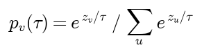
The probability of token v at temperature tau is e to the z v over tau divided by the sum over u of e to the z u over tau

A temperature below 1 sharpens the distribution towards greedy, above 1 flattens it towards uniform. Top-k sampling keeps the k largest logits, sets the rest to minus infinity and renormalizes. For the logits (1.5, 0.5, 0, -1):

τ = 0.5 gives the probabilities (0.8390, 0.1135, 0.0418, 0.0057).
τ = 1 gives (0.5977, 0.2199, 0.1334, 0.0491).
τ = 2 gives (0.4228, 0.2564, 0.1997, 0.1211).
τ = 1 with top-2 gives (0.7311, 0.2689, 0, 0).

Greedy decoding tends to fall into loops; plain sampling at τ = 1 occasionally picks a token from the long tail and derails. Decoding strategies covers these methods, beam search and nucleus sampling in depth, and Inference efficiency the key-value cache that avoids recomputing the prompt at every step.

Training¶

Training minimizes the loss over mini-batches of windows with AdamW, Adam with weight decay applied directly to the weights rather than through the gradient. Common choices for a small GPT, used below, are betas of 0.9 and 0.95, weight decay 0.1 on matrices but not on biases and layer norm parameters, gradients clipped to norm 1, and a linear warm-up to the peak learning rate followed by a cosine decay to a tenth of it over the remaining steps:

During the warm-up steps the learning rate is the peak times t plus 1 over the warm-up length; afterwards it is the floor plus half the difference between the peak and the floor times 1 plus the cosine of pi times the progress rho, where rho runs from 0 at the end of the warm-up to 1 at the last step

The warm-up keeps the first updates small while Adam's estimates of the gradient's scale are still poor, and the decay lets the model settle at the end. Gradients come from autograd; Backpropagation explains what it computes and Optimizers the update rules.

Worked example¶

Every value below is computed in double precision and rounded to four decimals for display. A hand calculation that rounds each intermediate result can differ in the last digit; where a sum written out below does, the text says so.

Tokens¶

Four BPE merges on the toy text "sing sing sings song sang", 25 bytes cut into the chunks "sing", " sing", " sings", " song" and " sang". At the start every token is a byte.

Rank 256 merges "n" and "g" into "ng". The pair occurs 5 times, once in each chunk; the runner-up is " " and "s" with 4.
Rank 257 merges " " and "s" into " s", 4 occurrences; the runners-up are "s" and "i", and "i" and "ng", with 3 each.
Rank 258 merges "i" and "ng" into "ing", 3 occurrences; the runner-up is " s" and "i" with 2.
Rank 259 merges " s" and "ing" into " sing", 2 occurrences; every remaining pair occurs once.

The four merges as a tree: the bytes n and g merge into ng with rank 256, space and s into space s with rank 257, i and ng into ing with rank 258, and space s and ing into space sing with rank 259, each labelled with its number of occurrences

The tree shows how each new token is built from earlier ones. After the four merges the text is 11 tokens: "s", "ing", " sing", " sing", "s", " s", "o", "ng", " s", "a", "ng". The first "sing" has no leading space and stays in two pieces.

Training pairs¶

GPT-2's tokenizer turns "Birds sing at dawn, and the valley wakes up." into 12 tokens: "B" (id 33), "irds" (11049), " sing" (1702), " at" (379), " dawn" (17577), "," (11), " and" (290), " the" (262), " valley" (19272), " wakes" (34267), " up" (510) and "." (13). "Birds" at the start of the text has no leading space and is not in the vocabulary as a whole word, so it splits. With T = 4 and Δ = 2 the formula above gives (12 - 4 - 1) / 2 = 3.5, rounded down to 3, plus 1: four windows.

Start 0: input "B", "irds", " sing", " at"; target "irds", " sing", " at", " dawn".
Start 2: input " sing", " at", " dawn", ","; target " at", " dawn", ",", " and".
Start 4: input " dawn", ",", " and", " the"; target ",", " and", " the", " valley".
Start 6: input " and", " the", " valley", " wakes"; target " the", " valley", " wakes", " up".

The first window alone holds four examples: "B" predicts "irds", "Birds" predicts " sing", "Birds sing" predicts " at" and "Birds sing at" predicts " dawn". The final "." is never a target, because a window starting at 8 would need a target at position 12.

One forward pass¶

A micro GPT with the vocabulary birds, sing, at, dawn (ids 0 to 3), context length T = 3, width d = 2, one attention head of width 2 and an output layer tied to the token embedding. It leaves out layer norm, the MLP and the output projection so that every number can be followed by hand. The input is "birds sing at", ids (0, 1, 2), with targets "sing at dawn", ids (1, 2, 3). The parameters, every matrix given row by row:

The token embedding E has rows birds (1, 0), sing (0, 1), at (-1, 0.5) and dawn (0.5, -1).
The position embedding P has rows (0, 0), (0.5, 0) and (0, 0.5).
WQ is the identity, with rows (1, 0) and (0, 1); WK has rows (1, 0.5) and (0, 1), so it adds half of the second feature to the first; WU has rows (0, 1) and (1, 0), so it swaps the two features.

The forward pass, one row per position:

Embedding. Rows 0, 1 and 2 of E plus the three rows of P give X with rows (1, 0), (0.5, 1) and (-1, 1).
Projections. Q equals X. K has rows (1, 0), (1, 1) and (-0.5, 1), and the values U have rows (0, 1), (1, 0.5) and (1, -1).
Scores. Q times K transposed, divided by √2, has rows (0.7071, 0.7071, -0.3536), (0.3536, 1.0607, 0.5303) and (-0.7071, 0, 1.0607). For example, position 2 against position 2 is (0.5 × 1 + 1 × 1) / √2 = 1.5 / 1.4142 = 1.0607.
Mask. Everything above the diagonal becomes minus infinity, so the masked rows are (0.7071, -inf, -inf), (0.3536, 1.0607, -inf) and (-0.7071, 0, 1.0607).
Attention weights. A row-by-row softmax gives (1, 0, 0), (0.3302, 0.6698, 0) and (0.1125, 0.2282, 0.6592). Position 1 can only attend to itself. For position 2 the exponentials of the two scores are 1.4241 and 2.8883, which add up to 4.3124.
Head output and residual. A U averages the value rows with these weights, giving (0, 1), (0.6698, 0.6651) and (0.8875, -0.4326), and adding X back gives H with rows (1, 1), (1.1698, 1.6651) and (-0.1125, 0.5674). The first entry of the third row of A U is 0.1125 × 0 + 0.2282 × 1 + 0.6592 × 1, which is 0.8874 from the rounded weights and 0.8875 at full precision.
Tied output layer. The logits are H times E transposed, each hidden row dotted with every token's embedding: (1, 1, -0.5, -0.5), (1.1698, 1.6651, -0.3372, -1.0802) and (-0.1125, 0.5674, 0.3963, -0.6237).
Probabilities. The softmax of each row gives (0.4088, 0.4088, 0.0912, 0.0912), (0.3369, 0.5529, 0.0747, 0.0355) and (0.1910, 0.3769, 0.3176, 0.1145). The targets sing, at and dawn receive 0.4088, 0.0747 and 0.1145.
Loss. Minus the log of each target probability gives the per-position losses 0.8946, 2.5949 and 2.1669, and their mean is 1.8854, which is 1.8855 from the rounded terms. Likewise minus the log of the rounded 0.0747 is 2.5943; the full-precision probability is 0.07466.

A model that knows nothing would score ln 4 = 1.3863, so these hand-picked weights are worse than uniform guessing, and training would move them.

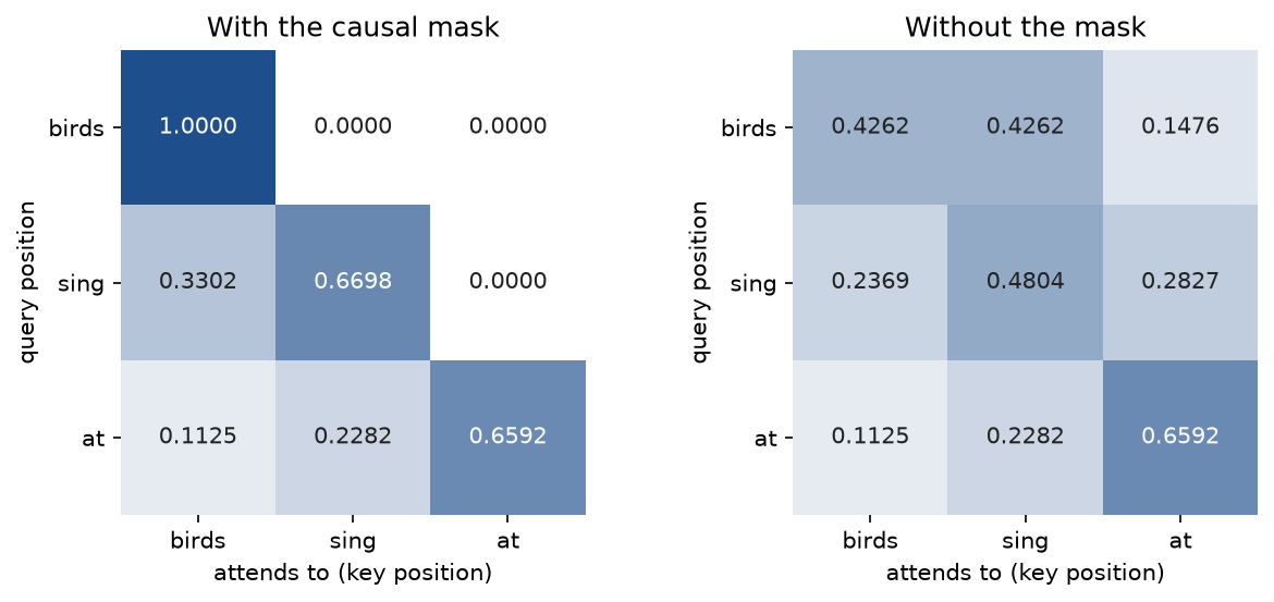
Attention weights of the worked example as two grids, query positions down and key positions across: with the causal mask everything above the diagonal is 0 and row 2 is 0.3302 and 0.6698; without the mask the first row spreads 0.4262, 0.4262 and 0.1476 over all three positions

The left grid is step 5. The right grid shows what the mask prevents, and it leads to two checks on the mask. Replace the third input word "at" by "dawn": the third rows of H and the logits change, to (0.5934, 0.1910) and (0.5934, 0.1910, -0.4979, 0.1057), and the first two rows stay exactly as they were. Remove the mask instead: position 1's weights become (0.4262, 0.4262, 0.1476), so 43 % of its attention goes to position 2, which holds "sing", the very token position 1 is supposed to predict. Every number in this section is asserted by tests/test_trace.py, tests/test_tokenizer.py, tests/test_windows.py and tests/test_encodings.py, and printed by examples/worked_forward_pass.py and examples/tokens_and_windows.py.

The code¶

The package tiny_gpt has a NumPy reference for every piece of the model and a PyTorch mirror written with the same tensor operations, so autograd can train it and the two can be compared number for number. PyTorch and tiktoken are imported only inside the functions that need them.

arrays.py holds the array types, including Parameters, the plain dictionary of named arrays the model lives in.
tokenizer.py holds byte-pair encoding from scratch: train_byte_pair_encoding learns merges and returns ranks and Merge records, byte_pair_merge applies ranks to one chunk lowest rank first, encode_with_ranks, decode_with_ranks and segment work on whole texts, and GPT2_SPLIT_PATTERN is GPT-2's chunking pattern (it needs the regex package, which tiktoken installs).
encodings.py loads tiktoken's encodings into the topic's data folder, turns an encoding's merges into ranks for our own merge loop, and holds the eight-language sentences with token_counts.
datasets.py downloads the book, removes the Project Gutenberg header and licence, joins wrapped lines and checks a pinned digest.
vocabulary.py holds CompactVocabulary, which renumbers the GPT-2 ids a corpus actually uses, and windows.py holds sliding_windows, window_count and split_tokens.
corpus.py puts these together: prepare_corpus and load_book_corpus produce training and validation windows from a contiguous split, and encode_prompt and decode_compact translate between text and compact ids.
config.py holds GPTConfig, GPT-2 small tied and untied, and book_model, the configuration trained below; parameters.py holds parameter_shapes, count_parameters (the closed form), parameter_groups and GPT-2's initialization scheme.
attention.py, layers.py and model.py are the NumPy model: softmax, the causal mask, scaled dot-product and multi-head attention; linear maps, layer norm, both forms of GELU and the MLP; and transformer_block and gpt_logits. losses.py holds cross_entropy and the prediction of the first loss.
trace.py holds worked_example, which builds the micro model, trace_attention_only_model, which keeps every value of its forward pass, and format_attention_trace, which prints them.
sampling.py holds temperature, top-k, choose_next_token and generate, which takes any function from a context to next-token logits.
torch_model.py is the PyTorch mirror, with torch_block, torch_logits, torch_loss, our torch_attention, the library's fused attention and an unmasked variant; training.py holds train_gpt with TrainingSettings, the learning-rate schedule and evaluate_loss.
checkpoints.py saves the parameters, the configuration and the compact vocabulary to one file and loads them back with weights_only=True.
comparisons.py builds the same architecture from torch.nn layers for counting, and measures our functions and attention against PyTorch's; pitfalls.py holds the broken variants of the Pitfalls section; plotting.py draws every figure in the handbook's four colours.

The parameters live in a dictionary keyed by names such as blocks.0.attention.qkv.weight, and a tied model simply has no head.weight: the output layer reads token_embedding. One block of the PyTorch mirror, from torch_block, is the pre-norm equations line by line:

hidden = torch_norm(x, params, prefix + "attention_norm")
qkv = torch_linear(hidden, params, prefix + "attention.qkv")
queries, keys, values = (
    part.reshape(batch, length, heads, d // heads).transpose(1, 2) for part in qkv.split(d, dim=-1)
)
mixed = mix(queries, keys, values).transpose(1, 2).reshape(batch, length, d)
x = x + torch_linear(mixed, params, prefix + "attention.output")
hidden = torch_norm(x, params, prefix + "mlp_norm")
expanded = torch_gelu(torch_linear(hidden, params, prefix + "mlp.expand"))
return x + torch_linear(expanded, params, prefix + "mlp.contract")

mix is torch_attention unless another attention function is passed in, which is how PyTorch's fused attention or a model without a mask is swapped in. The attention itself:

scores = queries @ keys.transpose(-1, -2) / math.sqrt(queries.shape[-1])
future = torch.triu(torch.ones(length, length, dtype=torch.bool, device=queries.device), diagonal=1)
return scores.masked_fill(future, float("-inf")).softmax(dim=-1) @ values

The examples and the project import the package, so install the repository first as described in the main README. Each example demonstrates one idea and runs in a few seconds from the repository root:

examples/worked_forward_pass.py prints every value of the worked example in the order above, the two checks on the mask and the result of masking after the softmax, and saves the attention-weight grids.
examples/tokens_and_windows.py learns the four toy merges, reproduces tiktoken's GPT-2 ids with our merge loop, counts tokens in eight languages under three tokenizers, decodes Korean tokens one by one, and cuts the training pairs of the worked example.
examples/parameter_budget.py counts GPT-2 small three ways, tied and untied, shows that state_dict() counts a tied matrix twice, and compares where the parameters go.
examples/initial_loss.py measures the first loss of GPT-2 small against ln V + s²/2, and the first loss of a small model whose weights are drawn too large.
examples/leaks.py trains a correct model, one without a mask and one with unshifted targets on random tokens, measures the leak of splitting after windowing, and shows PyTorch's two mask conventions.
examples/compare_with_pytorch.py compares the NumPy model with its PyTorch mirror, our functions with PyTorch's, and our attention with scaled_dot_product_attention in agreement and speed.

python transformers-and-llms/tiny-gpt/examples/worked_forward_pass.py
python transformers-and-llms/tiny-gpt/examples/tokens_and_windows.py
python transformers-and-llms/tiny-gpt/examples/parameter_budget.py
python transformers-and-llms/tiny-gpt/examples/initial_loss.py
python transformers-and-llms/tiny-gpt/examples/leaks.py
python transformers-and-llms/tiny-gpt/examples/compare_with_pytorch.py

The sample project, project/train_and_sample.py, trains a small GPT on a real book and writes with it. It downloads The Adventures of Sherlock Holmes, checks the cleaned text against a pinned SHA-256 digest, tokenizes it with GPT-2's encoding and keeps the 8,981 distinct ids the book uses, splits the 145,997 tokens 90 to 10 and cuts windows of 128 tokens: 1,026 for training and 114 for validation. It trains a model of width 128 with 4 heads, 4 layers and a tied output layer, 1,959,296 parameters, for 200 steps of 16 windows with the schedule above, peak learning rate 3 × 10⁻³ and 20 warm-up steps, printing the validation loss every 25 steps. It then saves a checkpoint, loads it back and evaluates it again to prove the file holds the trained model, saves the training curves, and samples from the prompt "Holmes looked at".

The project's pipeline in two rows: the book text, downloaded once and checked; GPT-2 byte-pair encoding; the compact vocabulary of the ids in use; a contiguous split into 90 % training and 10 % validation; windows of 128 tokens with targets shifted by one; AdamW with warm-up, cosine decay and clipping; the checkpoint file in .data/tiny-gpt; and text sampled from a prompt

The pipeline reads left to right along the top row and back along the bottom row. The checkpoint goes to .data/tiny-gpt/tiny-gpt-sherlock.pt at the repository root by default, a folder that is never committed, and --checkpoint writes it anywhere else. Options such as --steps, --width, --heads, --layers, --untied, --learning-rate and --seed change the run, --figures sends the training curves to another folder so a custom run does not overwrite the one shown here, and --sample-only skips training and samples from an existing checkpoint with --prompt, --temperature and --top-k. The default run takes about a minute and a half on one thread and uses about 1 GB of memory.

python transformers-and-llms/tiny-gpt/project/train_and_sample.py
python transformers-and-llms/tiny-gpt/project/train_and_sample.py --sample-only --prompt "Watson said"
python transformers-and-llms/tiny-gpt/project/train_and_sample.py --untied --checkpoint .data/tiny-gpt/untied.pt --figures .data/tiny-gpt

At initialization the validation loss is 9.0960 against ln 8981 = 9.1029. After training it is 5.0733, a perplexity of about 160: the model is about as uncertain as if it chose uniformly among 160 tokens instead of 8,981. The training loss over the last 25 steps averages 4.6219; the gap and the flattening validation curve show the model beginning to memorize a corpus this small.

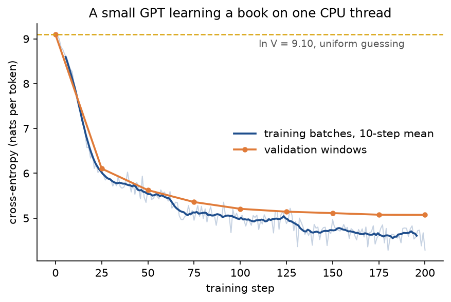
Training and validation loss of the small model on the book over 200 steps: both fall steeply from 9.1, at the dashed amber line of uniform guessing, to about 5.6 by step 50; the validation loss then flattens towards 5.07 while the ten-step mean of the training batches keeps falling to about 4.6

The faint blue line is the loss of each training batch, the dark blue line its ten-step mean and the orange points the validation loss. The curves separate after about 75 steps, a little more than one pass over the training windows.

The same prompt before and after training, with the samples copied from the notebook, which trains the same model with the same seeds as the project. Untrained, at temperature 1, the output is a uniform draw from the book's vocabulary:

Holmes looked at beamiful appir sob dashedpur persist broader complimentary rubbingO spared St admireude authoritativerowing solid uncleastennFrank patience notably resistancezac ushered ImagineVery crushed Christmas Man exceeded removing reference Pennsylvania vileoscope Another

Trained, greedy decoding, with the last token left out because it holds only the first bytes of a closing quotation mark:

Holmes looked at the little-night.
“I have been a little.”

“I have been a little.”

“I have been a little.”
“I have been a little.

Trained, temperature 0.8 with top-k 40:

Holmes looked at the way, a young eyes to me. One were, but a small-handed. I had a man is it was to leave what was not only that the matter. I had got him.”


“There. It

The trained model has learned spelling, punctuation, the layout of dialogue, common phrases and the rhythm of the narration, and nothing about meaning; greedy decoding loops at once. After the prompt, the most probable next tokens at τ = 1 are " the" (0.3370), " his" (0.0876) and " a" (0.0806); at τ = 0.5, " the" alone has 0.8687.

The notebook tiny_gpt.ipynb is a guided tour in the order of this page: the worked example, BPE from scratch and against tiktoken, token counts across languages, the training pairs, the general model with its causality check and its agreement with the PyTorch mirror, the parameter counts and the loss at initialization for GPT-2 small, the pitfalls, the training run, sampling and the comparison with PyTorch's attention. It runs top to bottom in about two minutes on one thread, most of that the training run. The tests in tests check the worked example value by value, the properties above and the agreement with tiktoken and PyTorch, and run in a few seconds:

python -m pytest transformers-and-llms/tiny-gpt

Data: The Adventures of Sherlock Holmes by Arthur Conan Doyle (1892), Project Gutenberg eBook 1661, downloaded on first use into .data/tiny-gpt/ at the repository root. The text is in the public domain in the United States and in every country where copyright ends 70 years or less after the author's death; Doyle died in 1930. Readers elsewhere should check the copyright law of their country, as the Project Gutenberg terms advise. The header and licence are removed before use and nothing is committed. The tokenizer files tiktoken downloads, which it checks against pinned hashes, go to .data/tiny-gpt/tiktoken/. All other examples use synthetic data.

In practice¶

The pieces of the model agree with their library counterparts, measured in examples/compare_with_pytorch.py, the notebook and the tests:

encode_with_ranks with GPT-2's ranks and chunking pattern gives the same ids as tiktoken.get_encoding("gpt2").encode on mixed English, Uzbek, Russian, Korean and Chinese text (tests/test_encodings.py).
torch_attention and torch.nn.functional.scaled_dot_product_attention(q, k, v, is_causal=True) differ by at most 7.2 × 10⁻⁷ in float32 and 1.6 × 10⁻¹⁵ in float64 on the shapes of the training run.
layer_norm, gelu, gelu_exact and cross_entropy agree with F.layer_norm, F.gelu(approximate="tanh"), F.gelu and F.cross_entropy to within 2 × 10⁻¹⁴ relative in float64.
gpt_logits in NumPy and torch_logits in PyTorch agree to within 6 × 10⁻¹⁶ in float64 on the same weights, tied and untied, with our attention or the library's.
count_parameters equals the parameter count of torch.nn layers on the meta device for GPT-2 small, tied and untied.

Swapping the library's attention into a model is one argument:

import torch

from tiny_gpt import GPTConfig, initialize_torch_parameters, library_attention, torch_logits

config = GPTConfig(vocabulary_size=100, context_length=16, width=32, heads=4, layers=2)
params = initialize_torch_parameters(config, seed=0)
ids = torch.randint(0, 100, (2, 16), generator=torch.Generator().manual_seed(0))
ours = torch_logits(params, config, ids)
fused = torch_logits(params, config, ids, attention=library_attention)
print((ours - fused).abs().max().item())

scaled_dot_product_attention never stores the n by n weight matrix when a fused kernel is available, which is what makes long contexts affordable. On the shapes of the training run, on one thread, the library call took 1.7 ms against 3.0 ms for ours in the notebook's run, and swapping it into the trained model leaves the validation loss unchanged to six decimals.

When to use which:

Use the NumPy model to understand and test: every intermediate value can be printed and checked, as in the worked example.
Use the PyTorch mirror, or an equivalent nn.Module such as minGPT or nanoGPT, to train; the functional form here keeps the parameters in a plain dictionary so tying and counting stay visible.
Use scaled_dot_product_attention in anything that has to be fast or handle long contexts, after checking it against a plain implementation as above.
Use tiktoken, or the tokenizer that ships with a pretrained model, rather than a tokenizer of your own. A model is tied to the tokenizer it was trained with.
To work with real GPT-2 weights, load them through Hugging Face Transformers (GPT2LMHeadModel, in the nlp group); this topic describes the same architecture but does not test against that library. Fine-tuning and LoRA starts from such a model.

Pitfalls¶

No causal mask. Without the mask, position t can attend to position t + 1 and read the token it is asked to predict. Training looks wonderful and generation fails, because at generation time the next token does not exist yet. On uniformly random tokens, where nothing can be predicted and the best possible validation loss is ln 64 = 4.1589, an unmasked model reaches 0.5568 within 150 steps while the correct model ends at 4.3374, above ln 64 (examples/leaks.py). Test causality directly: change a token and assert that no earlier logit moves (tests/test_model.py).

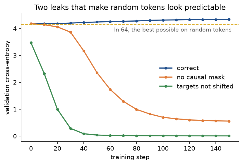
Validation loss on random tokens over 150 steps for three models: the correct model stays just above the dashed amber line at ln 64, the model without a causal mask falls to about 0.56, and the model with unshifted targets falls to almost 0

The correct model can only memorize its training windows, so its validation loss rises slightly above the best possible value; both broken models score far below what is possible on random data, which is the signature of a leak.

Targets not shifted. If the targets are the inputs themselves rather than the inputs moved one token to the right, the model learns to copy its input and the loss collapses; in the same experiment it reaches 0.0065. An off-by-one in the window has the same effect. Assert that the targets without their last column equal the inputs without their first (tests/test_windows.py).
Masking after the softmax. Zeroing the future weights after the softmax leaves rows that no longer sum to one. In the worked example, row 2 becomes (0.2369, 0.4804, 0) with sum 0.7173 instead of (0.3302, 0.6698, 0). Add minus infinity to the scores before the softmax (tests/test_pitfalls.py).
Opposite mask conventions in one library. torch.nn.functional.scaled_dot_product_attention reads a boolean attn_mask as True for "may attend", while torch.nn.MultiheadAttention reads True as "blocked". Handing the matrix of future positions to the first function lets every position see only the future, and the last position, with nothing left to see, outputs zeros (examples/leaks.py). Prefer is_causal=True, and test against a plain implementation.
Not checking the first loss. The loss before any update should be about ln V, or ln V + s²/2 with s = 0.02√d. For V = 2000 and d = 64 the first loss is 7.62 at the usual scale against ln 2000 = 7.6009; with every weight matrix drawn five times too large it is 7.96, twenty-five times 14.37 and fifty times 26.89 (examples/initial_loss.py). Once the logits are large, the loss grows roughly in proportion to s rather than with s². A wrong vocabulary size or misaligned targets show up here too, before any training time is spent.
Counting a tied matrix twice, or tying by arithmetic. state_dict() lists a tied matrix under both of its names, so summing it reports 163,037,184 parameters for the tied GPT-2 small; parameters() yields the shared tensor once and gives 124,439,808 (tests/test_comparisons.py). The opposite mistake is to build a model with a separate output layer and report its size with that layer subtracted: the number on paper matches a tied model, but the model in memory has 163 million parameters and trains two matrices. Tie by making the output layer use the embedding tensor itself.
Showing samples from a model that has not been trained. In a notebook, a generation cell that ran before the training cell, or a training cell interrupted after a few steps, prints text that says nothing about the trained model. Untrained output is a uniform draw from the vocabulary, as in the first sample above. Label every sample with the state of the model that produced it, and run notebooks top to bottom before reading their outputs.
Splitting after windowing. With a stride smaller than the context, every token lies in several windows. Shuffling the windows and then splitting them put 100.0 % of the validation targets into some training window in an example with context 128 and stride 32; splitting the token stream first gives 0.0 %. Split first, then cut windows inside each part (examples/leaks.py).
Decoding one token at a time. A byte-level token can hold part of a UTF-8 character, so decoding tokens one by one prints replacement characters for Korean, Chinese, Hindi and curly quotes; the first nine tokens of the Korean sentence each decode to the replacement character, and the nine together decode to its first word. Decode whole sequences, and expect a sample cut after a fixed number of tokens to end in half a character (tests/test_encodings.py).
Comparing token counts on different text. Tokens depend on case and on the leading space: " Holmes" is one GPT-2 token, " holmes" two and "Holmes" at the start of a text two. Counting tokens on lower-cased text and training on the original gives the wrong number of tokens per pass and the wrong context coverage. Measure on exactly the text the model sees (tests/test_encodings.py).
Feeding more than T tokens. The position table has T rows; position T + 1 does not exist. gpt_logits and torch_logits raise an error and generate crops the context to the last T tokens (tests/test_sampling.py).
Saving a model without its vocabulary, or loading it unsafely. The book model predicts compact ids, which mean nothing without the table that maps them back to GPT-2 ids, so save_checkpoint stores the compact vocabulary next to the parameters and the configuration. load_checkpoint reads the file with weights_only=True, which refuses to run code stored in a checkpoint; that is also why the file holds only tensors, plain numbers and strings, and why a NumPy number left in the metadata would make loading fail (tests/test_checkpoints.py).
Reading the training loss as the model's quality. After 3.1 passes over a small book the training loss averages 4.62 while the validation loss is 5.07 and has almost stopped falling. Judge the model on held-out text, cut from a separate part of the stream.