Backpropagation

Gradient descent trains a network by moving every parameter against the derivative of the cost, so each step needs the derivative of one number with respect to every parameter, and a modern network has millions of parameters. Estimating each derivative separately would take one or two extra forward passes per parameter. Backpropagation gets all of them from a single backward sweep that costs a small constant multiple of the forward pass. This page derives the four equations behind it from the chain rule, runs one mini-batch step through a small network by hand with every intermediate value shown, implements the method in NumPy, and checks the result against finite differences and against PyTorch's automatic differentiation. Afterwards you will be able to compute every gradient of a fully connected network on paper, write a backward pass yourself and verify any gradient code you meet. It builds on Perceptrons and multilayer networks.

To run the code in this topic, install the base group, and the deep group for the comparison with PyTorch.

Intuition

Suppose you could nudge the net input of one unit by a tiny amount and watch the cost. The cost would change by an amount proportional to the nudge, and the factor of proportionality says how much that unit is to blame for the cost. Call this factor the unit's error, δ. Two facts make it the right quantity to track:

• Once a unit's error is known, the gradients of its incoming parameters follow at once. The gradient of a weight is the error at its receiving end times the activation at its sending end, and the gradient of a bias is the error itself.
• A unit's error is fixed by the errors of the units it feeds. Its blame is their blame, sent back along the same weights and scaled by how sensitive the unit's activation is to its net input.

So the method is: run the network forward and remember every intermediate value, compute the error at the output where the cost is directly visible, pass the error backward one layer at a time, and read off the gradients on the way. Each layer reuses the work already done for the layer above it, which is why the whole sweep is cheap.

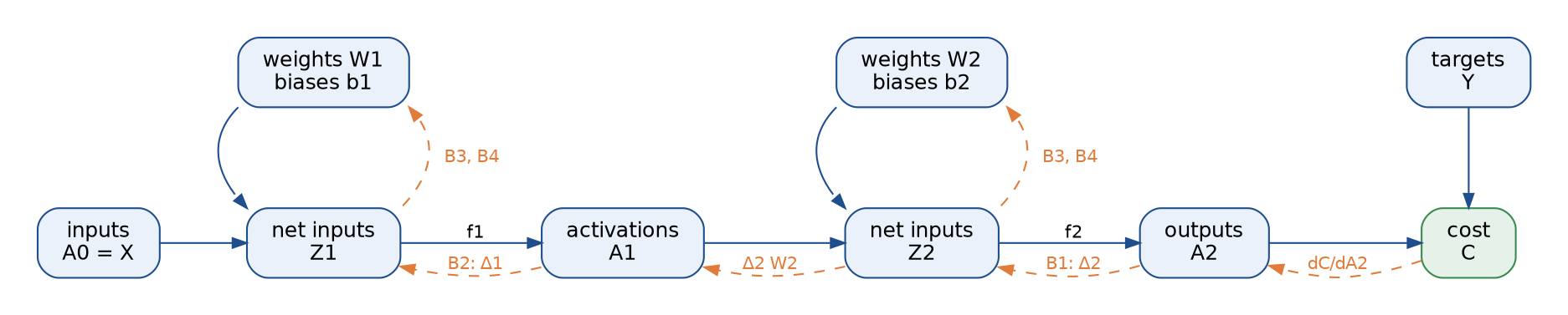
The diagram shows a two-layer network as a computation graph for a whole mini-batch. Solid blue arrows are the forward pass and dashed orange arrows the backward pass; Δ1 and Δ2 hold the errors of layers 1 and 2, one row per example, and B1 to B4 are the four equations derived below.

The second diagram zooms in on one hidden unit. Its error collects the errors of the three units it feeds, each weighted by the connecting weight, and is scaled by the derivative of its own activation. The weight w that brings it its input then receives the gradient δ times a, and the bias receives δ. Everything below is these two sentences made precise.

How it works

Notation and the index convention

The network has L layers of weights. Layer 0 is the input, layer l has n units for l from 1 to L, and layer L is the output. Vectors are columns. For each layer l:

• The weight matrix W has one row per unit of layer l and one column per unit of layer l - 1. Its entry in row j and column k is the weight to unit j from unit k.
• The bias vector b has one entry per unit of layer l.
• The activation function f acts on each entry separately.
• The net inputs z, also called pre-activations, and the activations a hold one value per unit. The activations of layer 0 are the input x.
• The cost C of one example depends on the output activations and the target y.
• The error δ, defined below, holds one value per unit.
• The symbol ⊙ multiplies two vectors entry by entry (the Hadamard product).

The formula images write the layer as a superscript in parentheses. In the text, W1, b1, Z1, A1 and Δ1 are short for the weights, biases, net inputs, activations and errors of layer 1, and likewise for layer 2.

The index convention matters more than any other detail on this page: the first index of a weight is the receiving unit and the second the sending unit, "to j from k". The net input of unit j in layer l is then a sum over the units k of the layer below:

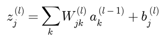
Row j of W holds every weight entering unit j, so a whole layer is one matrix-vector product followed by the activation function:

This is also the layout of torch.nn.Linear.weight, whose shape is (outputs, inputs). Some texts use the opposite order, with the first index the sending unit. Their weight matrices are the transposes of ours and every formula below transposes with them; neither is wrong, but mixing the two is. A gradient always has the shape of the parameter it belongs to, which is a cheap check.

Costs and activations

Until the section on mini-batches, C is the cost of a single example. Writing a for the output activations, two costs appear here: the squared error for any output, and the cross-entropy for outputs in (0, 1) with targets in [0, 1]. Each is shown with its derivative with respect to one output, which is where the backward pass starts.

The factor one half in the squared error is there so that its derivative is simply the difference between output and target.

The derivative of the cross-entropy has a denominator a(1 - a), which will cancel against the sigmoid derivative in a moment.

The activation functions used here are the sigmoid σ, tanh, ReLU and the identity. Their derivatives are best written in terms of the activation a = f(z) wherever possible, because the forward pass has already computed it:

The identity has derivative 1 everywhere. The ReLU derivative does not exist at exactly z = 0, and implementations, ours and PyTorch's included, use 0 there. The sigmoid derivative follows from the chain rule applied to the power -1 and one rearrangement:

The last step uses the fact that the second factor of the product equals 1 - σ(z), since the two fractions add up to one.

The error of a unit

The error of unit j in layer l is the derivative of the cost with respect to its net input:

The derivative is taken at z rather than at a because parameters enter a layer only through z, linearly, and leave it only through f, one entry at a time. With the error defined at z, the bias and weight gradients become one-line consequences.

Every proof below applies the chain rule once, in this form: if C depends on a variable u only through intermediate variables v1 to vn, then

The only skill involved is choosing the intermediate variables correctly: all the variables through which u reaches the cost, and nothing else.

The output error, equation B1

The net input of output unit j reaches the cost only through the outputs, so the chain rule sums over all of them. Because f acts on each entry separately, output k depends on net input j only when k = j, and the sum collapses to a single term:

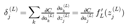
Collecting these for every output unit gives the first equation:

For the squared error, B1 reads (a - y) ⊙ f'(z). For the cross-entropy with a sigmoid output, the derivative of the cost is multiplied by σ'(z) = a(1 - a) and the denominators cancel:

The cancellation is the reason the two are paired: the output error no longer shrinks when a sigmoid output saturates. Loss functions explores the consequences. The collapse of the sum needs an output activation that acts entry by entry. Softmax does not: each of its outputs depends on every net input, the matrix of their derivatives is full, and the output error becomes the transpose of that matrix times the gradient of the cost. For softmax with its matching cross-entropy this again simplifies to a - y.

Passing the error back, equation B2

Unit j of layer l feeds every unit of layer l + 1 and nothing else, so its net input reaches the cost only through the net inputs of layer l + 1. The derivative of each of those with respect to the net input of unit j is the connecting weight times f'(z) of unit j, because the net input of unit i in layer l + 1 is a sum over the activations of layer l and only the term from unit j contains its net input:

The sum runs over the first index of the weight matrix of layer l + 1, the receiving units, so it is entry j of the transposed matrix times the error vector. Collecting over j gives the second equation:

The transpose is not a convention. It appears because the error travels against the direction of the weights: unit j collects blame from every unit it feeds, each share weighted by the connecting weight.

The gradients of the parameters, equations B3 and B4

A bias enters only the net input of its own unit, with derivative 1, so the chain rule leaves a single term:

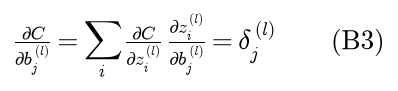
The gradient of a bias is the error of its unit, nothing more. A weight to unit j from unit k appears only in the net input of unit j, multiplied by the activation of unit k, so its derivative is that activation:

The matrix with these entries is the outer product of the error vector with the activations of the layer below, of the same shape as W. B4 says a weight learns in proportion to the error at its receiving end and the activity at its sending end. A weight leaving a unit whose activation is close to zero hardly moves, which is one way saturated sigmoid units and inactive ReLU units slow training down. Together, the four equations read:

B1 starts the backward pass at the output, B2 carries it down one layer at a time, and B3 and B4 turn each layer's errors into the gradients of its parameters.

Mini-batches and the training step

Data usually arrive as a matrix with one example per row, the layout of NumPy, scikit-learn and PyTorch, and the equations are written for that layout here. For a mini-batch of m examples, X holds the inputs and Y the targets. Row i of the matrices Z, A and Δ of a layer holds z, a and δ for example i, where δ is the error of that example's own cost. The cost of the batch is the average of the per-example costs. Let the bold 1 in the formulas be a column of m ones, so that it times the transposed bias adds the bias to every row, and let G have row i equal to the gradient of example i's cost with respect to its outputs; for the squared error, G is simply the output matrix minus Y. Transposing each single-example equation gives one row of a matrix equation:

The forward pass is the layer equation applied to all rows at once. The backward pass and the gradients become:

Two steps deserve a word:

• In the row layout, B2 for one example is a row vector times W rather than the transpose of W times a column vector. That is why the weight matrix appears without a transpose.
• The batch cost is an average, so by linearity of the derivative its gradient is the average of the per-example gradients. The sum over examples of the outer products in B4 is exactly the transposed error matrix times the activation matrix, since entry (j, k) of both is the sum over i of the error of unit j in example i times the activation of unit k in example i. The bias gradient is the column mean of the error matrix.

If examples are stored as columns instead, every matrix above is transposed and the numbers are identical. A gradient descent step with learning rate η > 0 then moves every parameter against its gradient:

One training step on a mini-batch is therefore:

1. Forward pass. Set A0 = X, and for every layer compute and keep Z and A.
2. Output error. Compute the output errors with B1.
3. Backward pass. From the last hidden layer down to layer 1, compute each layer's errors from the layer above with B2.
4. Gradients. For every layer compute the bias gradient with B3 and the weight gradient with B4, both averaged over the batch.
5. Update. Only after every gradient is known, update all weights and biases.

Step 3 must use the weights the forward pass used, and step 2 needs the values the forward pass produced with the current parameters. The procedure therefore starts with a forward pass, not at the output layer, and no parameter changes until step 5. Per layer, the forward pass costs one matrix product and the backward pass two, one for B2 and one for B4. A whole training step therefore costs about three forward passes, however many parameters there are. A finite-difference estimate of the same gradient needs two forward passes per parameter: for a network with a million parameters, two million forward passes instead of about three.

Computation graphs and automatic differentiation

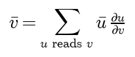
Any computation built from primitive operations forms a directed acyclic graph whose nodes hold values and whose edges show which values each operation reads. For every node v define its adjoint, written with a bar, as the derivative of the cost with respect to v. The chain rule, with the intermediate variables taken to be the nodes that read v, becomes

Reverse-mode automatic differentiation evaluates the graph forward and stores every value, then visits the nodes in reverse order and computes each adjoint from the adjoints of the nodes that read it. Each primitive only has to know how to turn the adjoint of its output into adjoints of its inputs. Each line below is a forward operation, then the arrow, then what its backward step computes:

Chaining these rules through the graph in the first diagram reproduces the four equations. The error δ is the adjoint of z. B1 is the activation rule applied to the adjoint the cost hands back; B2 is the matrix-product rule, which gives the adjoint of the activations as the transposed weights times the adjoint of the next net inputs, followed by the activation rule; B3 is the bias rule; and B4 is the weight half of the matrix-product rule. Backpropagation is reverse-mode automatic differentiation applied to a chain of layers. For a single sigmoid unit the whole procedure fits in two lines, the forward pass above and the backward pass below:

The backward line reads the forward line from right to left, applying one primitive rule at a time.

Forward-mode differentiation pushes derivatives from the inputs towards the output instead and needs one pass for every variable it differentiates with respect to. Reverse mode needs one pass for every output. Training has one output, the cost, and very many parameters, so reverse mode wins by a factor of the parameter count. The price is memory: every value of the forward pass must be stored until the backward pass consumes it, which is why activations, not parameters, often limit the batch size during training. PyTorch's autograd builds the graph on the fly as tensor operations run and performs the backward sweep when backward() is called on the cost; JAX and TensorFlow do the same with traced graphs.

Checking a gradient numerically

Any gradient code can be tested against finite differences, which need nothing but the cost. Nudge one parameter θ by a small step ε and watch the cost. The first line below is the central difference, whose error shrinks like ε squared; the second is the forward difference, whose error shrinks only like ε:

Repeating this for every parameter gives a numerical gradient ĝ to compare with the backpropagated gradient g. Compare them with the relative error, never the absolute difference, which means nothing without the scale of the gradient:

In double precision a relative error below 10⁻⁷ is a pass and one above 10⁻⁴ is almost always a bug.

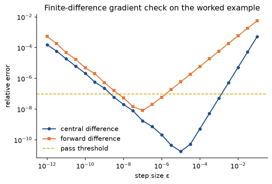
The plot shows both schemes on the worked example below. To the right of each minimum the truncation error of the formula dominates; to the left, rounding error in the difference of two nearly equal costs, roughly 10⁻¹⁶ divided by ε, takes over. Central differences at ε around 10⁻⁵ are the sweet spot in double precision.

Worked example

The network has two inputs, three sigmoid hidden units and one sigmoid output. It is trained with the squared-error cost and learning rate η = 1 on a batch of m = 3 examples.

The diagram gives every parameter. As matrices, the hidden weights W1 have rows (0.4, -0.8), (1.0, 0.6) and (-0.6, 0.2), one row per hidden unit; the hidden biases b1 are (0.1, -0.3, 0.2); the output weights W2 form the single row (1.5, -1.0, 2.0); and the output bias b2 is -0.5. The three examples, the rows of X, are (1.0, 0.5), (-0.5, 1.0) and (0.0, -1.0), with targets 0, 1 and 0.

Every value below is computed in double precision and rounded to four decimals for display. A hand calculation that rounds each intermediate result to four decimals can differ in the last digit; the two places where that happens are pointed out.

Forward pass

Each hidden net input is a row of W1 times the example, plus the bias. For example 1 and hidden unit 1 that is 0.4 × 1.0 + (-0.8) × 0.5 + 0.1 = 0.1. Applying the sigmoid to every entry gives the hidden activations:

• Example 1: hidden net inputs (0.1, 1.0, -0.3), activations (0.5250, 0.7311, 0.4256).
• Example 2: hidden net inputs (-0.9, -0.2, 0.7), activations (0.2891, 0.4502, 0.6682).
• Example 3: hidden net inputs (0.9, -0.9, 0.0), activations (0.7109, 0.2891, 0.5000).

Since σ(-z) = 1 - σ(z), the activations for 0.9 and -0.9 add up to one, which saves work by hand. The output unit combines the three hidden activations with W2 and b2:

• Example 1: output net input 0.4075, output 0.6005, cost 0.1803.
• Example 2: output net input 0.8198, output 0.6942, cost 0.0468.
• Example 3: output net input 1.2774, output 0.7820, cost 0.3058.

For example 1 the output net input is 1.5 × 0.5250 - 1.0 × 0.7311 + 2.0 × 0.4256 - 0.5, which gives 0.4076 from the rounded terms and 0.4075 at full precision. Each cost is one half of the squared difference between output and target, and the batch cost is their mean, (0.1803 + 0.0468 + 0.3058) / 3 = 0.1776.

Backward pass

B1 with the squared error and σ'(z) = a(1 - a) gives one output error per example: the output minus the target, times the sigmoid derivative at the output.

• Example 1: 0.6005 × 0.2399 = 0.1441.
• Example 2: (0.6942 - 1) × 0.2123 = -0.3058 × 0.2123 = -0.0649.
• Example 3: 0.7820 × 0.1705 = 0.1333.

B2 in the row layout first sends each output error back along the output weights, which multiplies it by (1.5, -1.0, 2.0), and then multiplies entry by entry by the sigmoid derivatives of the hidden units:

• Example 1: sent back (0.2161, -0.1441, 0.2881), hidden derivatives (0.2494, 0.1966, 0.2445), hidden errors (0.0539, -0.0283, 0.0704).
• Example 2: sent back (-0.0974, 0.0649, -0.1298), hidden derivatives (0.2055, 0.2475, 0.2217), hidden errors (-0.0200, 0.0161, -0.0288).
• Example 3: sent back (0.2000, -0.1333, 0.2666), hidden derivatives (0.2055, 0.2055, 0.2500), hidden errors (0.0411, -0.0274, 0.0667).

For example 1 and hidden unit 1, δ = 0.1441 × 1.5 × 0.2494 = 0.0539. Hidden unit 3 has the largest error in every example, mostly because its outgoing weight, 2.0, is the largest.

Gradients and update

B3 and B4 average over the batch: each weight gradient adds up, over the three examples, the error at the receiving end times the activation at the sending end, and divides by three.

• Output layer: the gradient of W2 is (0.0505, 0.0382, 0.0282), and the gradient of b2 is (0.1441 - 0.0649 + 0.1333) / 3 = 0.0708.
• Hidden layer: the gradient of W1 has rows (0.0213, -0.0114), (-0.0121, 0.0098) and (0.0283, -0.0201), and the gradient of b1 is (0.0250, -0.0132, 0.0361).

Written out, the first output weight gradient is (0.1441 × 0.5250 - 0.0649 × 0.2891 + 0.1333 × 0.7109) / 3, which is 0.0506 from the rounded terms and 0.0505 at full precision. The top-left hidden weight gradient is (0.0539 × 1.0 + (-0.0200) × (-0.5) + 0.0411 × 0.0) / 3 = 0.0213. Example 3 contributes nothing to the first column because its first input is zero: B4 at work, no activity at the sending end, no gradient.

With η = 1 every parameter moves by minus its gradient:

• W1 becomes the rows (0.3787, -0.7886), (1.0121, 0.5902) and (-0.6283, 0.2201), and b1 becomes (0.0750, -0.2868, 0.1639).
• W2 becomes (1.4495, -1.0382, 1.9718), and b2 becomes -0.5708.

A new forward pass gives outputs (0.5561, 0.6676, 0.7506) and cost 0.1639, down from 0.1776. The output for example 2 moved away from its target of 1: a gradient step lowers the average cost, not every example's cost, and here the two examples with target 0 outweigh it.

Two cross-checks. A central-difference gradient check on this network gives a relative error of about 2 × 10⁻¹⁰. With the cross-entropy cost instead, the output errors would be the outputs minus the targets, (0.6005, -0.3058, 0.7820), between four and six times larger, because the factor σ'(z) no longer multiplies them. Every number in this section is asserted by tests/test_trace.py and printed by examples/worked_step.py.

The code

The package backpropagation is plain NumPy, split into one module per idea. PyTorch is imported only inside the functions of comparisons.py, so everything else works without it.

• arrays.py holds the Array type and as_matrix, which insists on one example per row.
• activations.py holds sigmoid, tanh, ReLU and the identity with their derivatives, each derivative a function of the net input, collected in ACTIVATIONS.
• losses.py holds the squared error and the cross-entropy, per example and as gradients with respect to the outputs, collected in LOSSES.
• propagation.py is the heart of the topic: forward_pass, output_error for B1 and backward_pass for B2 to B4, as plain functions of the parameters.
• network.py holds the frozen MLP class with forward, backward, gradients, cost, predict and step, every update returning a new network, and initialize_mlp for random weights scaled by the fan-in.
• gradient_check.py holds numerical_gradient, relative_error, gradient_check and the helpers that flatten parameters into one vector, together with the twelve activation and cost combinations the tests use.
• trace.py holds worked_example, which builds the network and batch above, trace_step, which keeps every intermediate value of one step, and format_trace, which prints them.
• datasets.py generates the two-moons data from a seed.
• training.py runs mini-batch gradient descent with a reproducible batch order and measures accuracy.
• pitfalls.py holds deliberately broken code for the Pitfalls section.
• comparisons.py builds the same network in PyTorch, computes its gradients with autograd and trains it with torch.optim.SGD.
• plotting.py draws every figure in the handbook's four colours and saves it reproducibly.

Python counts from zero, so weights[0] is W1, and the same holds for biases, net inputs, errors and gradients. The forward pass's activations are the one exception: they start with the inputs, so activations[l] is the activation of layer l. The backward pass in propagation.py is the mini-batch form of B2 to B4 almost symbol for symbol:

for layer in range(len(weights) - 1, 0, -1):
    derivative = ACTIVATIONS[activations[layer - 1]].derivative
    deltas.append((deltas[-1] @ weights[layer]) * derivative(forward.pre_activations[layer - 1]))
deltas.reverse()
weight_gradients = tuple(d.T @ a / count for d, a in zip(deltas, forward.activations[:-1]))
bias_gradients = tuple(d.sum(axis=0) / count for d in deltas)

The examples and the project import the package, so install the repository first as described in the main README. The examples each demonstrate one idea and run in a few seconds at most from the repository root:

• examples/worked_step.py prints every value of the worked example in the order above, then the cross-entropy output errors and their ratio to the squared-error ones.
• examples/check_gradients.py runs the gradient check on the worked example and on all twelve combinations of activations and costs, sweeps the step size for both finite-difference schemes and saves the plot shown under How it works.
• examples/vanishing_errors.py measures the size of the error in every layer of a deep network for four choices of activation and initial scale, for the Pitfalls section.
• examples/common_mistakes.py demonstrates the wrong sigmoid derivative, the missing batch average, updating during the backward pass and symmetric initialization.
• examples/compare_with_pytorch.py compares our gradients with autograd, shows the factor torch.nn.MSELoss introduces, and trains the same model in both frameworks.

python neural-networks/backpropagation/examples/worked_step.py
python neural-networks/backpropagation/examples/check_gradients.py
python neural-networks/backpropagation/examples/vanishing_errors.py
python neural-networks/backpropagation/examples/common_mistakes.py
python neural-networks/backpropagation/examples/compare_with_pytorch.py

The sample project, project/two_moons_classifier.py, applies everything to a small classification task. It generates 400 training and 400 test points of the two-moons problem, two interleaving half circles that no straight line separates, builds a 2-16-1 network with tanh hidden units, a sigmoid output and the cross-entropy cost, and checks its gradients on eight examples before training, because a wrong backward pass is the most expensive bug to discover late. It then runs 300 epochs of mini-batch gradient descent with batches of 32 and learning rate 0.5, prints the training cost every 50 epochs, reports accuracy and saves two figures. Options such as --seed, --hidden, --activation, --epochs, --batch-size and --learning-rate change the setup, and --figures sends the two PNGs to another folder so a custom run does not overwrite the ones shown here; the default run takes about a second.

python neural-networks/backpropagation/project/two_moons_classifier.py
python neural-networks/backpropagation/project/two_moons_classifier.py --activation sigmoid --learning-rate 2.0

With the defaults the training cost falls from 0.9840 to 0.0545, and the network classifies 98.00 % of the training points and 97.75 % of the test points correctly.

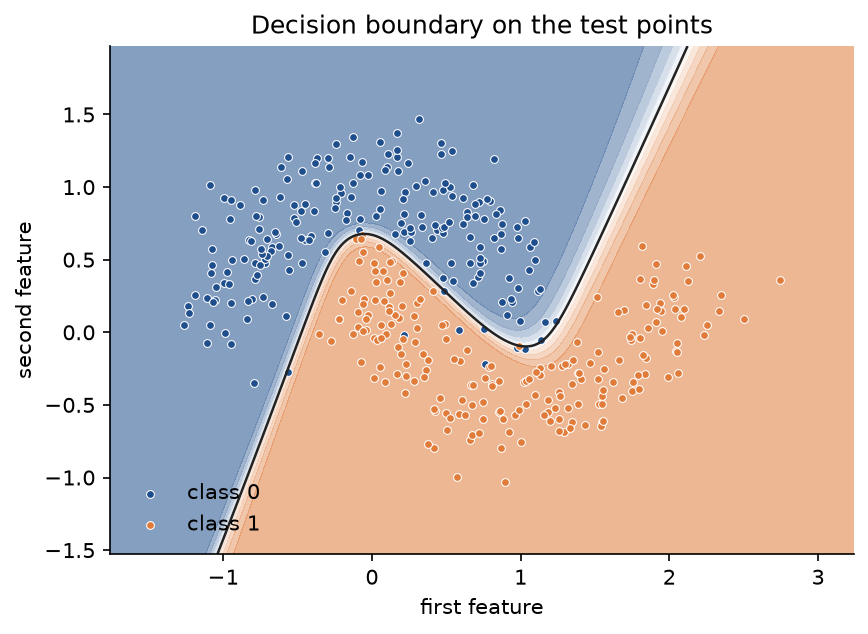
The boundary bends around the tip of each moon, something no single-layer model could draw; the few misclassified points sit where the noise pushes a moon across the gap.

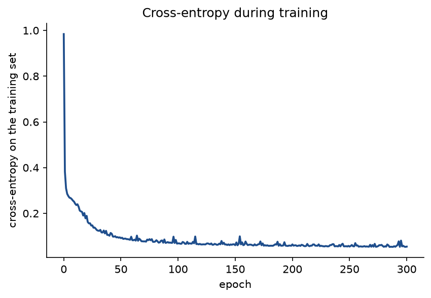
The loss curve drops steeply while the network finds the rough shape of the boundary and then refines it slowly. The small bumps come from mini-batch noise: each step follows the gradient of 32 points, not of the whole training set.

The notebook backpropagation.ipynb is a guided tour in the order of this page: the worked example through trace_step and again in a dozen lines of bare NumPy, gradient checks, each pitfall, training on two moons and the same model in PyTorch. The tests in tests check the worked example value by value, the mathematical properties above and the agreement with PyTorch, and run in a few seconds:

python -m pytest neural-networks/backpropagation

The two-moons data are synthetic, generated by two_moons from a seed, so nothing is downloaded and no licence is involved.

In practice

Production code rarely contains a hand-written backward pass; automatic differentiation derives it. For the same network and the same cost, PyTorch gives the same numbers:

import torch

from backpropagation import to_torch, worked_example

network, inputs, targets = worked_example()
model = to_torch(network)
outputs = model(torch.from_numpy(inputs))
cost = 0.5 * ((outputs - torch.from_numpy(targets)) ** 2).sum(dim=1).mean()
cost.backward()
print(model[0].weight.grad)

In double precision the gradients agree with ours to within about 10⁻¹⁷ on the worked example and 2 × 10⁻¹⁶ across the twelve combinations of hidden activation, output activation and cost. examples/compare_with_pytorch.py then trains the project's network in PyTorch, written the way PyTorch code usually is: torch.nn.Sequential, BCEWithLogitsLoss on the net input of the output unit and torch.optim.SGD. Started from the same weights and fed the same batches, it follows our loss curve to within about 2 × 10⁻¹⁶ and reaches the same 97.75 % test accuracy.

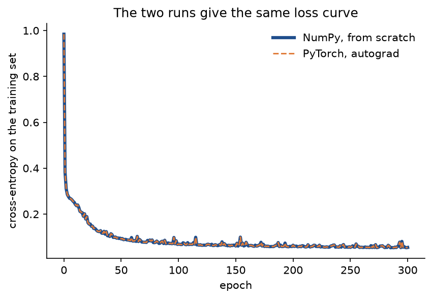
The two curves cannot be told apart, which is the point: the hand-written backward pass and autograd compute the same gradients, so the two runs take the same steps.

When to use which:

• Use the from-scratch version to learn the method, to reason about where gradients vanish or why a layer does not train, and to read papers that write gradients out.
• Use automatic differentiation for anything else. It handles arbitrary graphs, runs on accelerators and is far less error-prone.
• Write a backward pass by hand only for a custom operation, for example a torch.autograd.Function or a fused kernel, and verify it with torch.autograd.gradcheck, which compares it with central differences in double precision, the test described under How it works.
• For a sigmoid output with cross-entropy, prefer BCEWithLogitsLoss on the net input over Sigmoid followed by BCELoss. It is numerically stable for large net inputs, and its gradient with respect to each example's net input is exactly a - y before averaging.

scikit-learn's MLPClassifier and MLPRegressor train by the same backpropagation with SGD, Adam or L-BFGS updates; they are convenient for small tabular problems but expose no gradients.

Pitfalls

• Transposed index conventions. With the first index of a weight meaning the receiving unit, a layer is W times a plus b and the backward step uses the transpose of W; with the opposite convention every matrix is transposed. Mixing conventions fails loudly for non-square layers and silently for square ones. Test with layers of different widths and assert that every gradient has the shape of its parameter, as tests/test_propagation.py does on a 3-5-4-2 network. The same applies to batches stored as rows versus columns.
• Forgetting to average over the batch. If the cost is a mean but the gradients are sums, every gradient is m times too large, which multiplies the learning rate by the batch size and makes the effective step change whenever the batch size does. A gradient check catches it: if the analytic gradient is m times the numerical one, the relative error is exactly (m - 1) / (m + 1), which is 0.5 for the worked example, as examples/common_mistakes.py prints. Libraries expose the choice as reduction="mean" or "sum"; it must match the cost you think you are minimizing.
• The sigmoid derivative written in terms of the wrong quantity. The derivative is σ(z)(1 - σ(z)) = a(1 - a), a function of the activation a, not of z. At z = 1 the correct value is 0.1966; using z(1 - z) gives 0, and applying the sigmoid twice, σ(a)(1 - σ(a)), gives 0.2194, close enough to pass a casual glance. The same slip turns 1 - a² for tanh into 1 - z². In code, the bug is a derivative function that expects z being handed the cached a. examples/common_mistakes.py prints all three values.
• Symmetric initialization. If every weight starts at the same value, every hidden unit computes the same activation, receives the same error through B2 and gets the same gradient through B4, so the units stay identical forever and a layer of width n behaves like a single unit. All-zero weights are worse: B2 multiplies by a zero weight matrix, so on the first step the hidden layer receives no error at all. Random initial weights break the symmetry; biases may start at zero. In examples/common_mistakes.py a 2-16-1 network started with all weights 0.3 keeps sixteen identical hidden units and stops at 87.75 % training accuracy on two moons, against 98.00 % from a random start.
• Exploding or vanishing products. Unrolling B2 shows that the error reaching layer l is a product of one transposed weight matrix and one activation derivative per layer above it. Since the sigmoid derivative is at most 1/4, a deep sigmoid network with moderate weights shrinks the error by about a factor of four per layer, and early layers barely learn; large weights make the product grow instead. examples/vanishing_errors.py measures the size of the error in every layer of a network with ten hidden layers of 32 units. With sigmoid units it falls by six orders of magnitude between the output and the first layer, a factor of 0.24 per layer; with ReLU units and twice the usual initial scale it grows almost a thousandfold. Activations and initialization treats the remedies.

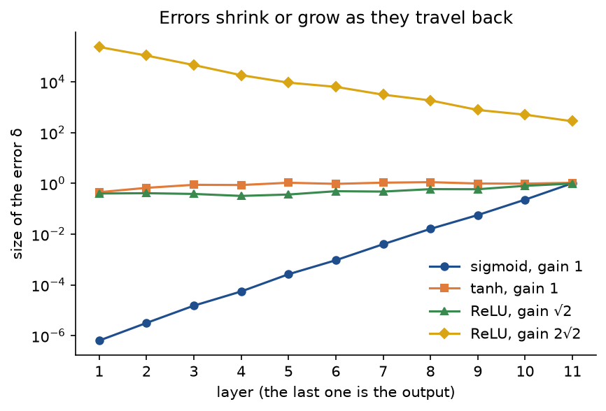
Only the two middle settings keep the error at a usable size in every layer, which is what careful initialization aims for.

• Checking gradients with finite differences incorrectly. Use the central difference, not the forward difference: on the worked example at ε = 10⁻⁵ the central difference has a relative error of 1.8 × 10⁻¹¹ and the forward difference 6.0 × 10⁻⁷, enough to raise a false alarm. Do not make ε tiny either, because rounding error grows as ε shrinks, as the plot under How it works shows. Check in double precision, on a few examples, with dropout and any other randomness switched off, and with any regularization term included on both sides. With ReLU, a net input within ε of zero puts the kink between the two evaluations and gives one large but harmless discrepancy.
• Updating weights during the backward pass. B2 at layer l needs the weights of layer l + 1 as they were during the forward pass. Code that updates each layer as soon as its gradient is known and then propagates the error through the new weights computes the gradient of a network that never existed. The error is small for small learning rates, which makes it easy to miss: on the worked example the hidden-layer gradient is off by a relative 1.2 × 10⁻³ at learning rate 0.1 and 1.3 × 10⁻¹ at 10, while the output layer stays exact. The remedy is to compute every gradient first and update afterwards.
• Comparing against a library loss that is not your cost. torch.nn.MSELoss averages over every entry of the output and has no factor one half, so its gradients are twice ours for one output unit, and in general 2 divided by the number of output units times ours. Agreement tests must spell out the same cost on both sides, as torch_cost does; examples/compare_with_pytorch.py prints the factor.

Further reading

• D. E. Rumelhart, G. E. Hinton and R. J. Williams, "Learning representations by back-propagating errors", Nature 323, 533-536, 1986. The paper that made the method the standard way to train networks.
• S. Linnainmaa, "Taylor expansion of the accumulated rounding error", BIT Numerical Mathematics 16, 146-160, 1976. An early statement of reverse-mode differentiation.
• P. J. Werbos, "Backpropagation through time: what it does and how to do it", Proceedings of the IEEE 78(10), 1550-1560, 1990.
• M. A. Nielsen, Neural Networks and Deep Learning, chapter 2, 2015. A free online book with a careful treatment of the same four equations.
• I. Goodfellow, Y. Bengio and A. Courville, Deep Learning, section 6.5, 2016. Back-propagation on general computation graphs.
• A. G. Baydin, B. A. Pearlmutter, A. A. Radul and J. M. Siskind, "Automatic differentiation in machine learning: a survey", Journal of Machine Learning Research 18(153), 1-43, 2018.
• A. Griewank and A. Walther, Evaluating Derivatives: Principles and Techniques of Algorithmic Differentiation, second edition, SIAM, 2008.
• X. Glorot and Y. Bengio, "Understanding the difficulty of training deep feedforward neural networks", AISTATS 2010. Measures the vanishing errors described under Pitfalls.