Logistic regression

Many prediction problems have a yes-or-no answer: is this tumour malignant, will this customer leave, is this message spam. A useful answer is a probability, not just a label, and the simplest model that produces one is logistic regression: a linear score passed through the sigmoid. Fitting it means maximizing the likelihood of the observed labels, which turns out to be minimizing the cross-entropy, a convex cost whose gradient is just the prediction error times the input. This page explains why ordinary least squares is the wrong tool, derives the cost from the Bernoulli likelihood, derives its gradient and Hessian step by step, proves convexity, and compares gradient descent with Newton's method, which for this model is iteratively reweighted least squares. It covers curved decision boundaries, L1 and L2 regularization, the diverging weights of perfectly separable data, multiclass classification by one-vs-rest and softmax regression, and probability calibration. A worked example runs three gradient descent steps and a full Newton solve by hand, and the implementation is checked against scikit-learn on the breast cancer and digits data. Afterwards you will be able to fit, debug and interpret a logistic regression model, choose its solver and penalty, and tell when its probabilities can be trusted. It builds on Linear regression.

To run the code in this topic, install the base and ml groups.

Intuition

Logistic regression scores an input exactly as linear regression would, with a weight per feature and a bias, and then squashes the score into a probability with the sigmoid σ. A score of 0 means even odds, a large positive score means class 1 is almost certain and a large negative score means class 0 is. The score itself has a meaning: it is the logarithm of the odds p / (1 - p), so each feature adds its weight to the log-odds, and one unit more of a feature multiplies the odds by e raised to its weight.

Training asks which weights make the labels we actually observed most probable. Each example contributes the probability the model gave to its true label: p if the label is 1 and 1 - p if it is 0. Maximizing the product of these, or equivalently minimizing the average of their negative logarithms, gives the cross-entropy cost. A confident mistake costs a lot, because -ln p grows without bound as p approaches 0, while a confident correct prediction costs almost nothing and therefore exerts almost no pull on the weights. That last property is exactly what least squares lacks, and it is why least squares fails for classification.

The gradient of the cost is strikingly simple: for each example, the error p - y times the input. Examples the model already gets right with confidence contribute almost nothing; examples it gets wrong contribute their full input vector, pushing the weights towards them. The cost is convex, so following the gradient cannot get stuck in a bad local minimum, and Newton's method, which also uses the curvature, reaches the minimum in a handful of steps.

The diagram shows the model as a computation for one example: forward along the solid blue arrows, the gradient back along the dashed orange ones. The whole backward pass is two lines long, which is why logistic regression is also the output layer of most classifiers trained with Backpropagation.

How it works

Notation

The data have m examples and n features. The feature matrix X holds one example per row, and the labels y are 0 or 1, with class 1 called positive. For one example with features x:

• The weights w hold one entry per feature, and the bias b is a single number.
• The score z = w · x + b is also called the logit.
• The sigmoid σ(z) = 1 / (1 + e^-z) turns the score into the probability p that the label is 1.
• The parameter vector θ = (b, w) puts the bias first. The augmented matrix, written X with a tilde in the formulas, is X with a column of ones in front, so every score is one entry of the augmented matrix times θ.
• J(θ) is the average cost over the examples, g its gradient with respect to θ and H its Hessian.
• S is the diagonal matrix holding p (1 - p) of every example.
• η is the learning rate of gradient descent, λ the strength of a penalty and K the number of classes.

In the formulas a subscript i counts examples and a subscript j counts features, so p with subscript i is the probability of example i and x with subscripts i and j is feature j of example i. In the text these become "the probability of example i" or, for the worked example, plainly x1, x2, w1 and w2. Logarithms are natural, so costs are in nats.

Everything on this page follows from these two definitions, a linear score and a function that squashes it into a probability, together with the choice of the cost.

Why linear regression is the wrong tool

With labels coded 0 and 1, the quantity we want is the probability that y is 1 given x, and fitting it by least squares is tempting: regress y on x and predict class 1 when the fitted value exceeds one half. This linear probability model has two defects.

1. Its output is not a probability. A linear function of x is unbounded, so for inputs far enough from the data it predicts values below 0 or above 1.
2. Least squares punishes being right with too much confidence. An example with label 1 and fitted value 3 contributes a squared error of 4, so the line tilts to bring it down, even though the example is classified correctly and with a large margin. Points far from the boundary have the most leverage on the fit, exactly the opposite of what classification needs.

examples/why_not_least_squares.py shows the second defect on 60 points with one feature: thirty of class 0 drawn around 2 and thirty of class 1 drawn around 5. On these points the least-squares threshold, at x = 3.2852, and the logistic threshold, at 3.2765, both classify 93.33 % of the points correctly. Adding eight class-1 points far to the right, between 14 and 20, moves the least-squares threshold to 3.9319, and its accuracy on the original points drops to 85 %, while its outputs now range from 0.2734 to 1.3796. The logistic threshold does not move in the first four decimals, because the gradient contribution of a point predicted with probability close to 1 is close to 0.

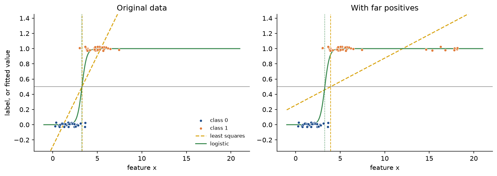
The right panel is the whole argument in one picture: eight points that any classifier gets right drag the least-squares threshold past several points it used to get right. Linear regression is the right tool for a numeric target; for a binary one, the cost has to stop caring about examples that are already right.

The sigmoid and the log-odds

The sigmoid maps the real line onto the interval from 0 to 1, with σ(0) = 1/2, and it is symmetric about that point. Its inverse is the logit, the logarithm of the odds, so logistic regression is the assumption that the log-odds are linear in the features:

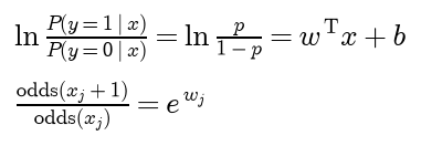
Increasing feature j by one unit adds its weight to the log-odds and multiplies the odds by e raised to that weight, the odds ratio of the feature; with standardized features it is the odds ratio per standard deviation. The effect on the probability itself is not constant. Using the symmetry and the derivative of the sigmoid, derived in Backpropagation:

A feature therefore moves the probability most when p is near one half and hardly at all when the prediction is already confident.

The sigmoid is not an arbitrary choice. Suppose the two classes have prior probabilities π0 and π1 and class-conditional densities f0 and f1. Bayes' rule, from Probability and statistics, gives the posterior as a sigmoid of a log ratio:

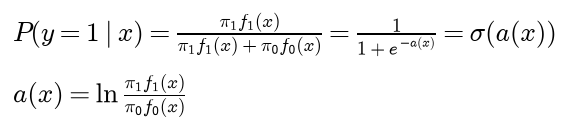
If both densities are Gaussian with means μ0 and μ1 and a shared covariance Σ, the quadratic terms cancel in the log ratio and what remains is linear in x, with

The posterior of this generative model is exactly a logistic regression. Logistic regression fits w and b directly, without modelling how x is distributed, which makes it the discriminative counterpart of generative classifiers such as naive Bayes. When the Gaussian assumption is wrong, as it usually is, fitting the posterior directly is the safer bet.

The Bernoulli likelihood and the cross-entropy cost

The model says that the label, given x, is a Bernoulli variable with success probability p. Both cases fit in one formula, because exactly one of the two exponents is 1:

For independent examples the likelihood is the product over the examples, and its logarithm is a sum:

Maximizing the likelihood is the same as minimizing the average negative log-likelihood, which is the cost used everywhere on this page:

Each per-example term is the cross-entropy between the label's distribution, which puts all its mass on the observed class, and the predicted distribution (p, 1 - p). Information theory explains why that is a natural measure: the cross-entropy is the average code length when data from one distribution are encoded with a code built for another, and it equals the entropy of the first plus the Kullback-Leibler divergence between them. Minimizing the average cross-entropy therefore brings the model's distribution as close as possible, in this sense, to the observed labels. Base-2 logarithms would divide the cost by ln 2 and leave the minimizer unchanged.

Written in terms of the score, the cost loses its awkward logarithms of probabilities. Since ln p = -ln(1 + e^-z) and ln(1 - p) = ln σ(-z) = -ln(1 + e^z):

The simplification uses ln(1 + e^-z) = ln(1 + e^z) - z. This score form is what implementations evaluate, with np.logaddexp(0, z) for ln(1 + e^z), because it never takes the logarithm of a probability that has rounded to 0 or 1. With the labels recoded as t = ±1, the cost is a decreasing function of the margin t z; Support vector machines replace it by the hinge loss max(0, 1 - t z).

The gradient, step by step

Take one example and follow the chain rule from the cost back to a weight. The cost depends on the probability, the probability on the score, and the score on the parameters. Multiplying the three factors, the p (1 - p) of the sigmoid cancels the denominator of the cost:

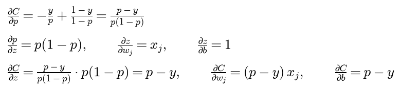
The score form gives the same result in one line: the derivative of ln(1 + e^z) - y z with respect to z is σ(z) - y. Averaging over the examples and stacking the components:

This has the same form as the gradient of the least-squares cost, one over m times the augmented matrix transposed times the residuals, with the probability in place of the linear prediction. The resemblance is not an accident: both are generalized linear models with their canonical link, for which the gradient is always prediction minus target, times input. The algorithms look alike, but the predictions, and therefore the fits, are different.

Setting the gradient to zero shows two properties of every unpenalized fit with an intercept:

The predicted probabilities add up to the number of positives, so their mean equals the observed positive rate, and the same moment matching holds for every feature. The worked example below shows it with five probabilities that add up to exactly 3.

Convexity

Differentiate the gradient once more. The derivative of each probability with respect to a parameter is p (1 - p) times the matching entry of the augmented input, so the Hessian is the augmented matrix weighted row by row:

The labels do not appear: the curvature is the same whatever the labels are. For any direction v the quadratic form is a weighted sum of squares:

So the Hessian is positive semidefinite everywhere and J is convex: every local minimum is a global minimum, and any minimizer found by any method is the minimizer. When the augmented matrix has full column rank, v · x cannot vanish for every example unless v = 0, and since every p lies strictly between 0 and 1 for finite parameters, H is positive definite and J is strictly convex, so there is at most one minimizer. There may be none: the weights p (1 - p) tend to zero as the scores grow, so J is not strongly convex, which is what makes perfect separation possible (below).

The same weights give an upper bound. Since p (1 - p) never exceeds 1/4:

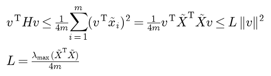
Here λmax is the largest eigenvalue, not a penalty strength. L bounds the curvature of J in every direction, which is what the safe learning rate below needs.

Squared error on a sigmoid output does not share these properties. As a function of the score of a positive example, ½ (σ(z) - 1)² is bounded and not constant, and no such function on the whole real line can be convex. Its plateau for very negative scores is where gradient descent stalls, because its derivative carries the extra factor p (1 - p):

At z = -6 the cross-entropy gradient is -0.9975, while the squared-error gradient is only -0.0025, about four hundred times smaller.

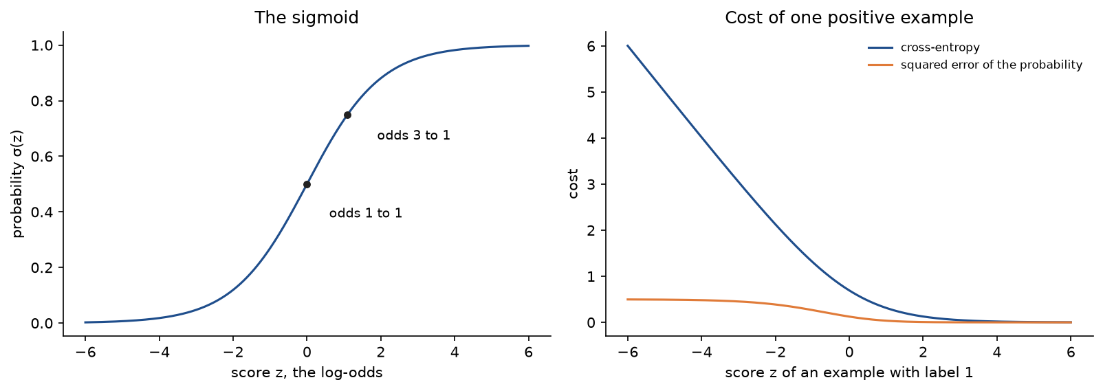
The right panel shows why cross-entropy is the cost to use: it keeps pulling on a confidently wrong example, while squared error has almost given up on it.

Gradient descent

Gradient descent repeats the step below until the gradient is small:

Because the curvature never exceeds L, a standard argument for convex functions shows that every learning rate between 0 and 2 / L lowers the cost at each step and converges to the minimum, when one exists; η = 1 / L is the usual safe choice. Calculus and optimization gives the argument. How fast it converges depends on the condition number of the Hessian, the ratio of its largest to its smallest eigenvalue. Features on very different scales stretch the cost into a narrow valley: the safe learning rate is set by the steepest direction, and progress along the flattest direction crawls. Standardizing the features first, to mean 0 and standard deviation 1 using training statistics only, is therefore part of the method, not a detail.

Stochastic and mini-batch gradient descent replace the average over all m examples by an average over a random batch. The batch gradient is an unbiased estimate of g, each step is much cheaper, and with a learning rate that decreases over time the iterates still converge. This is how logistic regression is trained on data that do not fit in memory, and how it is trained as the last layer of a neural network.

Newton's method and iteratively reweighted least squares

Newton's method uses the curvature as well. Near the current θ the cost is approximately a quadratic in the step d, whose minimum is where its gradient vanishes:

Substituting the Hessian and the gradient from above and multiplying both sides by H turns the step into a familiar problem:

These are the normal equations of a weighted least-squares problem: regress the working response u on the augmented features with weight p (1 - p) on each example. Each Newton step solves one such problem with weights and responses recomputed from the current fit, hence the name iteratively reweighted least squares, or IRLS. Examples whose probability is near one half, the uncertain ones near the boundary, get the most weight. With an L2 penalty (below) the matrix on the left gains m λ on the diagonal entries of the weights, but not of the bias.

The diagram shows one step. irls_step in the package computes it exactly this way, and a test confirms that it equals the Newton step written with the Hessian.

At θ = 0 every probability is one half, every weight is 1/4 and the working response is 4 (y - 1/2), so the first Newton step from zero is ordinary least squares on targets of ±2. Close to the optimum Newton's method converges quadratically: the error is roughly squared at every step, so the number of correct digits doubles. Without a penalty it is also invariant to any invertible affine transformation of the features: shifted and rescaled features give correspondingly transformed iterates and exactly the same predictions, so standardization does not change its path. Far from the optimum a full step can overshoot, and the implementation here halves the step until the cost decreases, a safeguard that is rarely needed for logistic regression.

The two methods trade cost per iteration against the number of iterations:

• Gradient descent uses only the gradient. Each iteration costs one pass over the data, of the order of m n operations, and needs memory for n numbers, but reaching high accuracy takes hundreds to many thousands of iterations, more as the condition number grows. It needs a learning rate, stable below 2 / L, and it needs scaled features.
• Newton's method uses the gradient and the Hessian. Each iteration costs of the order of m n² operations to form the Hessian and n³ to solve the system, and memory for n² numbers, but it typically finishes in 5 to 15 iterations, quadratically near the optimum. It needs no tuning, and without a penalty its iterates do not depend on feature scaling.
• Gradient descent suits very many features, streaming data and mini-batches; Newton's method suits up to a few thousand features with all the data in memory.

Quasi-Newton methods such as L-BFGS, scikit-learn's default solver, sit in between: they build an approximation of the inverse Hessian from the last few gradients and get much of Newton's speed at the cost per iteration of gradient descent.

Decision boundaries

With the rule "predict class 1 when p is at least one half", the boundary is where the score is 0:

The boundary is a hyperplane, a line for two features, with normal vector w. The score of a point divided by the length of w is its signed distance from the boundary, and every contour of constant probability is a parallel hyperplane. Using another threshold shifts the boundary in parallel without refitting; choosing it is a question for Evaluation metrics.

A linear boundary is a statement about the features, not about the method. Replace x by a feature map φ(x) and the boundary is linear in φ but curved in x. Polynomial features of degree d contain every product of at most d original features; for two features and degree 2 they are x1, x2, x1², x1 x2 and x2², and the weights (0, 0, -1, 0, -1) with bias r² give the score r² - x1² - x2², positive exactly inside the circle of radius r. The cost is still convex in θ and everything above still applies, because the model is still linear in its parameters. The number of features grows quickly, and a flexible boundary can wrap itself around noise, which is what regularization is for.

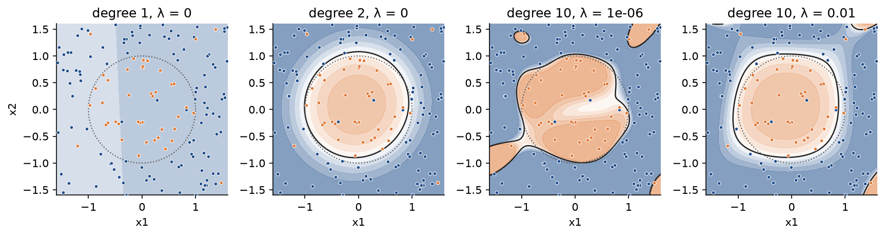
examples/regularization.py fits these four models. A line classifies 65.76 % of 5000 fresh points correctly; degree 2, with five features, reaches 88.60 %, close to the 92 % that the flipped labels allow. Degree 10 has 65 features for 150 points: with λ = 10⁻⁶ it needs 21 Newton steps, its weights have length 185.5 and it scores 98.00 % on the training points but 84.82 % on fresh ones. With λ = 0.01 the weights shrink to length 3.1 and fresh accuracy recovers to 86.82 %. A single logistic unit is also the building block of neural networks, which learn the feature map instead of fixing it.

Regularization

A penalty on the size of the weights is added to the cost. The bias is left out, because shifting all scores by a constant says nothing about the complexity of the boundary:

The L2 penalty, also called ridge or weight decay, adds λ w to the gradient and λ to the diagonal entries of the Hessian that belong to the weights, so a gradient step shrinks the weights and then steps. Every eigenvalue of the weight block of the Hessian is now at least λ, so the penalized cost is strongly convex in w and, as long as both classes occur, has exactly one minimizer, separable data or not. In Bayesian terms the penalized cost is, up to scaling and a constant, the negative log posterior under a Gaussian prior on the weights, so the fit is the posterior mode.

The L1 penalty, also called the lasso, corresponds to a Laplace prior and has a kink at zero, which is what produces exact zeros. At a minimizer the subgradient conditions hold:

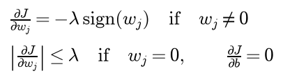
A feature whose gradient at zero is smaller than λ in absolute value stays out of the model entirely. Because the absolute value is not differentiable at 0, plain gradient descent does not apply. Proximal gradient descent takes a gradient step on the smooth part and then applies soft thresholding, the exact minimizer of ½ (v - u)² + t |v|:

The implementation adds Nesterov momentum with adaptive restart, the accelerated method known as FISTA, which needs far fewer iterations on the same problems. The elastic net mixes the two penalties.

Both penalties depend on the scale of each feature: a feature measured in millimetres instead of metres needs a weight a thousand times smaller and is penalized a million times less under L2, so features are standardized before fitting a penalized model. Libraries usually parameterize the strength differently. scikit-learn multiplies the summed, not averaged, per-example costs by a constant C and adds the penalty without a factor:

A larger C means a weaker penalty, and the same C means a different λ when the number of examples changes.

Perfect separation

Suppose some hyperplane separates the classes perfectly, so that its score is positive for every positive example and negative for every negative one. In the margin form of the cost, scaling these parameters by a factor c drives the cost to zero:

Every term tends to zero because every margin t z is positive. Every term is also strictly positive for finite parameters, so the value 0 is approached but never reached: the cost has no minimizer and the maximum-likelihood estimate does not exist. Gradient descent keeps lowering the cost by growing the weights without bound, asymptotically like the logarithm of the number of steps, while the direction of w, and with it the boundary, converges slowly to the maximum-margin direction of a hard-margin support vector machine. Newton's method takes ever larger steps while its Hessian approaches singularity. Since the gradient tends to zero along the way, any stopping rule based on the gradient eventually reports convergence, at weights that are meaningless and probabilities that are all 0 or 1. If only some examples can be separated, which is called quasi-separation, some weights diverge and the others converge.

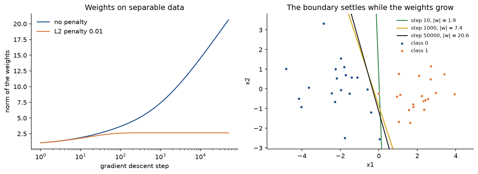
examples/common_mistakes.py runs gradient descent with η = 1 on forty points in two clusters four standard deviations apart. The length of w is 1.8787 after 10 steps, 7.4183 after 1000, 14.5503 after 10,000 and 20.6328 after 50,000, when the cost is 3.37 × 10⁻⁴, while its direction settles near (0.9609, 0.2769). With λ = 0.01 the length stops at 2.6444. Newton's method reports convergence after 24 steps with weights of length 75.9, and scikit-learn without a penalty returns weights of length 22.0 without a single warning.

Separation is common: m ≤ n + 1 points in general position are always linearly separable, and many real data sets with far fewer features than examples are separable too, the breast cancer data used below among them. Any λ > 0 restores a unique, finite solution; early stopping and Firth's bias-reduced likelihood are alternatives. A single feature that separates the classes perfectly deserves suspicion before it is trusted, because it may be a leak (Data leakage and pitfalls).

Multiclass: one-vs-rest and softmax regression

For more than two classes there are two common extensions.

One-vs-rest trains K binary models, model k separating class k from all others, and predicts the class whose model gives the highest probability. Each model is trained independently, so their probabilities do not sum to one; libraries divide by the sum afterwards, which makes them sum to one without making them consistent. Each binary problem is also imbalanced, one class against K - 1.

Softmax regression, also called multinomial logistic regression, models all classes jointly. Class k has its own weight vector and bias, and the probabilities are the softmax of the scores:

The probabilities are positive and sum to one by construction, and the largest score gets the largest probability.

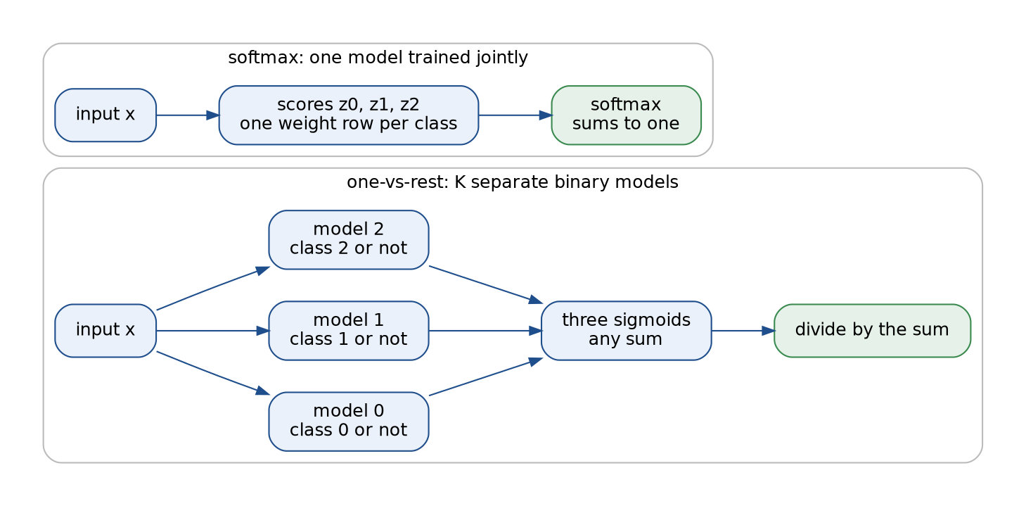
The diagram contrasts the two. With the label one-hot encoded, so that the entry of the true class c is 1 and the others are 0, the categorical likelihood gives the cost

Differentiating the second form with respect to the score of class k, the first term gives -1 for the true class and 0 otherwise, and the log-sum-exp gives exactly the probability of class k. So the gradient is again probability minus target, times input:

Here P and Y are the m by K matrices of probabilities and one-hot labels, and W stacks the weight vectors as rows. The same result follows from the Jacobian of the softmax, as Loss functions shows for a network's output layer. The Hessian block for classes k and l weights the augmented features of every example by p of class k times (1 if k = l, else 0, minus p of class l); the whole Hessian is again positive semidefinite, so the cost is convex.

Two details matter in practice. First, the parameterization is redundant: adding the same vector to every weight vector and the same constant to every bias adds the same amount to every score and leaves every probability unchanged. The cost is flat along those directions and its Hessian singular. An L2 penalty removes the redundancy for the weights, since among all equivalent solutions it prefers the one whose weight vectors sum to zero; the unpenalized biases are fixed by convention, for example by making them sum to zero, which is what scikit-learn reports and what the minimum-norm Newton step in this package keeps. For two classes only the difference matters, and softmax regression reduces to logistic regression with w = w1 - w0 and b = b1 - b0. Second, e^z overflows double precision above about 709, so the softmax is computed after subtracting the largest score from every score, which does not change the result.

Probability calibration

A classifier is calibrated if, among all examples to which it assigns probability q, a fraction q is positive. Logistic regression minimizes the log loss, a strictly proper scoring rule, one whose expected value is minimized only by the true probabilities, so a correctly specified, unpenalized model fitted to enough data is calibrated. In any sample, its intercept condition makes the mean predicted probability on the training data equal the observed positive rate. Several common practices break calibration:

• A strong penalty pulls every score towards zero and every probability towards the middle. The model is underconfident, and its reliability curve is steeper than the diagonal.
• Overfitting, many irrelevant features or near separation make the probabilities too extreme. The model is overconfident, and the curve is flatter than the diagonal.
• Resampling or class weights change the base rate the model learns. Repeating every positive k times multiplies the training odds by k, which adds about ln k to the intercept; subtracting ln k from the fitted intercept restores the original base rate. For a correctly specified model, sampling positives at k times the rate of negatives changes only the population intercept, by exactly ln k; in a finite sample the correction is close but not exact.

Calibration is measured with a reliability diagram, the observed fraction of positives against the mean predicted probability in bins of predictions, and summarized by the expected calibration error (ECE), by the Brier score and by the log loss itself:

examples/calibration.py draws data from a known logistic model with three features, 400 training rows and 20,000 test rows, whose test positive rate is 0.4144. The five fits score as follows, each with ECE, Brier score, log loss and mean predicted probability on the test rows:

• Maximum likelihood: 0.0174, 0.1548, 0.4699 and 0.4318.
• A strong L2 penalty, λ = 0.5: 0.1647, 0.1966, 0.5820 and 0.4257.
• Every positive repeated three times: 0.1850, 0.1954, 0.5786 and 0.5994.
• The same fit with its intercept lowered by ln 3: 0.0164, 0.1540, 0.4677 and 0.4308.
• Sixty pure-noise features added: 0.1141, 0.1973, 0.6207 and 0.4146.

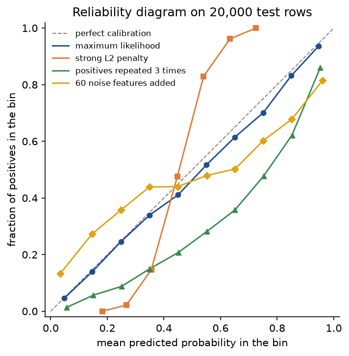
The plain fit is well calibrated. The penalized fit is underconfident and the noisy fit overconfident, both with a mean probability close to the base rate, while the oversampled fit predicts too many positives across the board until its intercept is corrected. Calibration is not discrimination: any increasing transformation of the scores leaves the ranking, and hence the ROC curve, unchanged while changing calibration completely (Evaluation metrics). Platt scaling recalibrates another model's scores by fitting a one-feature logistic regression to them on held-out data.

Worked example

Five examples with two features, written as (x1, x2) with their labels: (1, 3) with label 1, (2, 0) with label 0, (3, 1) with label 1, (3, 2) with label 0 and (4, 1) with label 1. The parameters start at θ = (b, w1, w2) = (0, 0, 0) and the learning rate is η = 0.5.

No line separates the classes: the segment joining the two negatives, from (2, 0) to (3, 2), crosses the triangle formed by the three positives, so the convex hulls of the classes overlap and the minimizer exists. Every value below is computed in double precision and rounded to four decimals for display; a calculation that rounds each intermediate result can differ in the last digit, as noted where it happens.

Three steps of gradient descent

Iteration 1. With θ = 0 every score is 0, every probability is one half and the cost is ln 2 = 0.6931. The residuals p - y are (-0.5, 0.5, -0.5, 0.5, -0.5), and each component of the gradient is the average of the residuals times the matching input, a constant 1 for the bias:

The step θ ← θ - 0.5 g gives θ = (0.05, 0.15, 0.15), and the cost drops to 0.6531.

Iteration 2. Now each score is 0.05 + 0.15 (x1 + x2), and the sums x1 + x2 are 4, 2, 4, 5 and 5:

• Scores: 0.6500, 0.3500, 0.6500, 0.8000 and 0.8000.
• Probabilities: 0.6570, 0.5866, 0.6570, 0.6900 and 0.6900.
• Residuals p - y: -0.3430, 0.5866, -0.3430, 0.6900 and -0.3100.

The bias gradient is (-0.3430 + 0.5866 - 0.3430 + 0.6900 - 0.3100) / 5 = 0.0561. The gradient for w1 weights the residuals by 1, 2, 3, 3 and 4 and gives 0.1262; the gradient for w2 weights them by 3, 0, 1, 2 and 1 and gives -0.0604. The step gives θ = (0.05 - 0.0281, 0.15 - 0.0631, 0.15 + 0.0302) = (0.0219, 0.0869, 0.1802) and the cost 0.6451. The first step overshot the bias: every probability is now above one half although two labels are 0, so the bias gradient changed sign and the bias moves back down.

Iteration 3. With θ = (0.0219, 0.0869, 0.1802):

• Scores: 0.6494, 0.1957, 0.4628, 0.6430 and 0.5497.
• Probabilities: 0.6569, 0.5488, 0.6137, 0.6554 and 0.6341.
• Residuals: -0.3431, 0.5488, -0.3863, 0.6554 and -0.3659.

The gradient is (0.0218, 0.0196, -0.0941), the step gives θ = (0.0111, 0.0771, 0.2273) and the cost falls to 0.6406. The new bias is 0.0219 - 0.0109 = 0.0110 from the rounded terms and 0.0111 at full precision. Over the three steps w2 grows steadily while w1 rises and falls back: the data say that x2 matters more.

The learning rate is safe. The augmented matrix transposed times itself has largest eigenvalue 51.6675, so L = 51.6675 / 20 = 2.5834 and gradient descent is guaranteed to lower the cost for any η below 2 / L = 0.7742. It is also slow: the cost is still 0.0359 above the optimum after 10 steps and 0.0103 after 100, and it takes a little under 900 steps to get within 10⁻⁶.

Newton's method

At θ = 0 every weight p (1 - p) is 1/4, so the first Newton step is least squares on the targets 4 (y - 1/2) = (2, -2, 2, -2, 2). Its normal equations are three linear equations in the bias and the two weights:

The coefficients are the sums of the ones, the features and their products over the five examples, and the right-hand sides are the sums of the targets times the same columns. The determinant is 111 and the solution is exactly θ = (-230, 56, 92) / 111 = (-2.0721, 0.5045, 0.8288), with cost 0.5930: one step gets most of the way. Repeating the step with the weights and working responses recomputed each time:

• Iterate 0: θ = (0, 0, 0), cost 0.6931, gradient norm 4.359 × 10⁻¹.
• Iterate 1: θ = (-2.0721, 0.5045, 0.8288), cost 0.5930, gradient norm 2.693 × 10⁻².
• Iterate 2: θ = (-2.2957, 0.5534, 0.9156), cost 0.5923, gradient norm 4.262 × 10⁻⁴.
• Iterate 3: θ = (-2.3025, 0.5548, 0.9180), cost 0.5923, gradient norm 2.351 × 10⁻⁷.
• Iterate 4: the same parameters to four decimals, gradient norm about 3 × 10⁻¹³.

The gradient norm roughly squares at each step, the signature of quadratic convergence: four Newton steps reach rounding level, against hundreds of gradient descent steps for six digits.

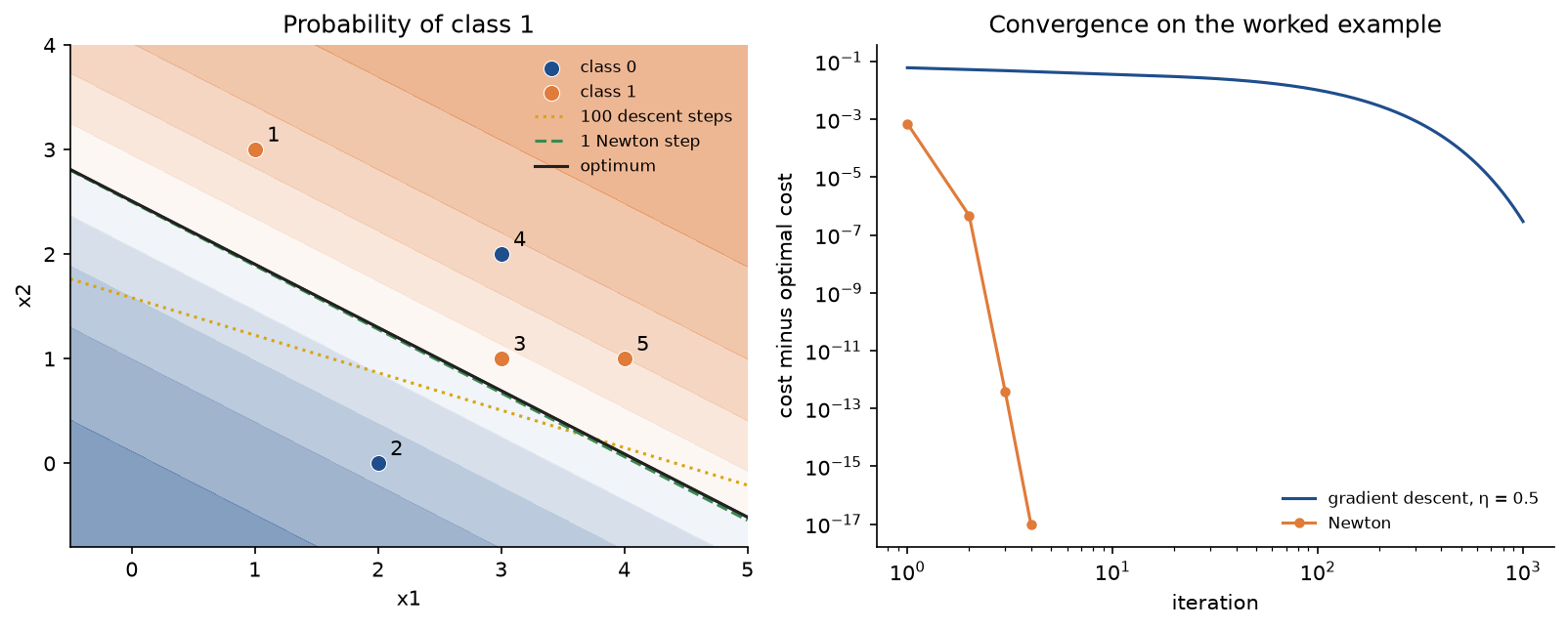
The left panel shows how close one Newton step already is to the optimal boundary, while 100 gradient descent steps still tilt it visibly. Example 4, the blue point on the orange side, is the one the optimum misclassifies.

Reading the optimum

The minimizer is θ = (-2.3025, 0.5548, 0.9180), with cost 0.5923. The fitted probabilities are 0.7323, 0.2327, 0.5695, 0.7681 and 0.6973; they add up to exactly 3, the number of positives, as the intercept condition requires. Example 4 is misclassified with probability 0.7681 for a label 0, the price of a linear boundary on data that are not linearly separable.

• The odds ratios are e^0.5548 = 1.7415 and e^0.9180 = 2.5043: one unit more of x1 multiplies the odds of class 1 by 1.74, one unit more of x2 by 2.50.
• A new point (2, 2) has score -2.3025 + 0.5548 × 2 + 0.9180 × 2 = 0.6431 and probability σ(0.6431) = 0.6554.
• The decision boundary is 0.5548 x1 + 0.9180 x2 = 2.3025, or x2 = 2.5081 - 0.6043 x1.

scikit-learn's LogisticRegression without a penalty returns the same parameters to within 10⁻⁶.

One softmax step

Three classes, one example x = (1, 2) of class 0, and a softmax model whose weight rows are (0.5, -0.2), (0.1, 0.4) and (-0.3, 0.1), with biases 0.2, -0.1 and 0.0.

• The scores are 0.5 - 0.4 + 0.2 = 0.3, 0.1 + 0.8 - 0.1 = 0.8 and -0.3 + 0.2 + 0.0 = -0.1.
• Their exponentials are 1.3499, 2.2255 and 0.9048, which sum to 4.4802, so the probabilities are 0.3013, 0.4967 and 0.2020, and the cost is -ln 0.3013 = 1.1997.
• The gradient with respect to the scores is p - y = (-0.6987, 0.4967, 0.2020). It is also the bias gradient, and the weight gradient is its outer product with the input: the rows (-0.6987, -1.3974), (0.4967, 0.9935) and (0.2020, 0.4039).

The second column is twice the first. Doubled from the rounded first column it would read -1.3974, 0.9934 and 0.4040; at full precision the last two are 0.9935 and 0.4039. A step with η = 0.1 changes the score of class k by -η (p - y) (1 + |x|²) = -0.6 (p - y), because each score depends only on its own weight row and its own bias. The new scores are 0.7192, 0.5020 and -0.2212, the probabilities 0.4555, 0.3666 and 0.1779, and the cost 0.7863: the true class gained probability at the expense of both others, most from the class that had the most. Every number in this section is asserted by tests/test_trace.py and tests/test_newton.py and printed by examples/worked_steps.py.

The code

The package logistic_regression is plain NumPy, split into one module per idea. scikit-learn is imported only inside the data loaders and comparisons.py, so everything else works without it.

• arrays.py holds the Array type, as_matrix, which insists on one example per row, as_binary_labels and with_intercept.
• sigmoid.py holds sigmoid, log_sigmoid and logit, all numerically stable.
• model.py holds the frozen LogisticModel with decision_function, predict_proba, predict and the conversions to and from θ = (b, w), and FitResult, which every optimizer returns with the path of iterates, the costs, the gradient norms and a convergence flag.
• cost.py is the heart of the topic: cross_entropy evaluated from the scores with optional L2 and L1 terms, gradient, parameter_gradient, hessian and smoothness_constant for L.
• descent.py holds gradient_descent, and newton.py holds newton, built on the damped loop damped_newton and newton_direction, and irls_step, the same step written as weighted least squares.
• regularization.py holds soft_threshold, proximal_gradient for L1, accelerated with adaptive restart, and regularization_path, which fits both penalties over a range of strengths.
• softmax.py holds softmax, log_softmax, one_hot and SoftmaxModel with its cost, gradient and Hessian; multiclass.py fits it by fit_softmax_gradient_descent or fit_softmax_newton, and holds OneVsRestModel with fit_one_vs_rest.
• features.py holds polynomial_features in scikit-learn's column order, the Standardizer and a PolynomialClassifier that chains them with a fit.
• metrics.py holds accuracy, log_loss, multiclass_log_loss, brier_score and confusion_counts; calibration.py holds calibration_curve, expected_calibration_error and calibration_study, the experiment above.
• gradient_check.py compares the analytic gradient and Hessian with central differences.
• trace.py holds worked_example, softmax_worked_example and trace_gradient_descent, which keeps every intermediate value of each step, with format_trace to print them.
• datasets.py holds the synthetic generators, the loaders of the two bundled data sets and standardized_split, which splits by class and standardizes with training statistics.
• pitfalls.py holds deliberately fragile code for the Pitfalls section, comparisons.py builds the equivalent scikit-learn models, and plotting.py draws every figure in the handbook's four colours.

The gradient and the Hessian are a few lines each. Without the input checks, cost.py computes them as

residuals = model.predict_proba(features) - labels
weight_gradient = features.T @ residuals / features.shape[0] + l2 * model.weights
bias_gradient = float(np.mean(residuals))

curvature = probabilities * (1.0 - probabilities)
matrix = augmented.T @ (augmented * curvature[:, None]) / features.shape[0]
matrix[1:, 1:] += l2 * np.eye(features.shape[1])

and the IRLS form of the Newton step in newton.py is

weights = probabilities * (1.0 - probabilities)
working_response = augmented @ model.parameters + (labels - probabilities) / weights
normal_matrix = augmented.T @ (augmented * weights[:, None]) + penalty
parameters = np.linalg.solve(normal_matrix, augmented.T @ (weights * working_response))

The examples and the project import the package, so install the repository first as described in the main README. The examples each demonstrate one idea and run in a few seconds from the repository root:

• examples/worked_steps.py prints every value of the worked example in the order above: the three gradient descent steps, the Newton iterates, the reading of the optimum and the softmax step.
• examples/why_not_least_squares.py compares least squares with logistic regression on one feature and the two costs of a confident mistake.
• examples/newton_vs_gradient_descent.py finds the learning rates gradient descent survives on the worked example and races the two methods on the breast cancer data with standardized and with raw features.
• examples/regularization.py fits polynomial boundaries to the ring, traces the L2 and L1 paths on the breast cancer data and checks the L1 fit against scikit-learn's saga solver.
• examples/calibration.py runs the calibration experiment and draws its reliability diagram.
• examples/common_mistakes.py demonstrates perfect separation, a cost computed from rounded probabilities, a gradient missing its 1 / m, swapped class coding, a softmax without the shift and the penalized intercept of liblinear.

python machine-learning/logistic-regression/examples/worked_steps.py
python machine-learning/logistic-regression/examples/why_not_least_squares.py
python machine-learning/logistic-regression/examples/newton_vs_gradient_descent.py
python machine-learning/logistic-regression/examples/regularization.py
python machine-learning/logistic-regression/examples/calibration.py
python machine-learning/logistic-regression/examples/common_mistakes.py

The sample project, project/tumour_classifier.py, applies everything to two real tasks.

The first task is the Breast Cancer Wisconsin (Diagnostic) data: 569 tumours described by 30 features computed from digitized images of fine-needle aspirates, such as the radius, texture and concavity of the nuclei, each as a mean, a standard error and a worst value, with 212 malignant tumours. A stratified split keeps 171 rows for testing, and the standardization uses training statistics only. With λ = 1/m, scikit-learn's default, Newton's method converges in 9 steps, the gradient norm falling from 1.4 to 8.8 × 10⁻¹³. On the test rows the model classifies 165 of 171 tumours correctly, an accuracy of 0.9649: it finds 60 of the 64 malignant tumours and calls 2 of the 107 benign ones malignant. The test log loss is 0.1169, the Brier score 0.0283 and the expected calibration error 0.0259. The largest coefficients are worst texture (+1.3618, an odds ratio of 3.9031 per standard deviation), mean concavity (+1.1503) and worst radius (+1.0012). With strongly correlated features such as the radius, perimeter and area of the same nucleus, individual coefficients are not reliable measures of importance, even though the predictions are.

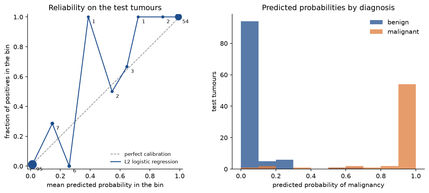
Most tumours get a probability below 0.1 or above 0.9, and those two bins, holding 95 and 54 tumours, are where calibration can actually be judged; the middle bins hold one to seven tumours each and their scatter is sampling noise. The second task is the optical handwritten digits data: 1,797 images of 8 by 8 pixels, ten classes, with 539 images kept for testing. Softmax regression with λ = 1/m has 650 parameters and converges in 9 Newton steps; it classifies 96.47 % of the test images correctly with a test log loss of 0.1181. One-vs-rest with the same penalty reaches 96.10 % and a log loss of 0.1695: the jointly trained model gives better probabilities.

Each weight vector, drawn as an image, shows which pixels raise or lower the score of its class; the zero, for example, is penalized for ink in the centre, where a zero has its hole. The project finally fits scikit-learn's models on the same data and prints how far apart the two implementations are, the numbers quoted under In practice. Options such as --seed, --test-fraction, --strength, --bins, --skip-digits and --skip-sklearn change the setup, and --figures sends the PNGs to another folder so a custom run does not overwrite the ones shown here; the default run takes about two seconds.

python machine-learning/logistic-regression/project/tumour_classifier.py
python machine-learning/logistic-regression/project/tumour_classifier.py --strength 0.05 --skip-digits

The notebook logistic_regression.ipynb is a guided tour in the order of this page: least squares against logistic regression, the worked example through trace_gradient_descent and again in bare NumPy, Newton's method and the softmax step, gradient and Hessian checks, curved boundaries, calibration, each pitfall, and the breast cancer and digits runs with the comparison against scikit-learn. The tests in tests check the worked example value by value, the mathematical properties above and the agreement with scikit-learn, and run in a few seconds:

python -m pytest machine-learning/logistic-regression

Data: the breast cancer and digits data ship with scikit-learn, so nothing is downloaded. The Breast Cancer Wisconsin (Diagnostic) data were created by W. H. Wolberg, W. N. Street and O. L. Mangasarian (1995), and the Optical Recognition of Handwritten Digits data by E. Alpaydin and C. Kaynak (1998); both are distributed by the UCI Machine Learning Repository under the Creative Commons Attribution 4.0 licence. The breast cancer target is recoded so that malignant is 1. Every other data set is synthetic and generated from a fixed seed.

In practice

The library equivalent is sklearn.linear_model.LogisticRegression. Its default is an L2 penalty with C = 1, that is λ = 1/m. On recent versions the penalty is chosen with l1_ratio, 0 for L2 and 1 for L1, and a model without a penalty needs C equal to infinity; older versions take penalty instead, which sklearn_logistic handles. For the breast cancer model above:

from sklearn.linear_model import LogisticRegression

from logistic_regression import load_breast_cancer_data, newton, standardized_split

features, labels, names = load_breast_cancer_data()
split = standardized_split(features, labels, test_fraction=0.3, seed=0)
m = len(split.train_y)
ours = newton(split.train_x, split.train_y, l2=1.0 / m).model
theirs = LogisticRegression(C=1.0, tol=1e-12, max_iter=10_000).fit(split.train_x, split.train_y)
print(abs(theirs.coef_.ravel() - ours.weights).max())

With the conversion C = 1/(λ m) and tight tolerances the two agree, as the project and the tests show:

• Breast cancer with L2 and λ = 1/m: scikit-learn's lbfgs needs 37 iterations, and the coefficients differ by at most 9.4 × 10⁻⁷, the intercepts by 3.3 × 10⁻⁷ and the test probabilities by 3.7 × 10⁻⁷.
• Breast cancer with L1 and λ = 0.05, against the saga solver: the coefficients differ by 3.8 × 10⁻¹¹, and both keep the same three features, worst radius, worst texture and worst concave points.
• Digits with softmax regression and λ = 1/m, against the multinomial lbfgs fit: test probabilities within 8.7 × 10⁻⁷, coefficients within 1.1 × 10⁻⁶, and the same predictions.
• Digits with one-vs-rest, against OneVsRestClassifier: test probabilities within 1.4 × 10⁻⁶ and the same predictions.

The remaining differences are scikit-learn's stopping tolerance, not disagreement about the solution. On synthetic problems tests/test_comparisons.py asserts the same agreement for the worked example, three L2 strengths, an L1 fit, softmax and one-vs-rest, and tests/test_metrics.py and tests/test_calibration.py check the metrics against sklearn.metrics and sklearn.calibration.

Which solver to choose:

• lbfgs, the default, is a quasi-Newton method; it handles L2 and no penalty, binary and multinomial.
• newton-cholesky is Newton's method as derived above; it is the fastest choice when there are many more examples than features and the features number at most a few hundred.
• liblinear handles L1 and L2 on small data sets but fits multiclass problems one-vs-rest and penalizes the intercept (see Pitfalls).
• saga handles L1 and the elastic net on large data sets; it is stochastic and needs standardized features to converge in reasonable time.
• SGDClassifier(loss="log_loss") trains by stochastic gradient descent for data that do not fit in memory.

In PyTorch the same model is a torch.nn.Linear layer with torch.nn.BCEWithLogitsLoss for two classes or torch.nn.CrossEntropyLoss for K classes, both computing the cost from the scores as derived above; that version is not tested here. For confidence intervals and hypothesis tests on the coefficients, the inverse of the unscaled Hessian at the optimum, the augmented matrix transposed times S times the augmented matrix, is the usual estimate of the covariance of θ, which is what statistical packages report as standard errors.

Gradient descent against Newton's method on real data

examples/newton_vs_gradient_descent.py minimizes the penalized breast cancer cost both ways. With standardized features, gradient descent at the safe learning rate 1 / L is still 1.6 × 10⁻² above the optimum after 100 steps, 4.2 × 10⁻⁴ after 1,000 and 1.8 × 10⁻⁷ after 5,000, while Newton's method reaches rounding level in 9 steps. On the raw features, whose scales range from about 10⁻³ to 10³, the condition number of the Hessian at the optimum grows from 4.0 × 10¹ to 1.7 × 10⁹; gradient descent is still 0.16 above the optimum after 5,000 steps, while Newton's method needs 10.

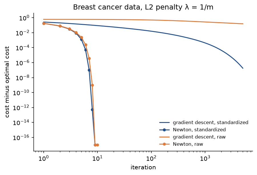
The plot is the condition number made visible: Newton's method does not care how the features are scaled, gradient descent cares a great deal.

Regularization paths

examples/regularization.py fits both penalties at fifteen strengths from 1 down to 3.2 × 10⁻⁴. The L2 coefficients grow smoothly from zero, each fit taking 5 to 11 Newton steps. The L1 path brings features in one after another: none at λ = 1, 3 at λ = 0.1, 8 at λ = 0.01, 13 at λ = 0.001 and 16 at 3.2 × 10⁻⁴. Test accuracy of the L1 fits peaks at 0.9708 with 9 or 10 features, at λ between 3.2 × 10⁻³ and 5.6 × 10⁻³, and falls on either side: too few features underfit, and too many overfit data that are separable without a penalty. The proximal method needs up to almost 9,000 iterations per fit, far more than Newton's method, which the kink of the L1 penalty rules out. Choosing λ by test accuracy, as this list invites, would leak; in practice it is chosen by cross-validation on the training rows (Evaluation metrics).

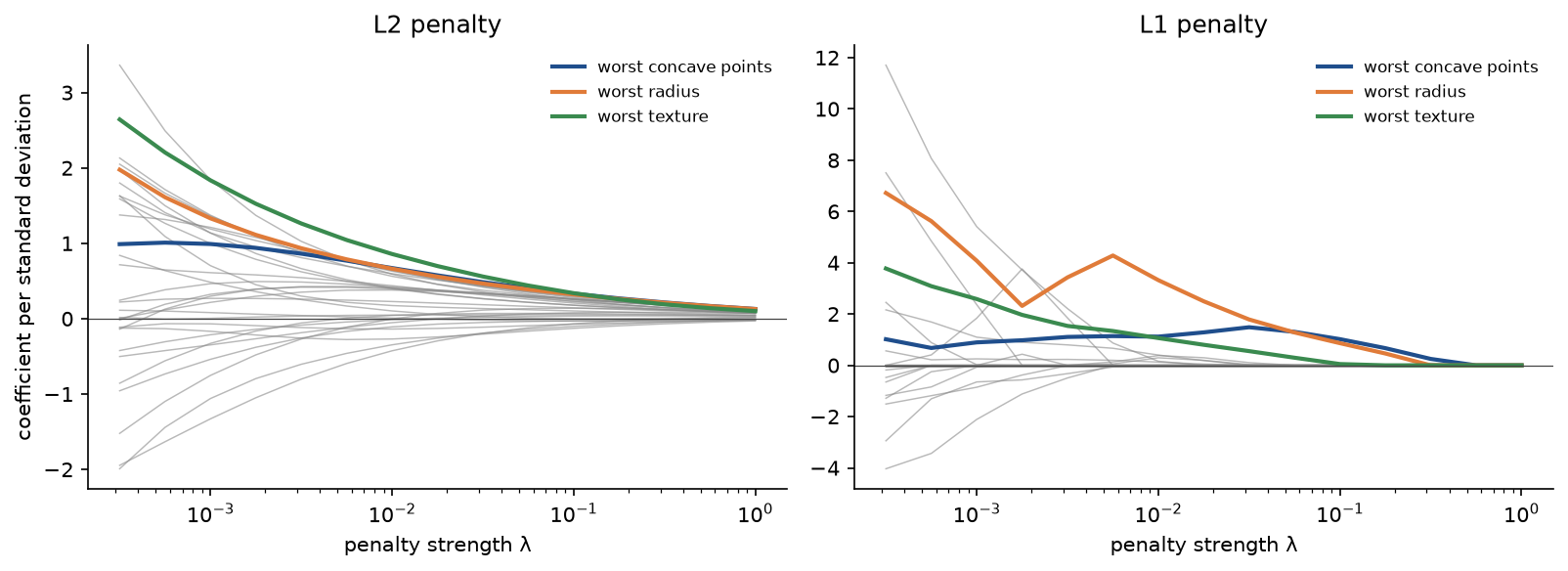
The highlighted features are the three the L1 fit keeps at λ = 0.1, the strongest penalty that keeps three. Under L2 they shrink smoothly along with everything else; under L1 they are the last survivors as the penalty grows. The L1 path also shows correlated features trading places: at λ = 0.32 the second feature in the model is worst perimeter, which gives way to worst radius at 0.18, and below 3.2 × 10⁻³ the coefficient of worst radius dips while that of worst area rises.

When to use which

• Use the from-scratch Newton solver to learn the method and for small problems where you want every intermediate quantity; it is exact to rounding error in a handful of steps.
• Use scikit-learn for real work, with standardized features inside a pipeline, the default L2 penalty as a starting point and C chosen by cross-validation.
• Use logistic regression as the first model on any tabular classification problem. It trains in seconds, its coefficients can be read, its probabilities are usually well calibrated, and a more complex model has to beat it to justify itself. It is also the standard baseline for text classification on bag-of-words features (Text classification).

Pitfalls

• Regressing the 0 and 1 labels by least squares. The fit produces "probabilities" outside the unit interval, and easy, far-away points drag the threshold: eight easy positives move the least-squares threshold from 3.2852 to 3.9319 and cut its accuracy on the original points from 0.9333 to 0.8500, while the logistic threshold stays at 3.2765 (examples/why_not_least_squares.py, tests/test_pitfalls.py).
• Squared error on a sigmoid output. The cost is not convex in the weights, and its gradient vanishes for confident mistakes: at z = -6 it is -0.0025 against -0.9975 for cross-entropy.
• Computing the cost from rounded probabilities. σ(40) rounds to exactly 1 in double precision, so ln(1 - p) is minus infinity for a confident mistake. Evaluate ln(1 + e^z) - y z with logaddexp: in examples/common_mistakes.py the probability form gives inf and the score form 40.0000. Clipping probabilities to a small distance from 0 and 1 hides the problem and changes the gradient.
• Not noticing perfect separation. Without a penalty the weights diverge, and solvers still report success because the gradient vanishes along the way. The 398 standardized training rows of the breast cancer data are separable: unpenalized Newton reports convergence after 25 steps with weights of length 348.4 and training accuracy 1, and 98.25 % of its test probabilities are below 0.001 or above 0.999, giving a test log loss of 1.4182 against 0.1169 with λ = 1/m. Check the length of the weights and the training accuracy, and keep a penalty (examples/common_mistakes.py, tests/test_datasets.py).
• Unscaled features with a gradient method. The condition number of the Hessian on the raw breast cancer features is 1.7 × 10⁹, and 5,000 gradient descent steps leave the cost 0.16 above its minimum. Standardize with statistics from the training rows only, fitting the scaler inside the cross-validation loop (Data leakage and pitfalls).
• A learning rate that is too large. The bound 2 / L guarantees that every step lowers the cost, but it is pessimistic, because it assumes the largest possible curvature. On the worked example 2 / L = 0.7742, and η = 0.8 still converges with the cost falling at every step; η = 0.9 still converges, though the cost rises on 51 of its 3,000 steps. What gradient descent cannot survive is a step above 2 divided by the curvature at the optimum, here 2 / 2.1200 = 0.9434: with η = 0.95 and η = 1.0 the iterates oscillate around the minimum indefinitely, still 0.0046 and 0.0339 above it after 3,000 steps. The cost sequence shows the problem at once (examples/newton_vs_gradient_descent.py, tests/test_descent.py).
• Penalizing the intercept. The penalty is meant for the weights. scikit-learn's liblinear solver treats the intercept as the weight of a constant feature and penalizes it: on 2,000 rows with 9.1 % positives and λ = 0.5, its mean predicted probability is 0.3660 and its intercept -0.5501, while the unpenalized intercept of our fit, -2.3067, keeps the mean probability at exactly 0.0910, as lbfgs does (examples/common_mistakes.py). Written derivations sometimes include the bias in the penalty sum or in weight decay by mistake; the gradient with respect to b should never contain λ.
• Confusing C with λ. scikit-learn's C is an inverse strength attached to the summed, not averaged, cost: C = 1/(λ m). A larger C means less regularization, and the same C on twice the data is half the λ.
• A gradient that does not match its cost. A common slip is to define the cost as an average but drop the 1/m from the gradient, which multiplies the effective learning rate by m. A central-difference check catches it at once: on the worked example the averaged gradient agrees to a relative error of 5.9 × 10⁻¹¹, while the summed one is off by exactly (m - 1)/(m + 1) = 0.6667 (examples/common_mistakes.py, tests/test_gradient_check.py). Another slip is the sign of the update, adding the gradient of the cost instead of subtracting it, which is correct only when ascending the log-likelihood.
• Forgetting which class is coded 1. scikit-learn's copy of the breast cancer data codes malignant as 0. Swapping the coding negates every coefficient and the intercept and turns every p into 1 - p: the two parameter vectors sum to zero within 6.1 × 10⁻¹⁶. A coefficient read as a risk factor then has the wrong sign.
• Trusting probabilities after resampling or class weights. Repeating every positive three times raises the expected calibration error from 0.0174 to 0.1850 and the mean predicted probability from 0.4318 to 0.5994; subtracting ln 3 from the intercept brings the error back to 0.0164 (examples/calibration.py, tests/test_calibration.py). Class weights can be the right choice for a decision; they are not a free fix for imbalance, and the threshold can be moved instead.
• Reading one-vs-rest probabilities before normalization. On the digits test images the ten raw one-vs-rest probabilities of an image sum to anything from 0.0312 to 1.9648 (project/tumour_classifier.py).
• Exponentiating raw scores in the softmax. For scores around 1000, np.exp overflows and the softmax returns nan; subtracting the largest score first gives (0.2447, 0.6652, 0.0900) (examples/common_mistakes.py, tests/test_softmax.py).
• Interpreting coefficients causally or individually. A coefficient is the change in log-odds per unit of its feature with all other features held fixed. With correlated features, such as the radius, perimeter and area of a nucleus, that situation hardly occurs in the data, the coefficients trade off against each other, and L1 keeps one of a correlated group almost arbitrarily. Odds ratios also depend on the feature's unit, so compare them only on standardized features.

Further reading

• D. R. Cox, "The regression analysis of binary sequences", Journal of the Royal Statistical Society B 20(2), 215-242, 1958. The paper that introduced logistic regression for binary outcomes.
• P. McCullagh and J. A. Nelder, Generalized Linear Models, second edition, Chapman and Hall, 1989. Canonical links and iteratively reweighted least squares in general.
• T. Hastie, R. Tibshirani and J. Friedman, The Elements of Statistical Learning, second edition, Springer, 2009, section 4.4. Logistic regression, IRLS and L1-penalized fits.
• C. M. Bishop, Pattern Recognition and Machine Learning, Springer, 2006, sections 4.2 and 4.3. The generative derivation of the sigmoid, IRLS and multiclass logistic regression.
• K. P. Murphy, Probabilistic Machine Learning: An Introduction, MIT Press, 2022, chapter 10. A modern treatment including optimization and Bayesian logistic regression.
• A. Albert and J. A. Anderson, "On the existence of maximum likelihood estimates in logistic regression models", Biometrika 71(1), 1-10, 1984. Separation, quasi-separation and when the estimate exists.
• D. Firth, "Bias reduction of maximum likelihood estimates", Biometrika 80(1), 27-38, 1993. The penalized likelihood that stays finite under separation.
• D. Soudry, E. Hoffer, M. S. Nacson, S. Gunasekar and N. Srebro, "The implicit bias of gradient descent on separable data", Journal of Machine Learning Research 19(70), 1-57, 2018. Why the direction converges to the maximum-margin solution while the length grows logarithmically.
• R. Tibshirani, "Regression shrinkage and selection via the lasso", Journal of the Royal Statistical Society B 58(1), 267-288, 1996.
• A. Beck and M. Teboulle, "A fast iterative shrinkage-thresholding algorithm for linear inverse problems", SIAM Journal on Imaging Sciences 2(1), 183-202, 2009. The accelerated proximal gradient method used for L1.
• B. O'Donoghue and E. Candès, "Adaptive restart for accelerated gradient schemes", Foundations of Computational Mathematics 15, 715-732, 2015.
• G. King and L. Zeng, "Logistic regression in rare events data", Political Analysis 9(2), 137-163, 2001. The intercept correction after sampling on the outcome.
• J. C. Platt, "Probabilistic outputs for support vector machines and comparisons to regularized likelihood methods", in Advances in Large Margin Classifiers, MIT Press, 1999. Platt scaling.
• A. Niculescu-Mizil and R. Caruana, "Predicting good probabilities with supervised learning", Proceedings of the 22nd International Conference on Machine Learning, 2005. An empirical study of calibration across model families.
• W. N. Street, W. H. Wolberg and O. L. Mangasarian, "Nuclear feature extraction for breast tumor diagnosis", Proceedings of SPIE 1905, 861-870, 1993. The source of the breast cancer features.