Linear regression

Linear regression predicts a number as a weighted sum of input features, and least squares picks the weights that make the squared prediction errors as small as possible. It is the first model worth fitting to almost any numeric target, the baseline every flexible model has to beat, and the place where the central ideas of machine learning appear in their simplest exact form: a cost function, its minimum found in closed form or by gradient descent, the effect of feature scaling on the optimizer, feature engineering, regularization and honest measures of fit. This page derives the normal equation twice, by calculus and by projection, analyses gradient descent through the eigenvalues of the cost's curvature so that the price of unscaled features can be predicted in iterations, derives ridge regression in closed form and the lasso's coordinate-descent update with soft-thresholding, and states R-squared and adjusted R-squared correctly. A five-point example is worked by hand, everything is implemented in NumPy, and a sample project models house prices in California with engineered features and penalties chosen on validation data, checked against scikit-learn. Afterwards you will be able to fit and diagnose a linear model by hand and in code, predict how many gradient-descent iterations a problem needs, choose and tune a penalty, and read a residual plot. It builds on Linear algebra for machine learning and Calculus and optimization.

To run the code in this topic, install the base group, and the ml group for the California housing data and the comparisons with scikit-learn.

Intuition

Plot the data as points and look for the straight line that runs closest to them. For each point the vertical gap between the point and the line is a residual: the amount by which the line misses that target. Least squares chooses the line that makes the sum of the squared residuals as small as possible. Squaring stops positive and negative misses from cancelling, punishes one large miss more than several small ones and, most usefully, turns the total error into a smooth bowl over the space of possible lines, with a single lowest point that can be found exactly.

There are two ways to the bottom of the bowl. The first is to solve for the point where the bowl is flat in every direction; that is a system of linear equations, the normal equation, and it gives the answer in one step. The second is to start anywhere and walk downhill, which is gradient descent. Walking is slower for small problems but works when there are too many features to solve the system, when the data arrive in pieces, and for models whose bowl has no closed-form bottom, such as logistic regression and neural networks. How fast the walk goes depends entirely on the shape of the bowl: a round bowl is descended in a few steps, a long narrow valley takes thousands. The shape is set by the units of the features, which is why feature scaling, irrelevant to the exact solution, matters so much to gradient descent.

"Linear" refers to the parameters, not to the inputs. Squares, products, logarithms and indicators of the features can be added as new columns and the model is still fitted by the same least squares. More columns fit the training data better and new data worse, so the weights are often penalized: ridge regression shrinks all of them towards zero, the lasso sets some exactly to zero. Finally the fit is judged by the share of variance it explains on data it has not seen, and by plotting the residuals, which show what a single number hides.

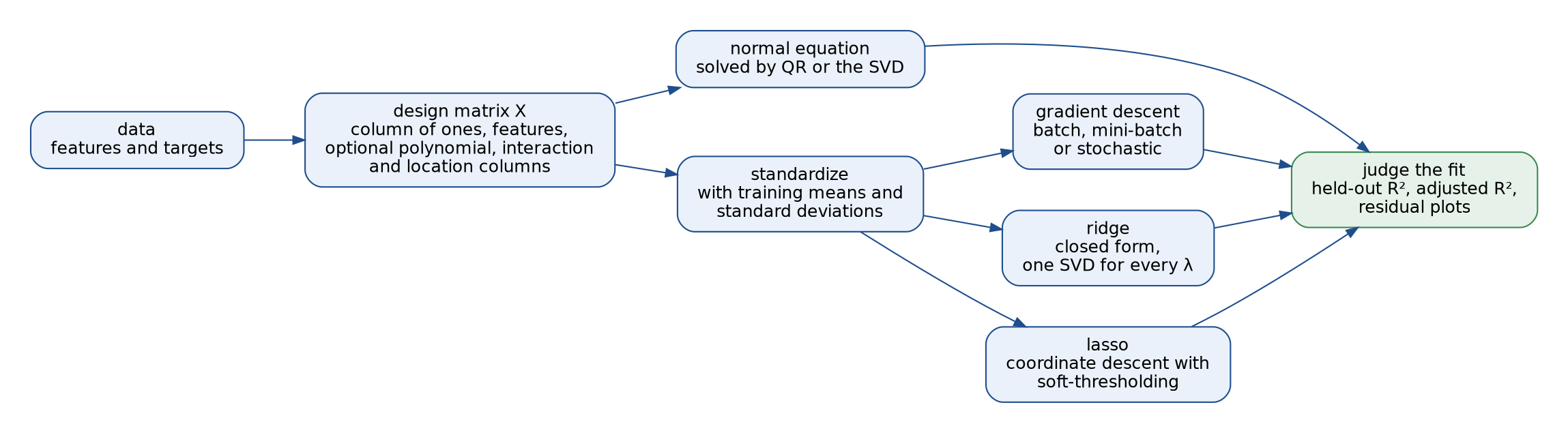
The diagram is the map of this page. The exact route never needs feature scaling; the three routes through standardization do, gradient descent for speed and the two penalties for fairness between features. Every route ends in the same place, because a fit is only as good as the evidence that it works on new data.

How it works

Notation

Vectors are columns. There are m examples and n features.

• The design matrix X has one row per example. Row i starts with a 1, which carries the intercept, and continues with the n features of example i. The formula images write that row as the transposed vector x with superscript (i); the text calls it x(i).
• The targets form the vector y, with mean ȳ; the bold 1 in formulas is the vector of m ones.
• The parameters θ = (θ0, θ1, ..., θn) are the intercept θ0 and the slopes. When the intercept is handled separately, the slopes alone are called w.
• Predictions are ŷ = Xθ and residuals r = y - ŷ. RSS, TSS and ESS are the residual, total and explained sums of squares.
• The cost J(θ) is RSS divided by 2m. Its curvature matrix A = XᵀX / m has eigenvalues λ1 to λ(n+1), the largest λmax and the smallest λmin, and condition number κ = λmax / λmin.
• The learning rate is η and the mini-batch size b.
• Penalty strengths are λ for ridge and α for the lasso. A λ with an index, such as λk, is always an eigenvalue of A.
• Feature j has training mean μj and standard deviation sj. A tilde marks data with their training means subtracted: X̃, ỹ, and x̃j for column j of X̃.

The model and the squared-error cost

The model predicts a weighted sum of the features plus an intercept, one example at a time or for all examples at once:

The column of ones carries the intercept, so it needs no special treatment. The residual sum of squares and the cost are:

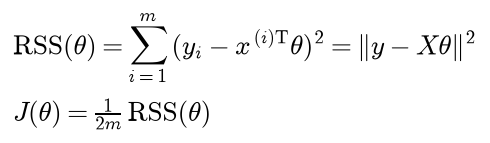
The factor 1/m makes the cost an average that does not grow with the data set, and the 1/2 cancels the 2 that differentiation brings down. Neither changes where the minimum is.

Why squares? Two facts make the choice natural. First, the constant that best predicts a set of numbers under squared error is their mean:

Least squares therefore models the mean of the target given the features. Second, if every target is the prediction plus independent Gaussian noise with variance σ², the log-likelihood of the parameters is a constant minus RSS divided by 2σ², so the maximum-likelihood estimate is exactly the least-squares estimate:

Probability and statistics covers the distributions and estimation behind this.

The normal equation by calculus

With one feature, set both partial derivatives of RSS to zero. That gives two equations in θ0 and θ1, the normal equations:

The first equation says θ0 = ȳ - θ1 x̄, so the line passes through the point of means. Substituting it into the second and using the fact that deviations from a mean sum to zero leaves the slope as a ratio of two centred sums:

For any number of features, expand the squared norm and differentiate with the two rules that the gradient of θᵀv is v and the gradient of θᵀMθ is 2Mθ for a symmetric matrix M:

This is the normal equation; the scalar pair above is its two-by-two case. The Hessian 2XᵀX satisfies vᵀXᵀXv = ‖Xv‖² ≥ 0, so RSS is convex and every solution of the normal equation is a global minimum. If the columns of X are linearly independent, which needs at least n + 1 examples, then ‖Xv‖² > 0 for every non-zero v, XᵀX is invertible and the minimizer is unique:

The formula is for derivations, not for computation; the section after next explains why.

The normal equation by projection

The vectors Xθ, for all θ, form the column space of X, a subspace of the space of all m-vectors. Minimizing the length of y - Xθ asks for the point of that subspace closest to y. It is the orthogonal projection of y: the point Xθ̂ whose residual is orthogonal to every column.

That is the normal equation again. Orthogonality is what makes the point closest: for any other θ, split y - Xθ into the residual r plus X(θ̂ - θ). The second piece lies in the column space, so it is orthogonal to r, and Pythagoras gives

The projection is carried out by the hat matrix H, which is symmetric, idempotent and has trace n + 1, the dimension of the subspace:

Linear algebra for machine learning develops projections, column spaces and the SVD used below. Three consequences hold whenever X contains the column of ones, because r is orthogonal to it:

• The residuals sum to zero, so the fitted values have mean ȳ and the fitted plane passes through the point of means.
• The vector ŷ - ȳ1 lies in the column space and is orthogonal to r, so Pythagoras splits the total variation into an explained and a residual part:

The decomposition is the reason R-squared lies between zero and one on the training data, and the reason it can fail elsewhere.

• The residuals are orthogonal to the fitted values and to every feature, so on the training data they are uncorrelated with all of them, and any pattern left in a residual plot is something the model could not express.

Without an intercept, or on data the model was not fitted to, none of the three holds.

Solving the normal equation in practice

Three standard methods each cost on the order of m n² operations:

• Cholesky factorization of XᵀX. Fast, but forming XᵀX squares the condition number. Double precision carries about 16 significant digits, and the computed solution can lose about as many digits as the base-10 logarithm of the condition number of XᵀX.
• QR factorization of X. With X = QR, Q having orthonormal columns and R upper triangular, the normal equation reduces to a triangular system solved by back substitution, and the accuracy depends mainly on the condition number of X rather than its square.
• Singular value decomposition X = UΣVᵀ. The solution is VΣ⁻¹Uᵀy, and dropping singular values below a tolerance gives the minimum-norm solution when the columns are dependent. numpy.linalg.lstsq and scikit-learn's LinearRegression take this route.

Explicitly inverting XᵀX is the worst of all: it squares the condition number and then adds the rounding error of the inversion. If the columns of X are linearly dependent, for example a duplicated feature, one-hot columns for every level of a category alongside the intercept, or more features than examples, there are infinitely many minimizers. They all give the same fitted values, because the projection is unique, but the individual coefficients mean nothing.

Gradient descent

The gradient of the cost is the average, over examples, of the prediction error times the example's features with the leading 1:

Gradient descent repeats one update with a learning rate η:

Every partial derivative is computed at the same θ, and only then are all components updated together. By a first-order Taylor expansion, a small enough step against the gradient always lowers the cost. Three variants differ in how many examples feed each update:

• Batch gradient descent averages the gradients of all m examples and makes one update per pass over the data.
• Stochastic gradient descent uses the gradient of one example at a time, in shuffled order, and makes m updates per pass.
• Mini-batch gradient descent averages over a shuffled batch of b examples and makes m / b updates per pass, rounded up.

One pass over the data is an epoch. When the batch is drawn uniformly, its gradient is an unbiased but noisy estimate of the full gradient; its variance falls like 1/b and its cost rises like b. Many cheap noisy steps usually beat few exact ones. With a constant learning rate, though, stochastic and mini-batch descent never settle, because the individual gradients do not vanish at the minimum even though their average does. A decaying rate removes the fluctuation, as long as the rates add up to infinity, so the iterates can travel any distance, while their squares add up to a finite number, so the accumulated noise stays bounded:

Calculus and optimization treats gradient descent for general functions and Optimizers the faster variants used for networks.

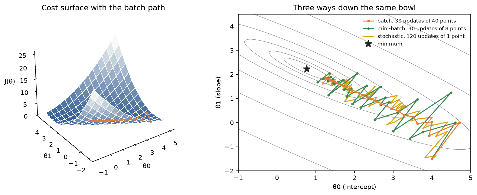
The figure shows the cost of 40 points around y = 1 + 2x with x between 0 and 2, where κ = 23.0, all runs starting from (4, -1.5). Batch gradient descent with η = 0.6 zigzags across the valley at first and then follows its floor; after 30 updates its cost is 0.0197 above the minimum. Thirty mini-batch updates of 8 points and 120 stochastic updates of 1 point with η = 0.15 follow the same valley more noisily and end 0.1087 and 0.0444 above it, for a fraction of the work: 240 and 120 single-example gradients against 1,200.

How fast gradient descent converges

The cost is quadratic, and because the normal equation makes the linear term vanish at the minimum, it is exactly a bowl centred on θ̂ whose shape is the curvature matrix A:

The error e after t batch steps, the distance from θ̂, is therefore multiplied by I - ηA at every step. Write A in its orthonormal eigenvectors q with eigenvalues λ, and expand the starting error in them with coefficients c. Each component then evolves on its own:

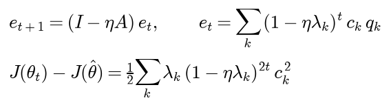
Three results follow.

• Stability. The iteration converges from every start exactly when each factor 1 - ηλk is smaller than one in absolute value:

Above the limit the steepest component grows by the factor |1 - ηλmax| per step and the cost explodes; just below it, that component flips sign every step and decays slowly.

• Rate. With η = 1/λmax the steepest direction is solved in one step and the flattest shrinks by the factor 1 - 1/κ per step. Every factor in the cost gap is then at most e to the power -2/κ, so the gap shrinks exponentially, and reaching a fraction ε of the starting gap takes a number of iterations proportional to κ:

For ε = 10⁻⁶ that is about 6.9κ. The best fixed rate, 2/(λmax + λmin), improves the factor to (κ - 1)/(κ + 1), which still means a number of iterations proportional to κ.

• Geometry. The level sets of J are ellipses, ellipsoids in higher dimensions, whose axes point along the eigenvectors with half-lengths proportional to 1/√λk. Their aspect ratio is √κ: a large condition number is a long narrow valley, across which gradient descent bounces while it creeps along the floor.

Feature scaling

Everything about the speed of gradient descent is in κ, and κ depends on the units of the features. For one feature with mean μ and variance s², the mean squared deviation, the curvature matrix and its eigenvalues are:

The approximation holds when 1 + μ² + s² is large. Shifting a feature away from zero or stretching it both make κ, and with it the number of iterations, grow quadratically. Centring (μ = 0) leaves A diagonal with entries 1 and s², so κ is the larger of s² and 1/s². Standardizing makes A the identity:

With a standardized feature κ = 1, every direction has the same curvature, and gradient descent with η = 1 reaches the minimum in a single step. With several standardized features A has a 1 for the intercept and the correlation matrix of the features in the rest, so what remains of κ comes from correlation between features, which scaling cannot remove. Scaling to [0, 1] by the minimum and maximum does not centre the data and leaves κ above one.

Scaling changes the path, not the destination: the second line of the formula above converts standardized parameters back, and the least-squares predictions are identical. The means and standard deviations must come from the training rows only; computing them on all the data leaks the test rows into the model, as Data leakage and pitfalls shows.

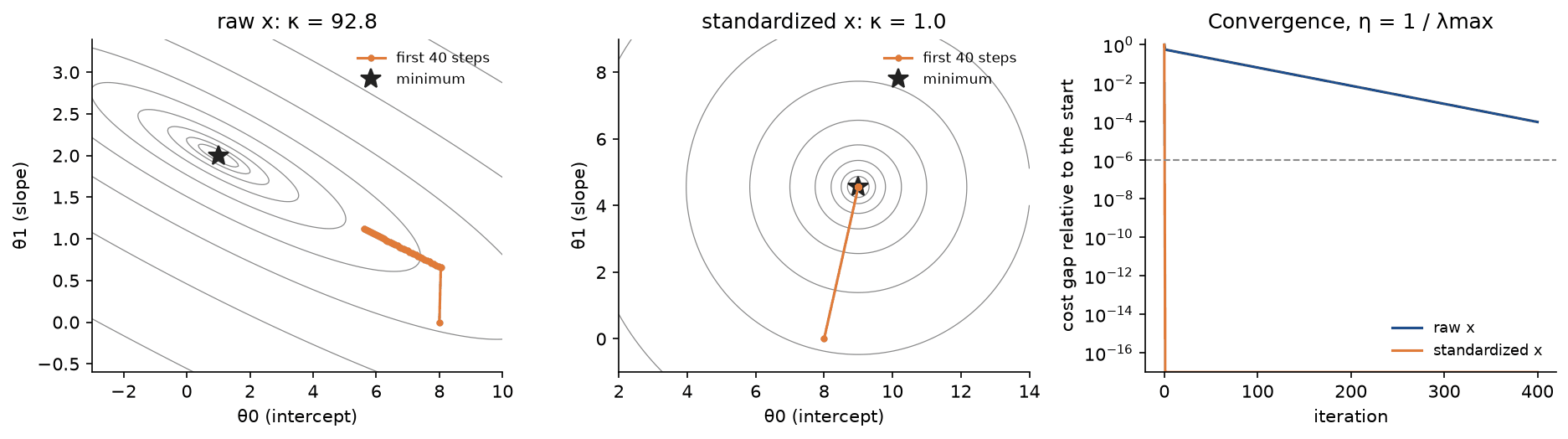
The figure runs the worked example below from (8, 0) with η = 1/λmax of each problem. On raw x, where κ = 92.8, the path reaches the valley floor in a few steps and then crawls along it; after 400 steps the cost gap is still about 10⁻⁴ of its start. On standardized x the contours are circles and one step lands on the minimum.

Polynomial and interaction features

The model only has to be linear in θ. Replacing x by x, x² and so on up to the power d fits a polynomial; adding a product of two features lets the effect of one depend on the other, an interaction. All monomials of degree 1 to d in n inputs number

because the monomials of degree at most d correspond to the ways of distributing d units among n variables and one slack position, and the constant is already in the design matrix. Eight inputs give 44 columns at degree 2, 164 at degree 3 and 494 at degree 4. Products of distinct inputs only, without squares, number the sum of n choose k for k from 1 to d.

Two cautions. Raw powers of an input are nearly parallel and of wildly different sizes, so the design matrix becomes badly conditioned; standardizing the generated columns keeps it usable. And the models are nested, since a degree d fit can set its top coefficient to zero, so training error can only fall as the degree rises, while error on new data falls and then rises again.

Indicator columns are features too. The sample project adds one column per small grid cell of latitude and longitude, equal to 1 for the block groups inside the cell and 0 elsewhere, which lets every neighbourhood have its own price level while the model stays linear.

Ridge regression

Ridge adds a penalty on the size of the slopes. Setting the gradient of the penalized sum of squares to zero gives a closed form:

The matrix is invertible for every λ > 0, even when the columns of X are dependent: vᵀ(XᵀX + λD)v is ‖Xv‖² plus λ times the sum of squares of v1 to vn, which is positive unless all of v1 to vn vanish, and then ‖Xv‖² = m v0² > 0 unless v = 0. In the cost-function form used for gradient descent the same problem adds λ times the squared slopes to RSS before dividing by 2m, and its gradient gains λDθ/m.

The intercept is left out of the penalty so that adding a constant to every target moves only θ0. Leaving it out is the same as centring: for fixed slopes the best intercept is ȳ - x̄ᵀw, and substituting it turns the problem into ridge without an intercept on centred data. This is the objective of scikit-learn's Ridge(alpha=λ).

The singular value decomposition of the centred features, with singular values σk and singular vectors uk and vk, shows what the penalty does:

Each direction vk is shrunk by the factor σk² / (σk² + λ). Directions with small singular values, the ones the data determine poorly and whose least-squares coefficients vary most from sample to sample, are shrunk most. The effective number of parameters df falls from n at λ = 0 towards 0, and one decomposition gives the whole path of solutions. Because the penalty treats all coefficients alike while their sizes depend on the units of their features, features are standardized before ridge is applied. Ridge is also the most probable θ under the Gaussian model above with a Gaussian prior on the slopes of variance σ²/λ. Regularization follows the same penalty into neural networks, where it is called weight decay.

The lasso and coordinate descent

The lasso penalizes absolute values instead, here in scikit-learn's scaling, with the squared error divided by 2m:

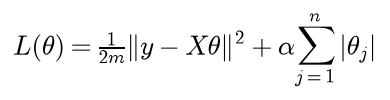
The absolute value has a corner at zero, so there is no closed form in general, but the problem is convex and easy in one coordinate at a time. Handle the intercept by centring as for ridge, fix every slope but one, and call the free slope t. With the partial residual that the other features leave, the objective is a parabola in t plus α|t|:

Here aj is the curvature of the cost along coordinate j, and ρj measures how strongly feature j lines up with the residual that the other features leave. Consider the three cases. For t > 0 the derivative is aj t - ρj + α, which vanishes at t = (ρj - α)/aj; that is positive only if ρj > α. For t < 0 the stationary point is (ρj + α)/aj, negative only if ρj < -α. If |ρj| ≤ α, neither side has a stationary point, the function decreases towards zero from both sides, and the minimum is at t = 0. Together:

Soft-thresholding moves ρj towards zero by α and stops at zero. Coordinate descent sweeps j = 1 to n repeatedly, and because the non-smooth part of L is a sum of terms in single coordinates, it converges to the minimum. Computing ρj from scratch costs a pass over all m examples. When there are many more examples than features it is cheaper to compute the Gram matrix G and the correlations c of the centred data once; then ρj needs only the vector Gw, which each update changes by one column of G:

The diagram is the whole algorithm in lasso.py. A sweep costs about n² operations instead of m n, which lets the sample project run a lasso path over 461 columns and 12,384 rows in a few seconds of plain Python. The optimality conditions follow from the same case analysis, and they say where the path begins:

The difference from ridge is clearest for orthonormal features, X̃ᵀX̃/m equal to the identity, where both have closed forms in terms of the least-squares slopes ŵj:

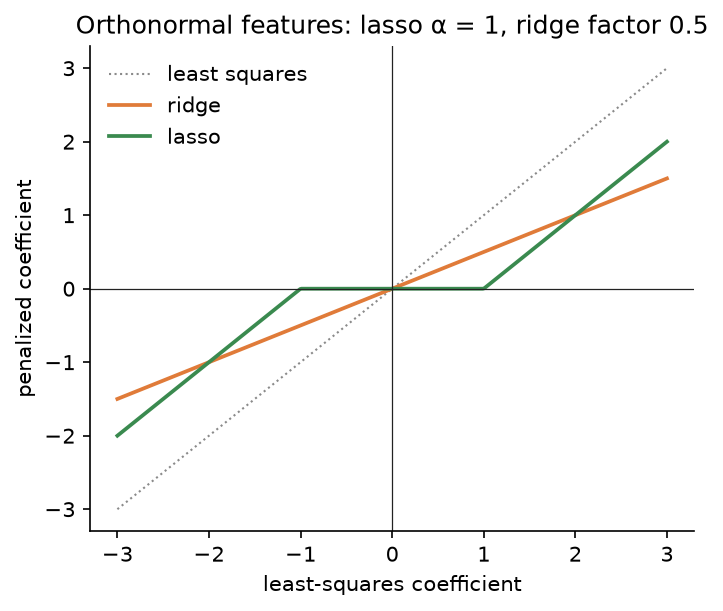
The lasso subtracts a fixed amount and clips at zero, so small coefficients become exactly zero and the model selects features; ridge shrinks every coefficient by the same factor and never reaches zero. The regularization path is computed for a decreasing grid of α starting at α_max, each fit starting from the previous solution; neighbouring solutions are close, so each warm-started fit needs few sweeps. Among strongly correlated features the lasso tends to keep one and drop the others, and which one it keeps can change with small changes in the data.

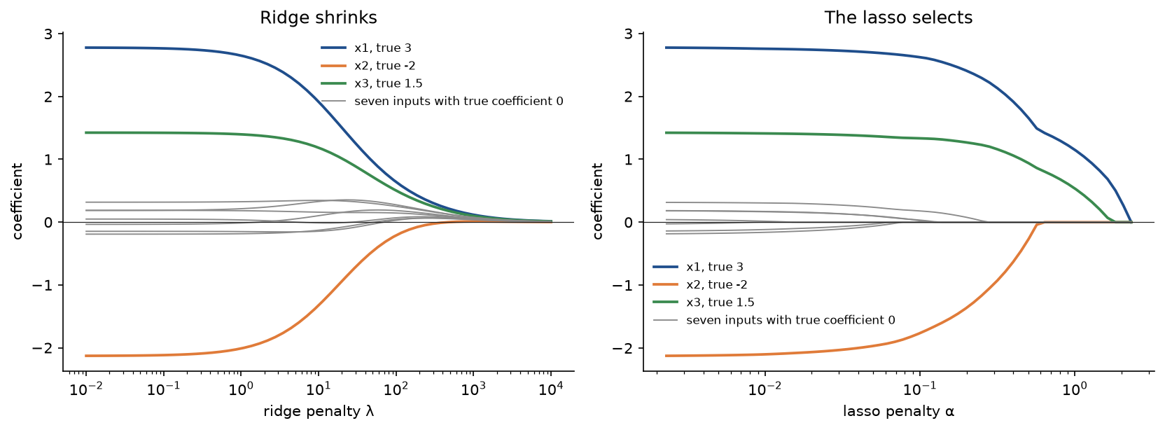
The figure fits 60 examples with ten inputs of pairwise correlation 0.5, of which three have true coefficients 3, -2 and 1.5. Ridge shrinks all ten smoothly, and its effective number of parameters falls from 9.63 at λ = 1 to 5.03 at λ = 30 and 1.26 at λ = 300. The lasso removes them one at a time from α_max = 2.3119 down: at α = 0.05 eight coefficients are non-zero, at 0.2 four and at 0.5 exactly the three useful inputs remain.

R-squared and adjusted R-squared

R-squared compares the residual sum of squares with the spread of the targets around their own mean:

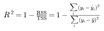
It is the share of the spread of the targets that the model removes. Predicting ȳ for every example gives RSS = TSS and R² = 0, a perfect fit gives 1. For a least-squares fit with an intercept, on its own training data, the decomposition TSS = ESS + RSS gives two equivalent forms, ESS/TSS and the squared correlation of y and ŷ, and guarantees R² between 0 and 1. On test data, or for a model without an intercept, the decomposition fails: 1 - RSS/TSS can be negative, which means worse than predicting the mean, while ESS/TSS can exceed one. The definition 1 - RSS/TSS, with the mean of the data being scored, is the one to use everywhere; it is what scikit-learn's r2_score computes.

The denominator is the spread of the observed targets. Writing the spread of the fitted values there instead is a different quantity. On a training fit with an intercept ESS = R² TSS and RSS = (1 - R²) TSS, so it equals

which is close to R² for good fits and goes negative whenever R² < 1/2.

Training R² never falls when a column is added, because the larger model contains the smaller one. Adjusted R² replaces both sums by unbiased variance estimates, dividing each by its degrees of freedom, with p the number of predictors:

Adding a predictor raises adjusted R² only if it lowers RSS by more than the degree of freedom it costs; precisely, when the absolute value of its t statistic exceeds one. It removes the average optimism of training R², but it estimates how much of the variance the best coefficients for those columns would explain, not how well the fitted coefficients will predict new data. For that, use held-out data; Evaluation metrics covers held-out evaluation and cross-validation.

Residuals and heteroscedasticity

A residual plot shows the residuals against the fitted values, or against a feature. Least squares makes the residuals average zero and leaves them uncorrelated with the fitted values, so a well-specified model leaves a structureless horizontal band. Typical patterns and what they mean:

• A curve or a wave means a nonlinearity the model cannot express. Add polynomial terms or transformed features, or use a different model.
• A funnel that widens with the fitted value means the noise variance grows with the level, which is heteroscedasticity. Log-transform a positive target, use weighted least squares, or use robust standard errors.
• A straight diagonal edge means the target is capped or censored. Use a model for censored data, or drop the capped rows knowingly.
• A few isolated points are outliers or high-leverage rows. Inspect them, and consider a robust loss.

Under heteroscedasticity the noise variance σi² varies from example to example. The least-squares estimate is still unbiased, but its covariance is a sandwich:

It reduces to the classical σ²(XᵀX)⁻¹ only when all the variances are equal. The classical standard errors, the square roots of the diagonal of σ̂²(XᵀX)⁻¹ with σ̂² = RSS/(m - n - 1), are then wrong: too small for coefficients of features whose large values carry large noise, and too large for others. The sandwich estimate replaces Σ by the diagonal matrix of squared residuals and stays valid. If the variances are known up to a constant, weighted least squares gives the most precise linear unbiased estimate; it is ordinary least squares on rows rescaled by the square roots of the weights, which makes the noise constant again:

weighted_least_squares solves this system, and classical_standard_errors and robust_standard_errors compute both kinds of standard error; the pitfall on heteroscedasticity below measures how far apart they drift.

Worked example

Five points with one feature: (1, 1), (2, 6), (4, 11), (6, 14) and (7, 13), so x = (1, 2, 4, 6, 7) and y = (1, 6, 11, 14, 13). Every value below is computed in double precision and shown to four decimals where it is not exact.

The normal equation

The design matrix has a column of ones and the column of x. Its normal equation needs m = 5, the sum of x, 20, the sum of x², 1 + 4 + 16 + 36 + 49 = 106, the sum of y, 45, and the sum of x y, 1 + 12 + 44 + 84 + 91 = 232. The determinant of XᵀX is 5 × 106 - 20² = 130, and Cramer's rule gives

The fitted line is ŷ = 1 + 2x. The centred formulas agree: x̄ = 4 and ȳ = 9, the deviations are (-3, -2, 0, 2, 3) and (-8, -3, 2, 5, 4), so S_xx = 26, S_xy = 24 + 6 + 0 + 10 + 12 = 52, the slope is 52/26 = 2 and the intercept 9 - 2 × 4 = 1.

Residuals and the projection

The fitted values are (3, 5, 9, 13, 15) and the residuals (-2, 1, 2, 1, -2). Both columns of X are orthogonal to the residuals, as the projection argument demands: their sum is -2 + 1 + 2 + 1 - 2 = 0 and their products with x add up to -2 + 2 + 8 + 6 - 14 = 0. The residuals form an arch, negative at both ends and positive in the middle, a first hint that a straight line misses some curvature.

Goodness of fit

• RSS = 4 + 1 + 4 + 1 + 4 = 14, TSS = 64 + 9 + 4 + 25 + 16 = 118 and ESS = 36 + 16 + 0 + 16 + 36 = 104, and indeed 104 + 14 = 118.
• R² = 1 - 14/118 = 0.8814, and the squared correlation of x and y is 52² / (26 × 118) = 0.8814 as well.
• Adjusted R² = 1 - (14/118) × 4/3 = 0.8418.
• The fitted-value denominator would give 1 - 14/104 = 0.8654, which equals (2R² - 1)/R².

Two steps of gradient descent

Start from θ = (0, 0) with η = 0.05. All predictions are zero, so the cost is the sum of squared targets over 10, 523/10 = 52.3, and the gradient is minus one fifth of Xᵀy:

• Step 1: the gradient is (-9, -46.4) and θ becomes (0.45, 2.32).
• At θ = (0.45, 2.32) the predictions are (2.77, 5.09, 9.73, 14.37, 16.69) and the errors ŷ - y are (1.77, -0.91, -1.27, 0.37, 3.69). The cost is (3.1329 + 0.8281 + 1.6129 + 0.1369 + 13.6161)/10 = 1.9327.
• Step 2: the errors sum to 3.65 and their products with x to 1.77 - 1.82 - 5.08 + 2.22 + 25.83 = 22.92, so the gradient is (0.73, 4.584) and θ becomes (0.4135, 2.0908), with cost 1.4464.

The minimum cost is 14/10 = 1.4. The first step removed almost all of the cost but overshot the slope, 2.32 against 2. The second pulled the slope back while the intercept, 0.4135 against 1, drifted further away: what remains is a slow walk along the floor of the valley, as the eigenvalues below explain. A stochastic step on the third example alone, x = 4 and y = 11, from the same start would use that example's gradient (0 - 11) × (1, 4) = (-11, -44) and move to (0.55, 2.2).

How many steps

The curvature matrix A = XᵀX/5 has rows (1, 4) and (4, 21.2), trace 22.2 and determinant 5.2, so its eigenvalues are

so κ = 92.7661 and the largest stable learning rate is 2/λmax = 0.0911. With η = 0.05 the steep direction is multiplied by 1 - 0.05 × 21.9632 = -0.0982 per step, nearly removed at once with a slight overshoot, and the flat direction by 0.9882, which is why the first step did most of the work and the rest is slow. With η = 1/λmax the bound promises a cost gap of 10⁻⁶ of the starting gap within ⌈92.7661/2 × ln 10⁶⌉ = 641 iterations; the measured number is 312.

Standardizing x with μ = 4 and s = √(26/5) = 2.2804 gives z = (-1.3156, -0.8771, 0, 0.8771, 1.3156), whose sum is 0 and sum of squares 5, so A becomes the identity. One step with η = 1 from zero lands on the minimum: θ becomes (sum of y, sum of z y)/5 = (9, 4.5607), which converts back to the slope 4.5607/2.2804 = 2 and the intercept 9 - 2 × 4 = 1.

Ridge and the lasso

Ridge with λ = 6.5 adds 6.5 to the slope entry of XᵀX:

The first row gives θ0 = 9 - 4θ1; substituting into the second, 180 + 32.5 θ1 = 232, so θ1 = 1.6 and θ0 = 2.6. In centred form the slope is S_xy / (S_xx + λ) = 52/32.5: ridge multiplied the slope by 26/32.5 = 0.8.

The lasso with α = 2.6 needs one coordinate update, since there is only one slope. On centred data ρ = S_xy/m = 10.4 and a = S_xx/m = 5.2, so

The lasso subtracted α/a = 0.5 from the slope instead of scaling it, and from α_max = 10.4 on the slope is exactly zero and the model predicts 9 everywhere. Both penalized lines still pass through the point of means (4, 9) because the intercept is free.

A quadratic feature

Adding the column x² gives a three-column design matrix. XᵀX has rows (5, 20, 106), (20, 106, 632) and (106, 632, 3970), Xᵀy = (45, 232, 1342), and the solution is θ = (-29/7, 122/21, -10/21) = (-4.1429, 5.8095, -0.4762). The residuals become (-4, 9, -10, 9, -4)/21, so RSS = 294/441 = 0.6667, R² = 0.9944 and, with p = 2, adjusted R² = 1 - (0.6667/118) × 4/2 = 0.9887. Adjusted R² rises from 0.8418 to 0.9887, so the extra parameter more than pays for itself. With five points that is all the evidence there is; on real data the comparison would be made on held-out rows.

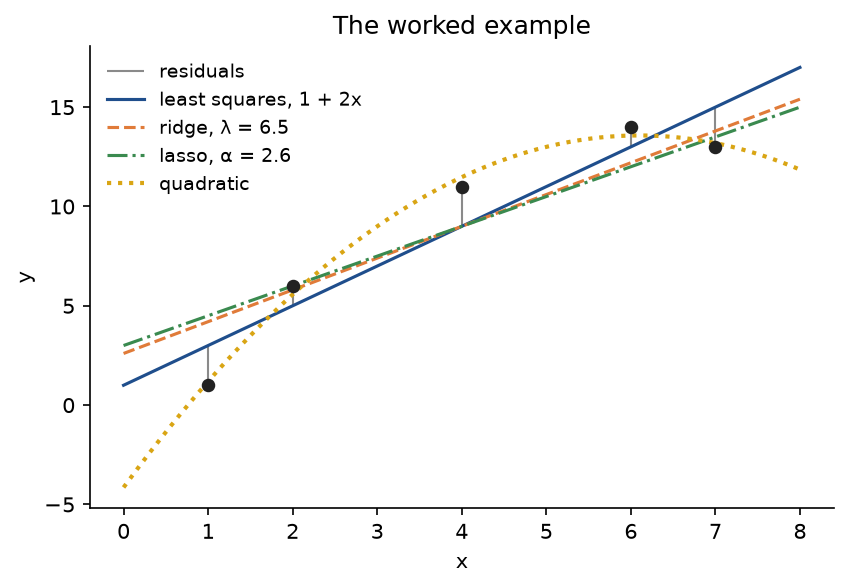
The figure shows why the penalized lines pivot around (4, 9): with a free intercept, shrinking the slope can only rotate the line about the point of means. Every number in this section is asserted by tests/test_trace.py and printed by examples/worked_fit.py.

The code

The package linear_regression is plain NumPy, split into one module per idea. scikit-learn is imported only inside load_california_housing and the functions of comparisons.py. Every fitting function takes a design matrix whose column 0 is the column of ones and returns θ with the intercept first.

• arrays.py holds the array types, the shape checks and design_matrix, which adds the column of ones.
• solvers.py solves least squares exactly: normal_equation, least_squares_qr, least_squares_svd (minimum norm), simple_linear_regression and hat_matrix.
• metrics.py holds the sums of squares, the mean squared error and its root, r_squared and adjusted_r_squared.
• descent.py holds the cost, its gradient, a finite-difference check and gradient_descent for batch, mini-batch and stochastic updates with an optional ridge penalty and decaying rate.
• conditioning.py holds the curvature matrix, its eigenvalues, the condition number, the largest stable learning rate, the iteration bound and iterations_to_converge.
• features.py holds the Standardizer, which also converts parameters back to original units, and polynomial and interaction terms with their names.
• ridge.py holds ridge, ridge_path (one SVD for every penalty), effective_degrees_of_freedom and PolynomialRidge, a small pipeline of polynomial terms, standardization and ridge.
• lasso.py holds soft_threshold, the coordinate descent with Gram updates, lasso, lasso_alpha_max, lasso_objective and the warm-started lasso_path.
• inference.py holds weighted least squares, classical and robust standard errors and the residual spread in bins of the fitted value.
• datasets.py generates the synthetic data from seeds, splits rows reproducibly and downloads the California housing data.
• housing.py holds the feature engineering of the sample project: logarithms of the long-tailed features, location cells and HousingDesign, which learns cells and column statistics from the fitting rows only.
• selection.py scores ridge and lasso paths on validation rows and picks the best curve.
• trace.py holds worked_example and trace_fit, which keeps every number of the worked example, and report.py prints them.
• experiments.py holds the small experiments behind the figures and pitfalls, so the examples, the notebook and the tests report the same numbers.
• pitfalls.py holds deliberately wrong code: the explicit inverse, updating one parameter at a time, the fitted-value denominator, a penalized intercept and the one-hot trap.
• comparisons.py fits the same models with scikit-learn.
• plotting.py, descent_plots.py and diagnostic_plots.py draw every figure in the handbook's four colours and save it reproducibly.

The inner loop of the lasso in lasso.py is the soft-thresholding update with the residual correlation read from the vector Gw, written out for one number because that is much faster in a Python loop:

rho = correlations[index] - products[index] + curvature * old
if rho > alpha:
    new = (rho - alpha) / curvature
elif rho < -alpha:
    new = (rho + alpha) / curvature
else:
    new = 0.0
if new != old:
    products += gram[index] * (new - old)
    slopes[index] = new

The examples and the project import the package, so install the repository first as described in the main README. Each example demonstrates one idea and runs from the repository root:

• examples/worked_fit.py prints every value of the worked example in the order above and draws its figure.
• examples/gradient_descent.py runs batch, mini-batch and stochastic descent down the same bowl, sweeps the learning rate across its limit on the worked example, and compares a constant with a decaying stochastic rate.
• examples/feature_scaling.py transforms the worked example's feature six ways, then shows scaling, long tails and the three descent variants on the full California housing data in about ten seconds.
• examples/regularization.py fits polynomials of degree 1 to 15, an interaction, and the ridge and lasso paths of ten correlated inputs.
• examples/fit_diagnostics.py compares the two R-squared denominators, inflates training R-squared with noise columns, draws residual patterns and measures classical and robust standard errors in 2,000 simulated data sets.
• examples/common_mistakes.py demonstrates the explicit inverse, updating one parameter at a time, a penalized intercept, penalties in arbitrary units, penalty scales that differ between objectives and the one-hot trap.

python machine-learning/linear-regression/examples/worked_fit.py
python machine-learning/linear-regression/examples/gradient_descent.py
python machine-learning/linear-regression/examples/feature_scaling.py
python machine-learning/linear-regression/examples/regularization.py
python machine-learning/linear-regression/examples/fit_diagnostics.py
python machine-learning/linear-regression/examples/common_mistakes.py

The sample project: house prices in California

project/house_prices.py predicts the median house value of Californian census block groups. It holds out a fifth of the rows as a test set, splits the rest into rows for fitting and rows for validation, compares a least-squares baseline with engineered feature designs, lets validation choose between ridge and the lasso and their penalties, refits the choice on all training rows and touches the test rows exactly once. It ends with residual diagnostics, the lasso path of the eight features and a check against scikit-learn.

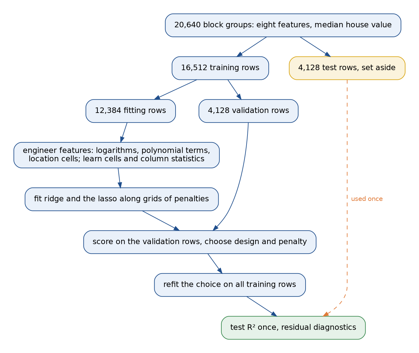
The cells of the location grid and the means and standard deviations of every column are learned inside the fitting rows only, so the validation and test rows never shape the features that score them. Options such as --seed, --max-degree and --cell-size change the setup, and --figures sends the three PNGs to another folder so a custom run does not overwrite the ones shown here. The default run takes about 25 seconds.

python machine-learning/linear-regression/project/house_prices.py
python machine-learning/linear-regression/project/house_prices.py --cell-size 0.5 --figures /tmp/figures

The data hold 20,640 block groups, of which 965 have the target at the cap of 5.00001, that is 500,001 dollars, where every larger value was recorded. Least squares on the eight raw features explains 0.6374 of the test variance, with a test RMSE of 0.7048, about 70,000 dollars; its training R² is 0.5980 and its adjusted R² 0.5978. Median income dominates: one more unit, ten thousand dollars of median income, goes with about 43,000 dollars of house value at fixed values of the other features.

Three kinds of engineered features improve on it, each a set of new columns for the same least squares:

• Logarithms of the four long-tailed features (average rooms, bedrooms, population and occupancy) raise the validation R² of least squares from 0.6103 for the raw features to 0.6713.
• Polynomial terms of degree 2, 3 and 4 in those eight features, with 44, 164 and 494 columns, reach 0.7262, 0.7492 and 0.5697 without a penalty. Ridge barely changes the first two, because 12,384 rows determine 164 coefficients well, but rescues degree 4 to 0.7382 at λ = 10.
• One indicator per quarter-degree location cell: 453 cells in the fitting rows, with a median of three block groups each. With the intercept these columns are perfectly collinear, so λ = 0 gives the minimum-norm solution, and the penalty matters: with the eight features it lifts validation R² from 0.6946 to 0.7315, and with degree 3 terms, 617 columns in all, from 0.7676 to 0.7784, both at λ = 31.6.

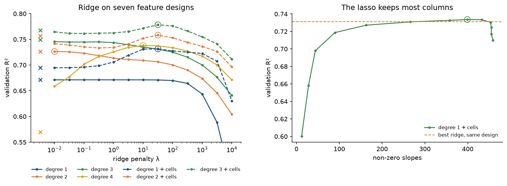
The left panel shows ridge working where the columns outnumber what the data can pin down, the degree 4 terms and the sparsely populated cells, and doing almost nothing elsewhere. The right panel asks the lasso to choose which cells deserve a level of their own: validation picks α = 0.0014, which keeps 399 of the 461 columns, 391 of the 453 cells, and scores 0.7336, level with ridge's 0.7315 on the same design. The price levels of neighbourhoods are many small effects rather than a few large ones, the situation ridge is built for, and the lasso honestly declines to make the model sparse.

Validation chooses ridge with degree 3 terms and location cells at λ = 31.6. Refitted on all 16,512 training rows, which visit 492 cells and give 656 columns, it reaches a test R² of 0.8039 and a test RMSE of 0.5183, against 0.6374 and 0.7048 for the baseline. For comparison, least squares with logarithms scores 0.6950 on the test rows, degree 3 terms without cells 0.7662, and the validated lasso with cells 0.7595. Every model scores a little higher on the test rows than on the validation rows, partly because the refit sees a third more rows and partly by the luck of the split; what matters is that the test rows played no part in any choice.

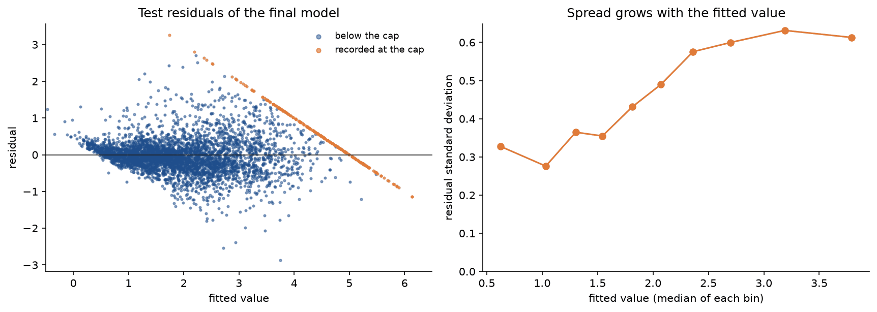
The residuals show what R² hides. The 207 test block groups at the cap fall on the line where the residual is 5.00001 minus the fitted value, a straight edge of slope -1. Leaving them out, the residual standard deviation grows from 0.328 and 0.276 in the two lowest tenths of the fitted values to 0.631 and 0.613 in the two highest, so the noise is heteroscedastic. For the raw baseline, the robust standard errors exceed the classical ones by a factor of 2.22 for median income, 2.54 for average rooms and 3.53 for average bedrooms; confidence intervals built from the classical formula would be far too narrow.

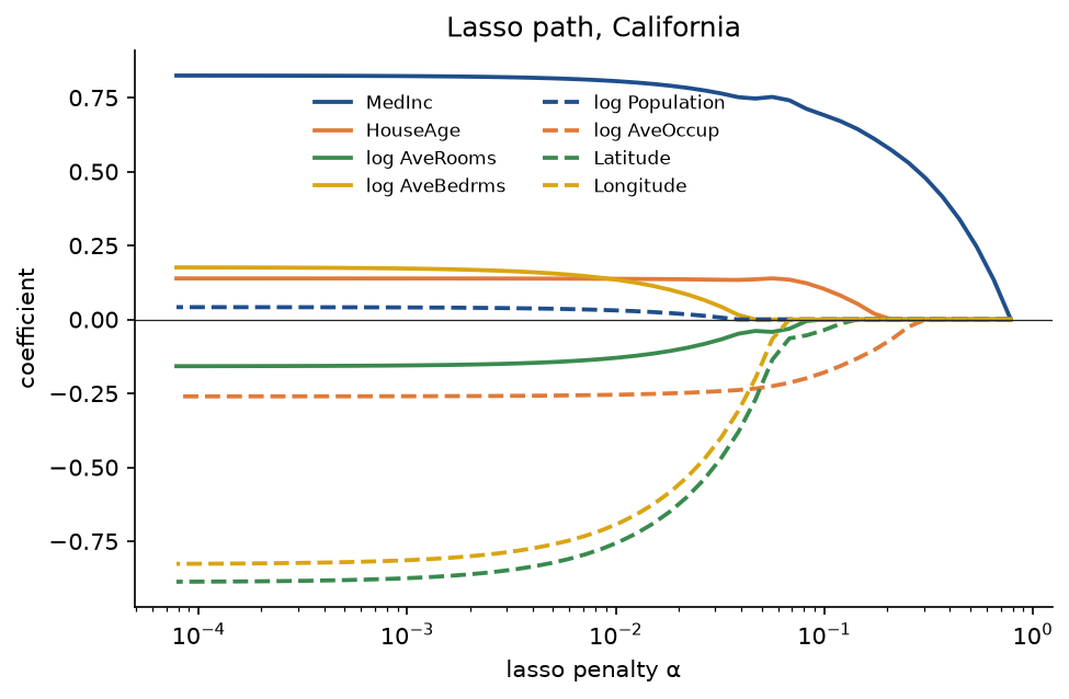
The lasso path on the eight standardized features with logarithms starts at α_max = 0.7839, where every slope is zero. Median income enters first, then log occupancy at α = 0.2538, house age, latitude, log rooms, longitude, log bedrooms and log population. At α = 0.1 four coefficients are non-zero and the test R² is 0.5753; at α = 0.01 all eight are in and it is 0.6914. Latitude and longitude enter late but end with the largest coefficients, about -0.89 and -0.83: the two are strongly correlated with each other, and each is useful mainly in combination with the other, which is the job the location cells do more directly.

The notebook linear_regression.ipynb is a guided tour in the order of this page: the worked example through trace_fit and again in bare NumPy, the cost surface, learning rates and scaling, polynomial and interaction features, ridge and lasso paths, R-squared and residuals, a demonstration of each pitfall, a short run on California housing and the comparison with scikit-learn. The tests in tests check the worked example value by value, the mathematical properties above and the agreement with scikit-learn, and run in a few seconds:

python -m pytest machine-learning/linear-regression

The synthetic data sets are generated from fixed seeds by the package. The California housing data set of R. K. Pace and R. Barry (1997) holds 20,640 block groups from the 1990 US Census, with eight features and the median house value. The underlying census figures are a work of the US federal government and in the public domain; the compiled table carries no separate licence and is redistributed by the StatLib archive and by scikit-learn. load_california_housing calls sklearn.datasets.fetch_california_housing, which downloads the archive once into .data/linear-regression/ at the repository root and verifies its pinned SHA-256 checksum before use. Nothing is committed.

In practice

For the same data and the same objective, scikit-learn gives the same answers. The sample project and the tests check each pair:

• Least squares: sklearn.linear_model.LinearRegression and numpy.linalg.lstsq agree with least_squares_qr to within 2.1 × 10⁻¹³ on the California coefficients.
• Ridge: sklearn.linear_model.Ridge(alpha=λ) agrees with ridge to within 1.5 × 10⁻¹² on the 656 columns of the final design.
• Lasso: sklearn.linear_model.Lasso(alpha=α) with tol=1e-12 agrees with lasso to within 2.9 × 10⁻¹², and sklearn.linear_model.lasso_path with lasso_path to within 8.9 × 10⁻¹⁰ over 50 values of α.
• Polynomial features: sklearn.preprocessing.PolynomialFeatures(include_bias=False) produces identical columns in the same order with identical names.
• Pipeline: make_pipeline(PolynomialFeatures, StandardScaler, Ridge) predicts within 7.9 × 10⁻⁶ of the degree 3 model fitted without a penalty. Its standardized design has a condition number above a million, and the two libraries solve it by different factorizations, so their rounding differs.
• R-squared: sklearn.metrics.r2_score computes the same 1 - RSS/TSS.

from sklearn.linear_model import Ridge

from linear_regression import random_problem, ridge

design, targets = random_problem(seed=14)
ours = ridge(design, targets, penalty=5.0)
library = Ridge(alpha=5.0).fit(design[:, 1:], targets)
print(ours[0] - library.intercept_, ours[1:] - library.coef_)

The library receives the features without the column of ones because it fits its own intercept, and its alpha is the λ of this page; the printed differences are of order 10⁻¹⁵. scikit-learn's SGDRegressor implements stochastic gradient descent with its own penalty scaling and learning-rate schedules and is not compared here. Standard errors, robust or classical, come from statsmodels (OLS(...).fit(cov_type="HC0") for the sandwich estimate), which is not a dependency of this repository; robust_standard_errors implements the same HC0 formula but is not tested against it.

When to use which:

• With up to a few thousand features and data that fit in memory, solve directly with LinearRegression or lstsq. The answer is exact and there is nothing to tune.
• With very many examples, streaming data or as a step towards models without a closed form, use mini-batch stochastic gradient descent on standardized features.
• With many correlated features or many small groups, such as the location cells, use ridge; RidgeCV chooses λ by an efficient leave-one-out formula.
• To select features, use the lasso with LassoCV, and check that the selection is stable; the elastic net mixes both penalties.
• For confidence intervals, use statsmodels with robust standard errors.

examples/feature_scaling.py shows gradient descent at the size of the California data. With η = 1/λmax on the raw features, κ = 5.707 × 10¹⁰ and the bound puts a cost gap of 10⁻⁶ some 3.9 × 10¹¹ iterations away; after 20,000 iterations the gap is still 0.148 of its start and the test R² is 0.0381. Standardized, the same problem has κ = 44.7, a bound of 310 iterations and converges in 169; after 200 iterations the test R² is the least-squares 0.6374, and after 3,000 the coefficients converted back to raw units agree with QR to 5.7 × 10⁻¹⁴.

Standardizing does not tame long tails. Average occupancy has a median of 2.8 but reaches 1,243 in one training row, 107 standard deviations above the mean, and that row's squared norm, 11,469, makes any stochastic step on it with η above 1.7 × 10⁻⁴ overshoot. Stochastic gradient descent with η = 0.001 diverges: the cost gap is 2.45 after the first epoch, 127 after the second and 6,665 after the third. Replacing the four long-tailed features by their logarithms shrinks the largest squared row norm to 590, lets the same run converge and raises the test R² of least squares to 0.6950.

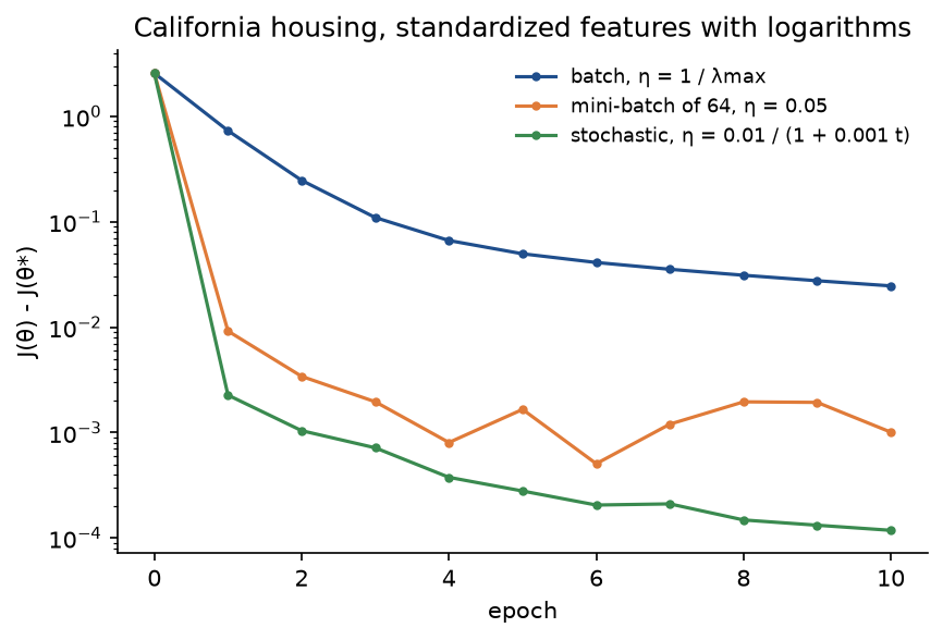
On these features, one epoch is one update for batch descent with η = 1/λmax, 258 updates for mini-batches of 64 with η = 0.05 and 16,512 for single examples with η = 0.01/(1 + 0.001 t). After one epoch their cost gaps are 0.731, 0.00918 and 0.00227, after ten 0.0246, 0.00101 and 0.000118. Per pass over the data, cheap noisy updates win by orders of magnitude, which is why stochastic methods train almost every large model.

Pitfalls

• The wrong denominator in R-squared. R² = 1 - RSS/TSS divides by the spread of the observed targets around their mean. A version that circulates in some notes divides by the spread of the fitted values. On a training fit with an intercept that gives (2R² - 1)/R²: 0.8654 instead of 0.8814 for the worked example, and -8.6222 instead of 0.0941 for a weak fit of 200 points (examples/fit_diagnostics.py, tests/test_pitfalls.py).
• Trusting training R-squared. Adding columns can only raise it. With 40 training rows, two useful inputs and 25 added pure-noise columns, training R² rises on average from 0.5716 to 0.8662 while R² on fresh data falls from 0.5191 to -0.5639; adjusted R² moves only from 0.5484 to 0.5651, which removes the inflation but does not reveal the collapse. Judge a model on held-out data.

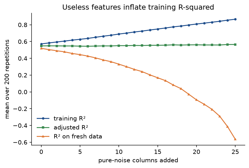
The three curves start together and part ways with every useless column, which is the whole case for held-out evaluation.

• Reading R-squared as bounded by zero and one. That holds only for a least-squares fit with an intercept on its own training data. On test data a model worse than the mean has negative R²; without an intercept even the training R² can be negative (tests/test_metrics.py).
• Inverting the normal equations. Forming XᵀX squares the condition number, and an explicit inverse adds its own rounding error. For a degree 11 polynomial in raw powers of an input between 0 and 10, the condition number of X is 1.4 × 10¹³ and that of XᵀX around 10²⁵, far beyond double precision. The explicit inverse gives an RSS of 91.2 against the optimum 3.1272, a number made of rounding error that changes from machine to machine; solving the normal equations misses the optimum in the fifth decimal, and QR and the SVD reach it (examples/common_mistakes.py). Use lstsq, QR or the SVD, and standardize generated features, which brings the condition number of X down to 8.9 × 10⁷.
• Updating parameters one at a time. Gradient descent computes every partial derivative at the same point and then updates all parameters. Updating θ0 first and using it for θ1's derivative gives (0.45, 2.23) instead of (0.45, 2.32) on the worked example. Some presentations of the update rule never say that the updates must be simultaneous; vectorized code, θ minus η times the gradient, does it automatically.
• A learning rate above the limit. Batch gradient descent diverges for η above 2/λmax. On the worked example the limit is 0.0911: at 0.093 the cost gap grows from 50.9 to 4.0 × 10⁴ in 80 steps, and at 0.09, just below the limit, the steep direction oscillates and decays so slowly that the run ends with a gap of 1.17, worse than the 0.0299 of η = 0.01 (examples/gradient_descent.py).

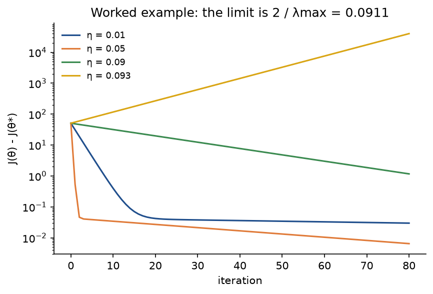
The best rate here, 0.05, is about half the limit: close enough to the limit to move the flat direction quickly, far enough to damp the steep one.

• Gradient descent on unscaled features. The number of iterations grows with κ, and κ grows quadratically with a feature's offset and scale. For the worked example's single feature, with η = 1/λmax and a target gap of 10⁻⁶ of the start:

• raw x: κ = 92.8, bound 641, measured 312 iterations;

• x + 10: κ = 7,860.5, bound 54,299, measured 44,923;
• 10x: κ = 8,649.2, bound 59,747, measured 33,639;
• min-max scaled to [0, 1]: κ = 11.4, bound 79, measured 62;
• centred x: κ = 5.2, bound 36, measured 32;
• standardized x: κ = 1.0, bound 7, measured 1.

Every version has the same least-squares fit (tests/test_experiments.py). On California housing the raw features would need hundreds of billions of iterations, the standardized ones 169. Fit the scaler on the training rows only, apply the same scaler at prediction time, and convert coefficients back with theta_to_original if they are to be read in original units; the scaling figure under How it works shows the two paths. - Outlying rows and stochastic gradient descent. Standardization fixes the average curvature, not single rows. A stochastic step on row i overshoots when η exceeds 2 divided by the squared norm of the row; on California housing one row with a standardized average occupancy of 107 makes stochastic gradient descent diverge at η = 0.001 until the long-tailed features are log-transformed (In practice, examples/feature_scaling.py). - A constant learning rate in stochastic gradient descent. The iterates keep jittering around the minimum: on the 40 points of the cost-surface figure, standardized, their distance from it is still 0.0894, 0.0853 and 0.1792 after 50, 100 and 200 epochs at η = 0.1, against 0.0007, 0.0001 and 0.0003 with η = 0.1/(1 + 0.01 t) (examples/gradient_descent.py). - Penalizing the intercept. Then adding a constant to every target changes the slopes: adding 100 to the targets of a two-feature ridge fit with λ = 20 moves its slopes from (2.0141, -0.5471) to (2.1696, 0.4576), while with a free intercept they stay at (2.0143, -0.5458) (examples/common_mistakes.py). - Regularizing unscaled features. Expressing one feature in thousandths changes the ridge fit with λ = 5, by up to 3.56 in a prediction, while least-squares predictions change only by rounding error (tests/test_pitfalls.py). Standardize before ridge or the lasso. - One number, two penalties. scikit-learn's Ridge(alpha) penalizes the sum of squared errors, while Lasso(alpha) and ElasticNet(alpha) penalize the mean squared error divided by two. ElasticNet(alpha=0.1, l1_ratio=0) on 60 rows is Ridge(alpha=6), not Ridge(alpha=0.1): the first three slopes are (2.1744, -1.5662, 1.2714) for both, against (2.7663, -2.1173, 1.4222). Check the objective before transferring a penalty value between libraries or papers. - Perfect collinearity. One-hot columns for all levels of a category add up to the column of ones, so XᵀX is singular. NumPy's solver does not even complain: rounding makes the matrix look invertible, with a condition number of 4.6 × 10¹⁶, and it returns one arbitrary member of the infinite solution set, (-0.15, 3.1167, 5.15, 7.25). The minimum-norm solution is (3.7667, -0.8, 1.2333, 3.3333), ridge with λ = 0.01 gives (5.0222, -2.0487, -0.0222, 2.0709) and dropping the first level gives (2.9667, 2.0333, 4.1333). The fitted values agree to 2.7 × 10⁻¹⁵ in every case, the coefficients do not. Drop one level, use the minimum-norm solution or add a penalty, as the sample project does for its location cells, and never read the coefficients of a collinear design. - Too high a polynomial degree, and extrapolation. With 20 training points, training RMSE falls from 0.5426 at degree 1 to 0.1100 at degree 15, below the noise level of 0.3, while the RMSE on fresh points is lowest at degree 5, 0.3737, and reaches 19.6 at degree 15. Outside the training range, which ends at x = 2.610, the degree 15 fit predicts about -260 at x = 3, where the true value is 0.222 (examples/regularization.py).

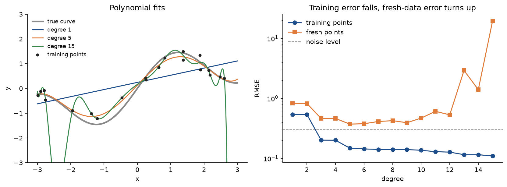
The degree 15 curve passes close to every training point and nowhere near the truth between and beyond them; its last digits depend on rounding, because its standardized design is still nearly singular.

• Ignoring heteroscedasticity. When the noise grows with a feature, the slope is still estimated without bias, but its classical standard error is wrong. In 2,000 simulated data sets of 200 points with noise standard deviation 0.2 + 0.04x², the slope's actual spread is 0.0601, the average classical standard error 0.0474 and the average robust one 0.0576; for the intercept the classical error, 0.2742, overstates the actual 0.1874 (examples/fit_diagnostics.py). Plot the residuals and use robust standard errors.

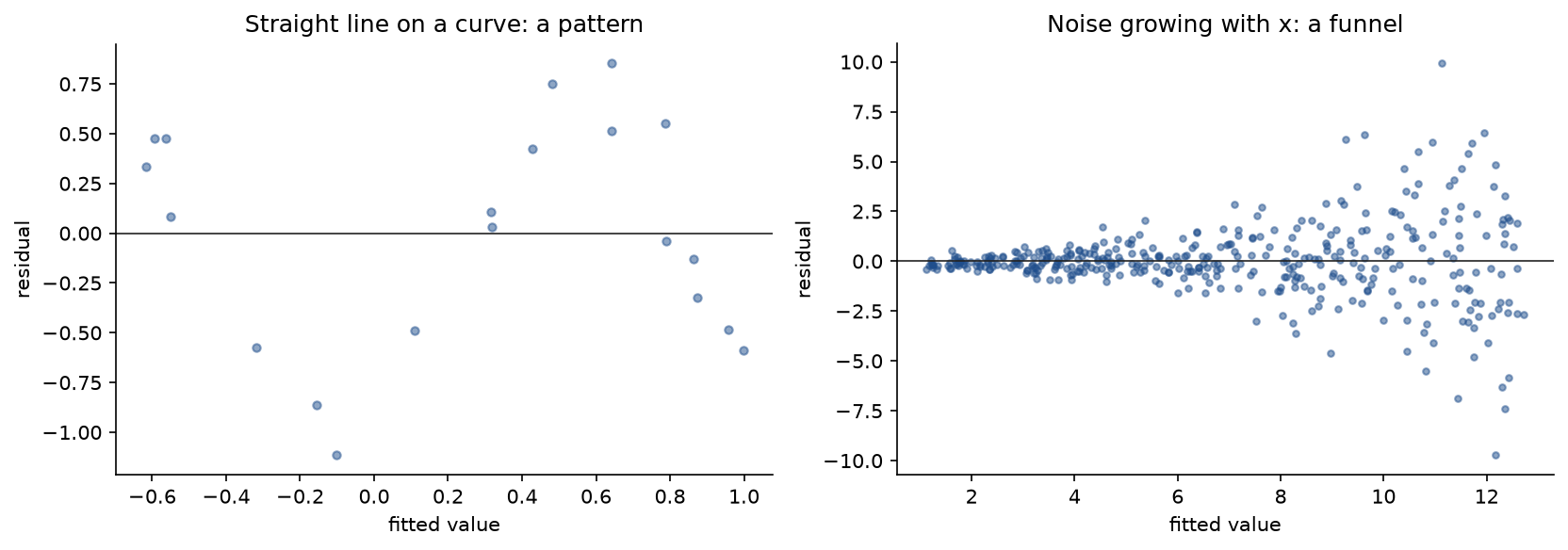
Neither pattern changes R² much, which is why the residual plot comes before any number.

Further reading

• T. Hastie, R. Tibshirani and J. Friedman, The Elements of Statistical Learning, second edition, Springer, 2009, chapter 3. Least squares, ridge, the lasso and their paths.
• G. James, D. Witten, T. Hastie and R. Tibshirani, An Introduction to Statistical Learning, second edition, Springer, 2021, chapters 3 and 6. A gentler treatment with residual diagnostics.
• A. E. Hoerl and R. W. Kennard, "Ridge regression: biased estimation for nonorthogonal problems", Technometrics 12(1), 55-67, 1970.
• R. Tibshirani, "Regression shrinkage and selection via the lasso", Journal of the Royal Statistical Society, Series B 58(1), 267-288, 1996.
• J. Friedman, T. Hastie and R. Tibshirani, "Regularization paths for generalized linear models via coordinate descent", Journal of Statistical Software 33(1), 1-22, 2010. Coordinate descent with soft-thresholding, covariance updates and warm starts, the method behind scikit-learn's Lasso.
• P. Tseng, "Convergence of a block coordinate descent method for nondifferentiable minimization", Journal of Optimization Theory and Applications 109(3), 475-494, 2001.
• G. H. Golub and C. F. Van Loan, Matrix Computations, fourth edition, Johns Hopkins University Press, 2013, chapter 5. QR, the SVD and the conditioning of least squares.
• L. N. Trefethen and D. Bau, Numerical Linear Algebra, SIAM, 1997, the parts on least squares and conditioning.
• S. Boyd and L. Vandenberghe, Convex Optimization, Cambridge University Press, 2004, section 9.3. Convergence of gradient descent and the role of the condition number.
• L. Bottou, F. E. Curtis and J. Nocedal, "Optimization methods for large-scale machine learning", SIAM Review 60(2), 223-311, 2018. Stochastic gradient methods and step-size schedules.
• H. White, "A heteroskedasticity-consistent covariance matrix estimator and a direct test for heteroskedasticity", Econometrica 48(4), 817-838, 1980. The sandwich estimate.
• R. K. Pace and R. Barry, "Sparse spatial autoregressions", Statistics and Probability Letters 33(3), 291-297, 1997. The source of the California housing data.