k-nearest neighbours

The k-nearest-neighbour rule labels a new example by finding the k most similar labelled examples and letting them vote, or, for regression, by averaging their targets. There is no training step and no assumed shape for the decision boundary, which makes it the simplest serious classifier and a standard baseline. Everything therefore rests on what "similar" means: the distance, the scale of each feature, the size of the neighbourhood and the dimension of the space. This page defines the classifier and the regressor, compares five distances on a query worked by hand, shows a change of units changing the answer, derives the bias-variance trade-off behind the choice of k, explains why distances stop discriminating in high dimension, builds and searches a KD-tree from scratch, states the 1-NN error bound and checks every piece against scikit-learn, ending with a handwritten digit recognizer. Afterwards you will be able to compute a k-NN prediction on paper, choose k and a distance by cross-validation, decide when to scale features and when a tree index pays off, and recognize when nearest neighbours are the wrong tool. It uses the cross-validation of Evaluation metrics.

To run the code in this topic, install the base group, and the ml group for scikit-learn, which supplies the digits data and the reference implementations.

Intuition

To guess the variety of a bean pod, find the pods you already know that look most like it and go with the majority. That is the whole method. Three choices decide how well it works:

• What "like" means. A distance turns two feature vectors into one number. Different distances rank the same training points differently, and every distance silently weighs features by their numeric range, so the unit a feature happens to be recorded in can decide the answer.
• How many neighbours vote. One neighbour copies the label of the single closest example, noise included; very many neighbours average over a region so large that the answer no longer depends on where the query is. Somewhere in between is a k that balances the two, and cross-validation finds it.
• How the votes count. Every neighbour can count equally, or closer neighbours can count more. Either way ties need a rule.

The method is called lazy because it postpones all work to prediction time: fitting just stores the training set, and each prediction compares the query with the stored examples. It is called non-parametric because it has no fixed set of parameters that summarize the data; the stored examples are the model, so its capacity grows with the data. Both properties cut both ways. No information is lost to a summary, but memory grows with the training set and a naive prediction costs one distance computation per stored example. Index structures such as the KD-tree reduce that cost in low dimension, and the curse of dimensionality explains why they, and the method itself, struggle in high dimension.

The diagram is the whole algorithm. The blue path computes every distance; the amber path is the KD-tree, which finds exactly the same neighbours while computing fewer distances when the dimension is low. Scaling sits before both because it changes which points are nearest.

How it works

Notation

The training set holds n examples with d features each, and q is the query, the point to predict. Example i is a vector x with label or target y. A distance between two vectors a and b is written ρ(a, b). Sorted by their distance from q, the training examples are x(1), x(2) and so on, with labels y(1), y(2), so x(1) is the nearest. N, written N with subscript k in the formula images, is the set of indices of the k nearest examples. The classes are numbered c = 1 to C, w is the weight of a neighbour's vote, and the bold 1 of a condition is 1 when it holds and 0 otherwise. With two classes, η(x) is the probability of class 1 at x, and R* is the Bayes error, the lowest error rate any classifier can reach. The formula images write the feature index as a subscript, for example a with subscript j for feature j of the vector a; the text writes "feature j of a".

The classifier and the regressor

The classifier predicts the class with the largest total vote among the k nearest training examples, with every weight equal to 1 for uniform voting:

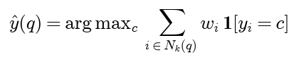
Dividing each class's vote by the total weight W gives class shares, which estimate the probabilities of the classes in a small neighbourhood of q. They are what predict_proba returns:

The regressor predicts the weighted mean of the neighbours' targets:

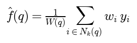
Both are local averages: the classifier averages indicators of class membership, the regressor averages targets. With k = 1 the classifier gives every query the label of the training point whose Voronoi cell contains it, the region closer to that point than to any other, so its decision boundary is made of Voronoi cell walls between differently labelled points. With k = n every query gets the overall majority class or the overall mean.

Distances

For p ≥ 1 the Minkowski distance of order p is

The power p applies to every absolute difference inside the sum and the root 1/p to the sum as a whole. Three orders have names:

In the plane their unit balls are a diamond, a circle and a square. The Chebyshev distance is the limit of the family. With M the largest absolute difference, the sum has d terms, none larger than M to the power p and at least one equal to it, so

and d to the power 1/p tends to 1 as p grows. Between these limits the distance never increases with p. Small p adds up every difference, so it favours points that differ in one coordinate only; large p looks only at the worst coordinate, so it favours points that differ a little in every coordinate. The worked example shows both effects changing the neighbours.

A metric satisfies four axioms:

Every Minkowski distance with p ≥ 1 is a metric; its triangle inequality is Minkowski's inequality. For 0 < p < 1 the formula still defines a dissimilarity, and scikit-learn accepts it, but the triangle inequality fails. For a = (0, 0), b = (1, 0), c = (1, 1) and p = 1/2:

Ball trees prune with the triangle inequality, which is why scikit-learn falls back to brute force for p < 1. The box bound of a KD-tree, described below, needs only that the distance grows with every coordinate difference.

The cosine similarity and the cosine distance compare directions:

The cosine distance lies between 0 and 2. Scaling either vector by a positive number leaves it unchanged, so all points on a ray from the origin are at cosine distance zero from each other. That is what makes the cosine right for word counts or embeddings, where the length of a vector mostly reflects the length of a document, and wrong for positions measured from an arbitrary origin. It is not a metric: distinct points can be at distance zero, and for u = (1, 0), v = (1, 1) and w = (0, 1) the distance from u to w is 1, more than the 2(1 - 1/√2) = 0.5858 of the detour through v. For unit vectors, expanding the squared Euclidean distance gives

so the Euclidean distance between rows normalized to unit length ranks neighbours exactly as the cosine distance does. That identity is how cosine search runs on Euclidean indices.

Feature scaling

The squared Euclidean distance is a sum of one term per feature. Recording feature j in a unit s times smaller multiplies its differences by s and its term by s², so a feature measured in large numbers dominates the distance regardless of how informative it is:

The choice of units is therefore a choice of metric, a weighted Euclidean distance with weights s². Standardization removes the arbitrary part of that choice. With μ and σ the mean and the standard deviation of feature j over the training set,

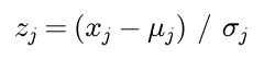
If the feature is re-expressed as s times x plus t with s > 0, its mean and standard deviation change with it and the standardized value does not:

Standardized coordinates, and every distance computed from them, do not depend on the units. Min-max scaling to [0, 1] achieves the same with the range in place of the standard deviation and is more sensitive to outliers. The Mahalanobis distance, with Σ the covariance matrix of the features, also removes correlations between them:

Standardization gives every feature the same spread and so the same say. That is right when the units are arbitrary and wrong when the features share a unit and their spreads carry meaning, as the pixel intensities of an image do; Pitfalls has a measured example. The statistics must come from the training rows only, inside every cross-validation fold, as Data leakage and pitfalls explains.

Choosing k: bias and variance

The trade-off can be derived exactly for regression. Suppose each target is f(x) plus independent noise ε of mean 0 and variance σ², and hold the training inputs fixed, so the neighbours of a query are fixed too. With uniform weights the estimate splits into the average of f over the neighbours and the average of their noises:

The second term has mean 0 and, as an average of k independent noises, variance σ²/k. Expanding the square around the first term, the cross term has mean zero, so

and the expected squared error on a new observation at q adds the irreducible σ². The variance falls like 1/k. The bias is the gap between the function at the query and its average over the neighbours; it is close to zero while the neighbours sit close to q and grows as larger k reaches farther away. Small k means low bias and high variance, large k the reverse, and the best k balances them. For classification the same picture holds without a closed form: k = 1 draws a ragged boundary around individual, possibly mislabelled points, and large k smooths the boundary until it misses real structure.

The training error cannot choose k. At k = 1 every training point is its own nearest neighbour and the training error is zero, unless identical inputs carry different labels. Cross-validation estimates the error on new data instead: split the training set into folds, predict each fold from the others for every candidate k, and average. The neighbours for k are the first k of the neighbours for the largest k, so one neighbour search per fold yields the predictions for every smaller k through running vote counts; cross_validation_errors works that way. The minimum of a cross-validation curve is itself a noisy estimate. The one-standard-error rule picks the simplest model, here the largest k, whose cross-validation error lies within one standard error of the minimum.

Choosing k on data with a known answer

examples/choosing_k.py measures all of this on synthetic data whose best possible error is known. Each class is an equal mixture of three round Gaussian blobs with standard deviation 0.55, and because the densities are known, the Bayes error can be computed: R* = 0.1364, averaged over 400,000 draws. With 400 training points, k = 1 has a test error of 0.1938 on 5,000 fresh points, k = 25 follows the best boundary closely at 0.1444, and k = 125 averages over almost a third of the data and reaches 0.4106.

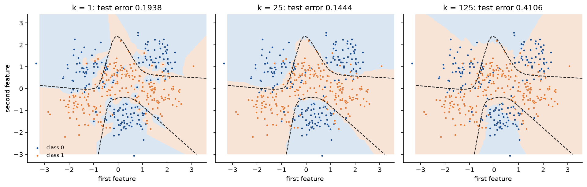
The regions show variance on the left and bias on the right. At k = 1 the boundary wraps around single points of the wrong class; at k = 125 whole blobs of class 0 disappear because their neighbourhoods reach into the more numerous class 1 around them.

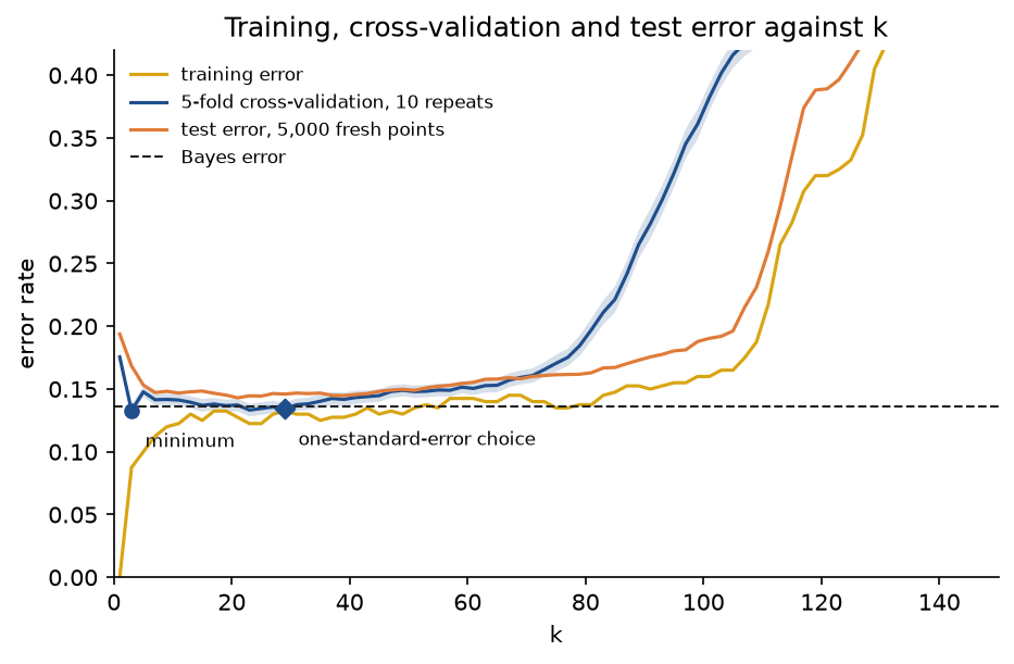
Five-fold cross-validation repeated with ten shuffles has its minimum, 0.1328 with a standard error of 0.0045, at k = 3, where the test error is 0.1684. The one-standard-error rule chooses k = 29, with a test error of 0.1460; the best test error over all k is 0.1430, at k = 21. The curve is flat over a wide range, so its minimum moves around from sample to sample: on ten independent training sets of 400 points the minimum rule chose k between 17 and 53 and the one-standard-error rule between 21 and 71, yet the test error at the chosen k was never more than 0.0052 above the best, and on average 0.0028 above it for the minimum rule and 0.0020 for the one-standard-error rule. The sample in the figure is an unlucky one for the minimum rule.

For regression the same example takes 100 noisy samples of sin x with noise σ = 0.3, computes both terms of the decomposition exactly on a grid of 200 queries with regression_risk, and checks their sum against 400 simulated redraws of the targets:

• k = 1: squared bias 0.0004, variance 0.0900, sum 0.0904, simulated 0.0890.
• k = 5: squared bias 0.0007, variance 0.0180, sum 0.0187, simulated 0.0181.
• k = 11: squared bias 0.0033, variance 0.0082, sum 0.0115, simulated 0.0112.
• k = 40: squared bias 0.0695, variance 0.0022, sum 0.0718, simulated 0.0721.

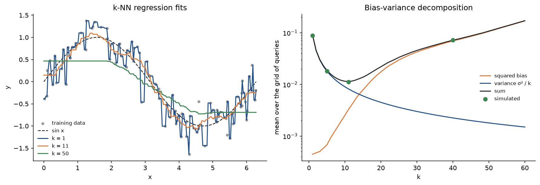
The expected squared error is smallest at k = 11. At k = 50 the fit flattens the peaks of the sine and runs flat at the ends of the range, where every query has the same one-sided neighbours: bias, measured.

Distance-weighted voting and ties

Distance weighting gives each neighbour the weight one over its distance, so close neighbours count more and the prediction changes smoothly as the query moves past a neighbour. Smoother kernels with a bandwidth h lead to kernel regression:

A training point at distance zero would get an infinite weight. The convention used by scikit-learn and here is that such points get weight 1 and all others weight 0. Ties arise in two places:

• Tied votes. With uniform weights, an even k and two classes, the vote can split evenly. An odd k prevents that for two classes but not for three or more. Common rules are: the smallest class label wins, which is what scikit-learn does because argmax returns the first maximum; the class of the nearest neighbour among the tied classes wins; a random class wins; or k is reduced by one until the tie disappears.
• Tied distances. When the k-th and the next nearest points are equally far away, one of them has to be left out. Our implementation keeps the lower training index, which makes brute force and the KD-tree agree exactly; libraries usually make no promise, and the result can change when the training rows are reordered.

The curse of dimensionality

Nearest neighbours work when the nearest points are much closer than typical points. In high dimension that stops being true. Take a query q and points x drawn uniformly from the unit cube in d dimensions. For one coordinate, with c the query's value there, the squared difference has the moments below; averaged over a uniformly placed c they become simple fractions:

The squared distance is a sum of d independent such terms, so for a typical query its mean is about d/6 and its standard deviation about √(d/30). The distance is the square root of the squared distance, and for a quantity with a small relative spread the square root halves the relative spread, so

The distances from a query to all points crowd into a band whose relative width shrinks like 1/√d: at d = 1000 it is 0.0173, so nearly every point is within a few percent of the same distance. The relative contrast, the farthest distance minus the nearest divided by the nearest, goes to zero with it, and "nearest" stops carrying information. Beyer and co-authors proved this concentration under much weaker conditions than uniformity. examples/high_dimensions.py measures it with 1,000 uniform points and 100 queries:

• d = 2: relative spread 0.4385 against the predicted 0.3873, relative contrast 107.5649.
• d = 10: spread 0.1800 against 0.1732, contrast 2.8198.
• d = 100: spread 0.0553 against 0.0548, contrast 0.4379.
• d = 1000: spread 0.0172 against 0.0173, contrast 0.1174.

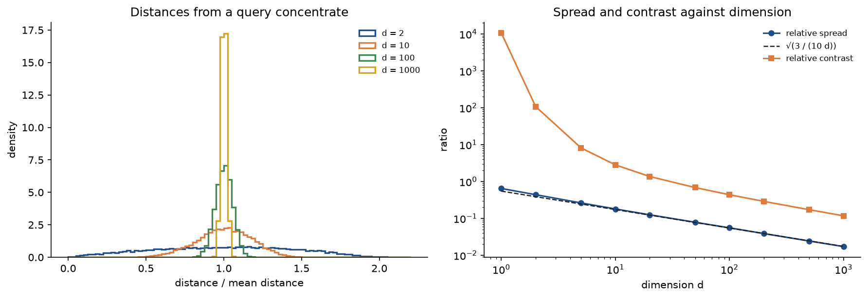
The approximation behind the formula needs many coordinates, which is why it is off in two dimensions. A second view of the same effect: a neighbourhood that contains a fraction r of uniformly spread data is a sub-cube with edge e, and

To capture 1 % of the data, the edge is 0.01 of the range in one dimension, 0.1 in two, 0.6310 in ten and 0.9550 in a hundred. A "local" neighbourhood in high dimension spans almost the whole range of every feature, and averaging over it is no longer local.

Real data often escape the worst of this because they lie near a low-dimensional set inside the feature space: 64-pixel digit images do not fill a 64-dimensional cube. What brings the curse back is irrelevant features. Each one adds noise to every distance without adding signal, and enough of them drown the informative ones. The same example adds features of uniform noise on [-2, 2] to the two informative mixture features and chooses k by cross-validation each time: the test error is 0.1684 with no noise feature, 0.1908 with 2, 0.2986 with 5, 0.4180 with 10, 0.4762 with 20 and 0.4866 with 100. Ten noise features push it most of the way to chance, 0.5. Feature selection, Dimensionality reduction or a learned embedding before the neighbour search are the remedies.

KD-trees

A KD-tree partitions the training points by recursive median splits so that a query can skip whole regions.

Construction. A node holds a set of points. If it holds at most leaf_size points it is a leaf. Otherwise choose a split coordinate, here the one with the widest spread (largest minus smallest value; the classic alternative cycles through the coordinates by depth), sort the points along it, send the first half, rounded down, to the left child and the rest to the right child, and record the coordinate of the first right point as the split value. Every node also stores the tightest box around its points, with lower corner ℓ and upper corner u. The tree has depth equal to log₂ of n over the leaf size, rounded up, and sorting at every level costs O(n log² n) in total, or O(n log n) with a linear-time median.

Search for the k nearest points of q. Keep the best k candidates found so far and let δ be the distance of the worst of them, infinite until k have been found. Visit nodes depth first, the child on the query's side of the split first. On reaching a leaf, compute the distances to its points and update the candidates. Before visiting any node, compute its box distance β, the distance from q to the nearest point of the box, which is zero when q lies inside it:

Every point z in the box is at least g j away from q in coordinate j, so no point in the box can be closer than the box itself:

If β exceeds δ, no point in the box can enter the candidate list, and the whole subtree is skipped without changing the answer. The search is exact; only the amount of work depends on the data. The bound holds for every Minkowski distance, and for the cosine distance only after normalizing the rows and switching to the Euclidean distance, as above.

Cost. For a fixed dimension and enough data, Friedman, Bentley and Finkel showed that the expected search time grows like log n, but the constant grows exponentially with d, because a small ball around the query can touch on the order of 2 to the power d cells. A rule of thumb is that a KD-tree helps when n is much larger than 2 to the power d. In high dimension the query ball crosses almost every splitting plane, the search visits almost every leaf, and the tree is slower than brute force because of its bookkeeping. Ball trees bound groups of points by spheres instead of boxes and cope somewhat better; for large high-dimensional collections, approximate methods (locality-sensitive hashing, graph indices such as HNSW, product quantization) trade exactness for speed, as used in Recommender systems and Retrieval-augmented generation.

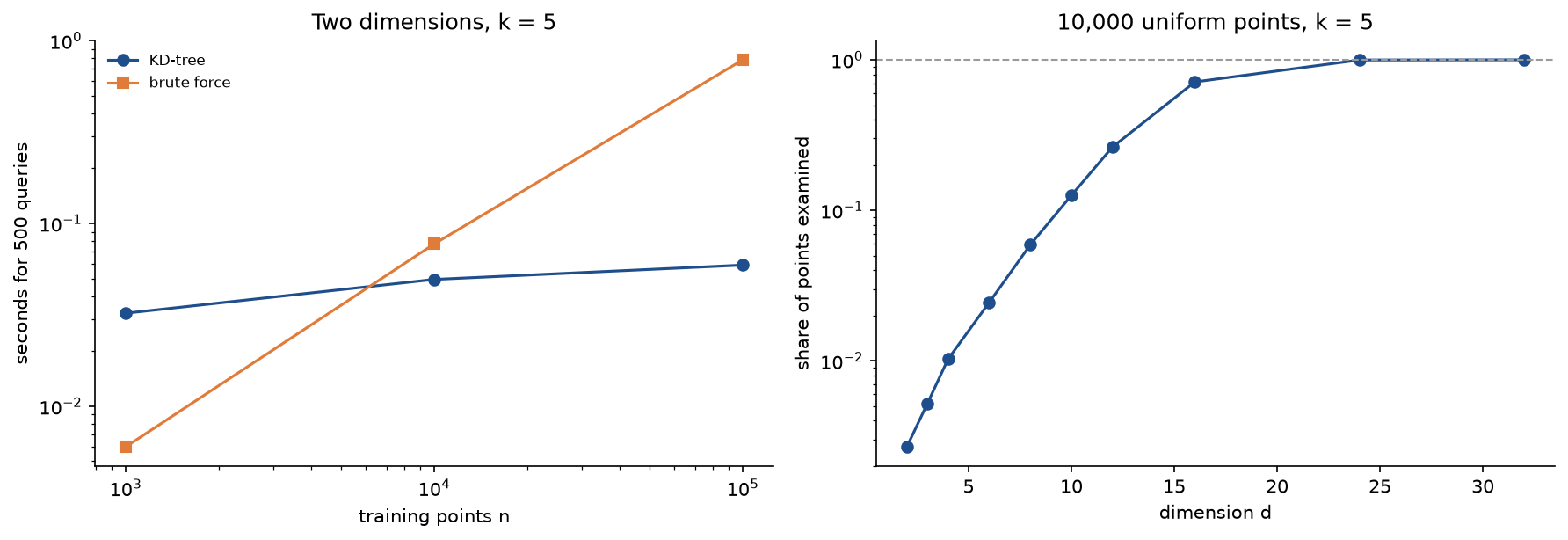
examples/high_dimensions.py times our tree for 500 queries with k = 5. In two dimensions it computes a few dozen distances per query, 34.6 for 1,000 points, 26.2 for 10,000 and 32.1 for 100,000, while brute force computes all n. In pure Python every visited node costs a few microseconds of interpreter overhead, so our tree loses at 1,000 points and is more than ten times faster than brute force at 100,000. With 10,000 points and growing dimension, the share of points the tree examines rises from 0.0027 in two dimensions to 0.0590 in eight, 0.7129 in sixteen and essentially all of them from 24 on; from three dimensions on, our tree is slower than brute force at this size. The timings themselves vary from run to run; the counts do not.

The 1-NN error bound

How good can a rule this simple be? Take two classes. The Bayes classifier predicts class 1 where η(x) > 1/2; at x it errs with probability m(x), the smaller of η(x) and 1 - η(x), and its error rate is the mean of m:

Now let the training set grow without limit. The nearest neighbour of a query x then lies arbitrarily close to x, so, for a smooth η, its label behaves like a fresh draw from the same distribution at x: class 1 with probability η(x), independently of the query's own label. The 1-NN rule predicts the neighbour's label and errs exactly when the two labels differ:

Averaging over x gives the asymptotic 1-NN error R₁. Since the mean of m² is at least the square of the mean of m, and since 2m(1 - m) ≥ m whenever m ≤ 1/2:

This is the bound of Cover and Hart (1967). In plain terms: with unlimited data, a rule that only ever looks at one neighbour makes at most twice as many errors as the best possible rule, whatever the distribution. The upper bound is attained when η is constant. Letting k grow too, slowly enough that k/n tends to zero, removes the factor: the k-NN error then converges to R* for every distribution (Stone, 1977). Neither statement says how much data is needed, and in high dimension the answer can be astronomically large.

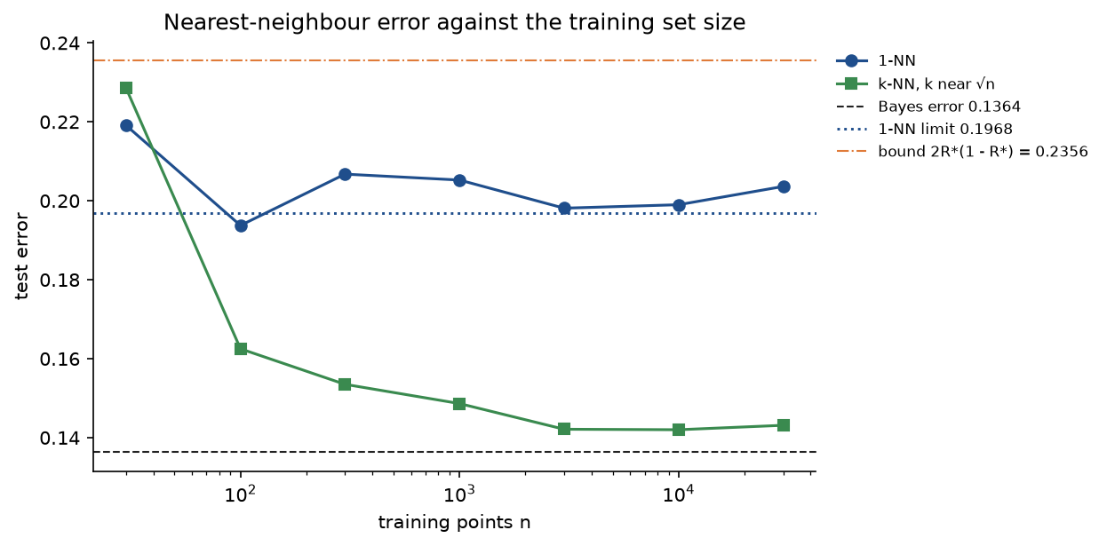
examples/error_bound.py measures both statements on the mixture. The asymptotic 1-NN error is 0.1968 and the Cover and Hart bound 0.2356, against R* = 0.1364. With growing training sets the 1-NN test error settles around its limit, 0.1981 at 3,000 points and 0.2036 at 30,000, while k near √n stays within 0.007 of the Bayes error from 3,000 points on: 0.1421 at 3,000 and 0.1431 at 30,000.

Worked example

Eight bean pods of two varieties, A and B, are measured by length in centimetres and mass in grams, and a new pod q of length 4.0 and mass 3.0 is to be classified:

• P1: length 5.0, mass 4.0, variety B.
• P2: length 2.0, mass 3.0, variety A.
• P3: length 5.5, mass 1.5, variety B.
• P4: length 4.0, mass 0.5, variety A.
• P5: length 5.9, mass 4.9, variety B.
• P6: length 1.0, mass 5.0, variety A.
• P7: length 2.5, mass 6.0, variety A.
• P8: length 8.0, mass 6.0, variety B.

All values are computed in double precision and shown to four decimals; sums written out from rounded terms can differ from them in the last digit.

Distances to the query

Each pod's offset from the query is its length and mass minus (4.0, 3.0). The five distances, in the order Euclidean, Manhattan, Minkowski with p = 3, Chebyshev and cosine, are:

• P1, offset (1.0, 1.0): 1.4142, 2.0, 1.2599, 1.0 and 0.0005.
• P2, offset (-2.0, 0.0): 2.0000, 2.0, 2.0000, 2.0 and 0.0570.
• P3, offset (1.5, -1.5): 2.1213, 3.0, 1.8899, 1.5 and 0.0703.
• P4, offset (0.0, -2.5): 2.5000, 2.5, 2.5000, 2.5 and 0.1318.
• P5, offset (1.9, 1.9): 2.6870, 3.8, 2.3938, 1.9 and 0.0012.
• P6, offset (-3.0, 2.0): 3.6056, 5.0, 3.2711, 3.0 and 0.2548.
• P7, offset (-1.5, 3.0): 3.3541, 4.5, 3.1201, 3.0 and 0.1385.
• P8, offset (4.0, 3.0): 5.0000, 7.0, 4.4979, 4.0 and 0.0000.

For P3, the Euclidean distance is √(1.5² + 1.5²) = √4.5 = 2.1213, the Manhattan distance 1.5 + 1.5 = 3, the Minkowski distance (1.5³ + 1.5³)^(1/3) = 6.75^(1/3) = 1.8899 and the Chebyshev distance the larger of 1.5 and 1.5, which is 1.5. For P2, the cosine similarity is (4.0 × 2.0 + 3.0 × 3.0) / (√(4² + 3²) × √(2² + 3²)) = 17 / (5 × 3.6056) = 0.9430, so the cosine distance is 0.0570. P8 is exactly twice the query, so it lies on the ray from the origin through the query and its cosine distance is zero, although it is the farthest pod by every other measure.

The vote with k = 3

• Euclidean: the three nearest are P1, P2 and P3, votes A 1 to B 2, prediction B.
• Manhattan: P1, P2 and P4, votes 2 to 1, prediction A.
• Minkowski with p = 3: P1, P3 and P2, votes 1 to 2, prediction B.
• Chebyshev: P1, P3 and P5, votes 0 to 3, prediction B.
• Cosine: P8, P1 and P5, votes 0 to 3, prediction B.

Manhattan distance prefers P4, whose offset lies along one axis (2.5), to P3, whose offset is diagonal (3.0), and the prediction flips to A. Chebyshev distance does the opposite: it ranks the diagonal P5 (1.9) ahead of P2 (2.0, all of it along one axis). The Euclidean and p = 3 distances sit between the two and agree here.

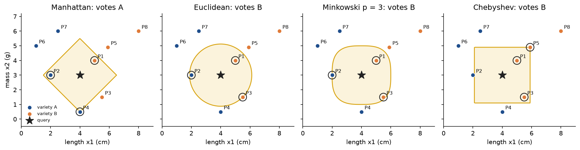
Each panel shows the smallest ball around the query that holds three pods. The balls have the shapes of the unit balls, which is the whole difference between the distances: the diamond reaches far along the axes and so catches P4, the square reaches far along the diagonals and so catches P5.

Even k, ties and distance weighting

With k = 4 under Euclidean distance the neighbours are P1 (B), P2 (A), P3 (B) and P4 (A): two votes each. Sending the tie to the smallest label answers A, which is what scikit-learn's KNeighborsClassifier does; sending it to the class of the nearest neighbour, P1, answers B. Distance weighting decides without a tie rule:

• A: 1/2.0000 + 1/2.5000 = 0.5000 + 0.4000 = 0.9000.
• B: 1/1.4142 + 1/2.1213 = 0.7071 + 0.4714 = 1.1785.

So the weighted prediction is B, with class shares 0.4330 for A and 0.5670 for B.

The Minkowski formula without the inner power

Written without the power inside the sum, the "Minkowski distance" of order 3 becomes the sum of the absolute offsets to the power 1/3: 2^(1/3) = 1.2599 for P1 and P2, 3^(1/3) = 1.4422 for P3 and 2.5^(1/3) = 1.3572 for P4. That is the Manhattan distance raised to the power 1/3, an increasing function of it, so it ranks the pods exactly as the Manhattan distance does and predicts A, while the correct p = 3 distance predicts B. For p = 2 and the offset (3, 4) the slip gives √7 = 2.6458 instead of 5.

Changing units and standardizing

Record the lengths in millimetres instead. The query becomes (40, 3.0), every length difference is ten times larger, and the Euclidean distances become 2.5000 for P4, √(10² + 1²) = 10.0499 for P1, √(15² + 1.5²) = 15.0748 for P3 and 15.2971 for P7. The nearest pod is now P4, the only pod with the query's length, whatever its mass, so the 1-NN prediction changes from B to A. The three nearest are P4, P1 and P3, still a majority for B, but the distance-weighted vote changes to A: 1/2.5 = 0.4000 against 1/10.0499 + 1/15.0748 = 0.0995 + 0.0663 = 0.1658. The pods did not change; only the bookkeeping did.

Standardize instead. The training means are (4.2375, 3.8625) and the standard deviations, dividing by n = 8, are (2.1696, 1.9091). The query becomes ((4.0 - 4.2375) / 2.1696, (3.0 - 3.8625) / 1.9091) = (-0.1095, -0.4518), and P1 becomes (0.3514, 0.0720), at distance √(0.4609² + 0.5238²) = √0.4868 = 0.6977. The standardized distances of P1 to P5 are 0.6977, 0.9218, 1.0466, 1.3095 and 1.3256, so the three nearest are P1, P2 and P3 and the prediction is B. Because standardized values do not depend on the units, exactly the same numbers come out of the millimetre version. Here the two standard deviations happen to be similar, so the standardized neighbours equal the centimetre ones.

A KD-tree by hand

Build a KD-tree with at most two pods per leaf. The root holds all eight pods; the length spreads from 1.0 to 8.0 and the mass from 0.5 to 6.0, so it splits on length. Sorted by length the pods are P6, P2, P7, P4, P1, P3, P5 and P8; the first four go left and the split value is the length of P1, 5.0. The left node's box is [1, 4] × [0.5, 6], wider in mass, so it splits on mass at 5.0 into the leaves {P4, P2} and {P6, P7}. The right node's box is [5, 8] × [1.5, 6], also wider in mass, so it splits on mass at 4.9 into {P3, P1} and {P5, P8}.

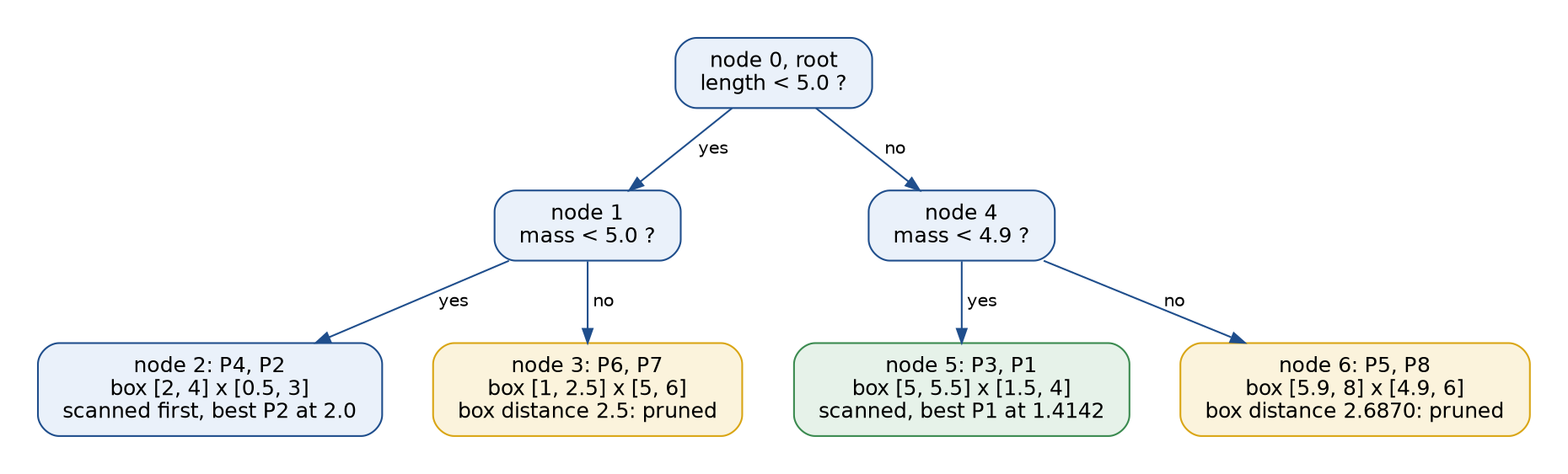
The diagram shows the tree with the outcome of the search below. The search for the single nearest pod to the query under Euclidean distance takes these steps:

1. Node 0, the root, box distance 0: descend. The query's length 4.0 is below 5.0, so node 1 comes first and node 4 later.
2. Node 1, box distance 0: descend. The mass 3.0 is below 5.0, so node 2 comes first and node 3 later.
3. Node 2, the leaf {P4, P2}, box distance 0: compute 2.5000 for P4 and 2.0000 for P2. Best so far P2 at 2.0000.
4. Node 3, the leaf {P6, P7}, box distance 2.5000: prune, since 2.5000 > 2.0000.
5. Node 4, box distance 1.0000: descend. The mass 3.0 is below 4.9, so node 5 comes first; node 6 has box distance 2.6870 > 2.0000 and is pruned at once.
6. Node 5, the leaf {P3, P1}, box distance 1.0000: compute 2.1213 for P3 and 1.4142 for P1. Best P1 at 1.4142.

The box distance of node 3 comes from the gaps 4.0 - 2.5 = 1.5 in length and 5.0 - 3.0 = 2.0 in mass, √(1.5² + 2²) = 2.5. Node 4's box starts at length 5.0, a gap of 1.0, with no gap in mass; node 6's gaps are 1.9 and 1.9, which gives 2.6870. The search returns P1, the same answer as the full list of distances, after computing four distances instead of eight. For k = 3 the search must first collect three candidates, so it also scans node 3; it then prunes node 6, whose box distance 2.6870 exceeds the third-best distance 2.1213, and computes six distances.

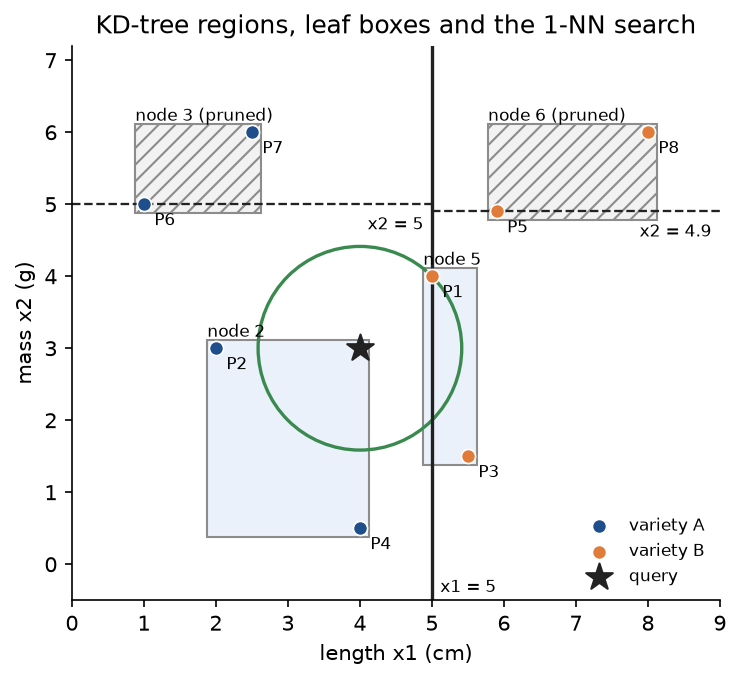
The final search ball, of radius 1.4142, touches neither pruned box, which is the geometric reason the pruning was safe. Every number in this section is asserted by tests/test_trace.py and tests/test_kd_build.py and printed by examples/worked_example.py.

The code

The package k_nearest_neighbors is plain NumPy, split into one module per idea. scikit-learn is imported only inside the functions of comparisons.py and digits.py, so the core works without it.

• arrays.py holds the Array types and as_points, which insists on one point per row.
• distances.py holds the distances between two vectors: Euclidean, Manhattan, Chebyshev, Minkowski and cosine, distance for any metric name, and minkowski_without_inner_power, the slip of the Pitfalls section.
• brute_force.py computes whole tables of distances in memory-bounded chunks with pairwise_distances and finds the k nearest per query with nearest_neighbors; smallest_k selects them in linear time and breaks ties by index.
• kd_tree.py holds the frozen KDTree, its nodes stored in flat arrays, with the exact search search, query and query_with_counts; kd_build.py builds it with build_kd_tree and traces a search with trace_kd_query.
• voting.py turns neighbours into predictions: vote_weights, class_scores, the two tie rules in resolve_ties, and votes_for_every_k, the running vote counts that give every k from one search.
• models.py holds KNNClassifier and KNNRegressor, frozen dataclasses whose fit returns a fitted copy; the classifier can search by brute force or with a KD-tree.
• scaling.py holds Standardizer and standardize_inside, which fits on training rows only.
• trace.py holds worked_example, trace_query, which keeps every distance and vote for one query, and the text renderings of a trace, a tree and a search.
• model_selection.py holds k-fold and stratified splits, holdout_errors, cross_validation_errors, training_errors and repeated_cross_validation, whose CrossValidationCurve knows its minimum and its one-standard-error choice.
• datasets.py generates the mixture with its exact class probabilities, the noisy sine, uniform cubes and noise features from seeds.
• theory.py computes the Bayes error, the 1-NN limit, the Cover and Hart bound, the exact bias and variance of k-NN regression and the concentration statistics.
• studies.py and dimension_studies.py run the measured studies behind the figures, and pitfalls.py the small measurements behind the Pitfalls section.
• digits.py loads the digits and cross-validates every candidate configuration for the sample project.
• comparisons.py builds the matching scikit-learn models and compares them with ours.
• plotting.py, study_plots.py and digit_plots.py draw every figure in the handbook's four colours.

Both search paths compare reduced distances, the Minkowski sum without its final root, which ranks points the same way, and take the root only for the k distances they return. The heart of the KD-tree is a depth-first search with an explicit stack. Without its tracing hook, the loop in KDTree.search reads:

while stack:
    node, bound = stack.pop()
    if bound > best[-1]:
        continue
    if self.is_leaf(node):
        values = self.leaf_reduced_distances(node, query, p)
        merged = np.concatenate([best, values])
        merged_index = np.concatenate([best_index, self.members(node)])
        keep = np.lexsort((merged_index, merged))[:k]
        best, best_index = merged[keep], merged_index[keep]
        continue
    near, far = self.children_in_visit_order(node, query)
    far_bound = self.box_reduced_distance(far, query, p)
    if far_bound <= best[-1]:
        stack.append((far, far_bound))
    stack.append((near, self.box_reduced_distance(near, query, p)))

The near child is pushed last so that it is popped first, and a node is skipped as soon as its box distance exceeds the current k-th best. Sorting the candidates by distance and then by training index makes the tree return exactly what brute force returns, ties included.

The examples and the project import the package, so install the repository first as described in the main README. Each example demonstrates one idea and runs in a few seconds from the repository root:

• examples/worked_example.py prints every value of the worked example in the order above and draws the neighbourhood balls and the KD-tree search.
• examples/choosing_k.py draws the decision regions for three k, compares training, cross-validation and test error, checks how stable the chosen k is over ten samples, and computes the bias-variance decomposition of k-NN regression.
• examples/error_bound.py measures the 1-NN and k-NN errors against the Cover and Hart bound for training sets from 30 to 30,000 points.
• examples/high_dimensions.py measures distance concentration, neighbourhood edges, the effect of noise features and the KD-tree against brute force by training set size and by dimension.
• examples/common_mistakes.py demonstrates each item of the Pitfalls section.
• examples/compare_with_sklearn.py compares the classifier, the regressor, the KD-tree and cross-validation with scikit-learn.

python machine-learning/k-nearest-neighbors/examples/worked_example.py
python machine-learning/k-nearest-neighbors/examples/choosing_k.py
python machine-learning/k-nearest-neighbors/examples/error_bound.py
python machine-learning/k-nearest-neighbors/examples/high_dimensions.py
python machine-learning/k-nearest-neighbors/examples/common_mistakes.py
python machine-learning/k-nearest-neighbors/examples/compare_with_sklearn.py

The sample project, project/digit_recognizer.py, applies everything to a realistic task: recognizing handwritten digits.

It splits the 1,797 images of 8 × 8 pixels by digit into 1,347 training and 450 test images and makes every choice by five-fold cross-validation on the training images alone: k from 1 to 15, Euclidean, Manhattan or cosine distance, uniform or distance-weighted votes, and raw or standardized pixels, twelve configurations in all. The lowest error wins; equal errors go to the smaller k and then to the configuration listed first. The test images are read once, after the choice. Options such as --seed, --test-fraction, --folds, --max-k, --metrics and --leaf-size change the setup, and --figures sends the two PNGs to another folder so a custom run does not overwrite the ones shown here; the default run takes a few seconds.

python machine-learning/k-nearest-neighbors/project/digit_recognizer.py
python machine-learning/k-nearest-neighbors/project/digit_recognizer.py --metrics manhattan cosine --max-k 25

The cross-validation errors of the best k per configuration are:

• Euclidean, uniform votes: raw pixels 0.0126 at k = 1, standardized 0.0304 at k = 1.
• Euclidean, distance weights: raw 0.0126 at k = 1, standardized 0.0267 at k = 3.
• Manhattan, uniform votes: raw 0.0163 at k = 1, standardized 0.0267 at k = 1.
• Manhattan, distance weights: raw 0.0163 at k = 1, standardized 0.0252 at k = 5.
• Cosine, uniform votes: raw 0.0141 at k = 1, standardized 0.0371 at k = 1.
• Cosine, distance weights: raw 0.0126 at k = 4, standardized 0.0371 at k = 1.

Three settings tie at 0.0126; preferring the smaller k and then the first listed, the choice is Euclidean distance on raw pixels with k = 1. It reads 443 of the 450 test images correctly, an accuracy of 0.9844.

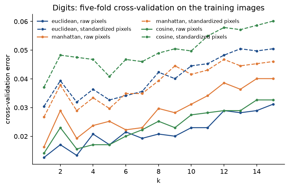
The curves show two effects at once. Standardizing hurts every distance, because it inflates nearly blank border pixels to the same weight as the strokes. And every curve jumps up at k = 2, where a split vote between two digits goes to the smaller one; the Euclidean error on raw pixels is 0.0126 at k = 1, 0.0171 at k = 2 and 0.0134 at k = 3.

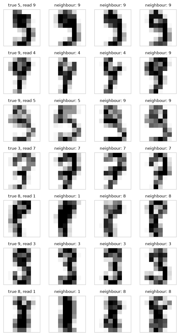
Each misread digit is written in a style closer to another digit's training examples than to its own. In three of the seven rows the second and third neighbours carry the true label, so k = 3 corrects them; it gets one other image wrong, and its test accuracy is 0.9889. A difference of two images out of 450 is noise, and cross-validation could not see it. The bundled data record no writer identity, so a random split may put digits of the same writer on both sides, and the test accuracy is probably a little optimistic for new writers. On these 64-dimensional images our KD-tree examines 46 % of the training images per query and is several times slower than brute force, 0.43 s against 0.09 s for the 450 test images in one run.

The notebook k_nearest_neighbors.ipynb is a guided tour in the order of this page: the worked example under five distances, the change of units, the KD-tree by hand, the choice of k on the mixture, the regression decomposition, ties, distance concentration, KD-tree timings, the 1-NN bound, the digits and the comparison with scikit-learn. The tests in tests check the worked example value by value, the mathematical properties above and the agreement with scikit-learn, and run in a few seconds:

python -m pytest machine-learning/k-nearest-neighbors

The synthetic sets are generated from fixed seeds by sample_mixture, noisy_sine and uniform_cube. The digits are the Optical Recognition of Handwritten Digits data of E. Alpaydin and C. Kaynak (1998) from the UCI Machine Learning Repository, available under the Creative Commons Attribution 4.0 licence. scikit-learn ships a copy of its test portion as sklearn.datasets.load_digits, so nothing is downloaded.

In practice

scikit-learn's KNeighborsClassifier, KNeighborsRegressor and KDTree do everything the package does, in compiled code. examples/compare_with_sklearn.py shows that they agree with ours:

• On 240 random points in three classes and 60 queries, KNNClassifier and KNeighborsClassifier(algorithm="brute") return the same neighbour indices and the same predictions for Euclidean, Manhattan, Chebyshev and Minkowski distance with p = 3, 1.5 and 0.5 and for cosine distance, with uniform and distance weights and k = 1, 4 and 9. Distances agree to within 4 × 10⁻¹⁵ and class shares to within 3 × 10⁻¹⁴. scikit-learn warns that p = 0.5 is not a metric and falls back to brute force.
• On the worked example scikit-learn answers A with shares (0.5, 0.5) for k = 4, and B with (0.433, 0.567) with distance weights.
• KNNRegressor matches KNeighborsRegressor exactly with uniform weights and to within 4 × 10⁻¹⁰ with distance weights. The small difference comes from scikit-learn computing Euclidean distances through the expansion of the square into dot products, which loses a few digits for close points.
• Our KDTree returns the same neighbours as sklearn.neighbors.KDTree on 100,000 points. The compiled tree builds about eight times faster and answers 500 queries about a hundred times faster, 0.0006 s against 0.06 s in one run.
• cross_validation_errors reproduces GridSearchCV fold for fold on the digits training images, and both choose k = 1.

The usual way to write the digits search in scikit-learn puts the scaler inside a pipeline, so it is refitted on every training fold:

from sklearn.model_selection import GridSearchCV
from sklearn.neighbors import KNeighborsClassifier
from sklearn.pipeline import make_pipeline
from sklearn.preprocessing import StandardScaler

pipeline = make_pipeline(StandardScaler(), KNeighborsClassifier())
grid = {
    "kneighborsclassifier__n_neighbors": list(range(1, 16)),
    "kneighborsclassifier__weights": ["uniform", "distance"],
}
search = GridSearchCV(pipeline, grid, cv=5).fit(features, labels)

Leave the scaler out when the features already share a meaningful unit, as the digits' pixels do. When to use which:

• Use the from-scratch version to learn the method, to trace a prediction by hand and to see where a KD-tree saves work.
• Use scikit-learn for anything else. algorithm="auto" chooses brute force, a KD-tree or a ball tree from the data size, the dimension and the metric; brute force with optimized linear algebra wins for high dimension or few queries, a tree for low dimension and many queries.
• Use k-NN as a baseline, for small to medium data sets with a meaningful distance, when predictions should be explained by pointing at similar cases, and when new labelled data must take effect without retraining.
• Scale features, and treat the scaling and the metric as hyperparameters to cross-validate, not as defaults.
• For text or embeddings, normalize rows to unit length and use Euclidean or cosine distance.
• For millions of high-dimensional vectors, use an approximate nearest-neighbour index such as FAISS, Annoy or an HNSW graph library. None of them is in this repository's dependency groups, so no agreement is tested here.
• When the data are high-dimensional with many irrelevant features, or the decision depends on a few features in a way a distance cannot express, prefer a model that learns which features matter, such as Decision trees, Ensembles or Logistic regression, or reduce the dimension first.

Pitfalls

examples/common_mistakes.py prints every number below.

• Features on different scales. A distance weighs each feature by its numeric range. Expressing the first mixture feature in units a hundred times smaller raises the test error at k = 25 from 0.1444 to 0.4796, because the distance then sees almost nothing else and that feature alone barely separates the classes; one extra noise column with a standard deviation of 100 raises it to 0.4958. Standardizing, fitted on the training rows, brings them back to 0.1452 and 0.1792. In the worked example a change from centimetres to millimetres alone flips the 1-NN prediction.
• Standardizing by reflex. When features share a unit and their spread is meaningful, standardizing hurts. On the digits, where 12 of the 64 pixels have a standard deviation below 0.5 and 3 are constant, it raises the 1-NN cross-validation error from 0.0126 to 0.0304, because nearly blank border pixels get the same weight as the strokes. Fit any scaler inside the cross-validation folds; Data leakage and pitfalls measures what happens otherwise.
• The Minkowski exponent in the wrong place. The power p belongs on every absolute difference inside the sum. Written outside the sum only, the formula is a monotone function of the Manhattan distance and always picks the Manhattan neighbours: on 200 random queries in four dimensions it chose exactly the Manhattan five nearest every time, a share of 1.0000, while the correct p = 3 distance chose them for one query in 200, a share of 0.0050. The slip is easy to make when the formula is written from memory, and nothing crashes.
• Judging k by the training error. At k = 1 the training error is 0 and the test error on the mixture is 0.1938. Use cross-validation, and do not trust its minimum blindly: on the mixture the minimum at k = 3 gives a test error of 0.1684, the one-standard-error choice k = 29 gives 0.1460.
• Even k with two classes. With k = 4, uniform votes tie on 0.1062 of the mixture test points and the tie rule decides them; k = 5 never ties. Distance weighting removes ties but makes the rule behave more like a smaller k: on the mixture its test error is 0.1704 at k = 4 and 0.1606 at k = 5, against 0.1618 and 0.1532 with uniform votes. The digits curves above show the same jump at k = 2.
• Ties at the k-th distance. Take four points at distance 1 from the origin, two per class, and query the origin: swapping two pairs of training rows changes the k = 1 prediction from 1 to 0 and the k = 3 prediction from 1 to 0. Our rule keeps the lower index; libraries make no promise, and scikit-learn's documentation warns that the result then depends on the order of the training data. Integer or rounded features make such ties common.
• Cosine distance for positions. The cosine ignores vector length, so the farthest pod of the worked example, P8, is the cosine nearest. On the mixture, cosine distance raises the test error at k = 25 from 0.1444 to 0.1988. Use it for directions, such as word counts or embeddings, not for coordinates measured from an arbitrary origin.
• Irrelevant features and high dimension. Every useless feature adds noise to every distance. On the mixture, ten noise features raise the test error from 0.1684 to 0.4180. Select features or reduce the dimension before relying on neighbours.
• Expecting an index to fix high dimension. A KD-tree is exact but examines almost every point once the dimension exceeds about 15 to 20 for uniform data, and is then slower than brute force: on the digits ours examines 46 % of the training set and loses to brute force.
• Forgetting the cost of laziness. Fitting is free, but every prediction scans the training set unless an index helps, and the whole training set must be kept and shipped with the model. For latency-bound applications, measure prediction time on the full data before choosing k-NN.

Further reading

• E. Fix and J. L. Hodges, "Discriminatory analysis. Nonparametric discrimination: consistency properties", Report 4, USAF School of Aviation Medicine, 1951; reprinted in International Statistical Review 57(3), 238-247, 1989. The origin of the nearest-neighbour rule.
• T. M. Cover and P. E. Hart, "Nearest neighbor pattern classification", IEEE Transactions on Information Theory 13(1), 21-27, 1967. The 1-NN error bound.
• C. J. Stone, "Consistent nonparametric regression", Annals of Statistics 5(4), 595-620, 1977. Universal consistency of k-NN when k grows and k/n tends to zero.
• J. L. Bentley, "Multidimensional binary search trees used for associative searching", Communications of the ACM 18(9), 509-517, 1975. The KD-tree.
• J. H. Friedman, J. L. Bentley and R. A. Finkel, "An algorithm for finding best matches in logarithmic expected time", ACM Transactions on Mathematical Software 3(3), 209-226, 1977.
• K. Beyer, J. Goldstein, R. Ramakrishnan and U. Shaft, "When is 'nearest neighbor' meaningful?", International Conference on Database Theory, 1999. Distance concentration.
• C. C. Aggarwal, A. Hinneburg and D. A. Keim, "On the surprising behavior of distance metrics in high dimensional space", International Conference on Database Theory, 2001. Why small p keeps more contrast in high dimension.
• T. Hastie, R. Tibshirani and J. Friedman, The Elements of Statistical Learning, second edition, Springer, 2009, sections 2.3, 2.5 and 7.10 and chapter 13.
• L. Devroye, L. Györfi and G. Lugosi, A Probabilistic Theory of Pattern Recognition, Springer, 1996, chapters 5 and 11.
• R. O. Duda, P. E. Hart and D. G. Stork, Pattern Classification, second edition, Wiley, 2001, chapter 4.
• Y. A. Malkov and D. A. Yashunin, "Efficient and robust approximate nearest neighbor search using hierarchical navigable small world graphs", IEEE Transactions on Pattern Analysis and Machine Intelligence 42(4), 824-836, 2020.
• E. Alpaydin and C. Kaynak, "Optical Recognition of Handwritten Digits", UCI Machine Learning Repository, 1998, https://archive.ics.uci.edu/ml/datasets/Optical+Recognition+of+Handwritten+Digits.
• scikit-learn user guide, "Nearest Neighbors".