The machine learning landscape

Machine learning replaces hand-written rules with rules estimated from examples. That one idea takes several forms, depending on what the examples contain: answers to imitate, raw inputs whose structure is to be found, answers manufactured from the data itself, or only rewards for the learner's own actions. All of them share one difficulty. A model is judged by how well it does on data it has not seen, yet it can only be fitted to data it has seen, and the more flexible it is, the better it fits the training data and the less that fit says about new data. This page maps the kinds of learning and the handbook topics that treat each one, lays out the modelling workflow from framing a problem to reporting a test score, and then studies the gap between fitting and predicting: it derives the bias-variance decomposition for squared error, works it by hand on four three-point training sets, measures it by simulating polynomial fits over a thousand resampled training sets, turns it into learning curves and validation curves, and uses them to choose a model in a complete study. It closes with the no-free-lunch argument checked by enumeration. Afterwards you will be able to place any method in this handbook on the map, run a modelling project in an order that keeps its evaluation honest, and diagnose from a pair of curves whether a model needs more data, more capacity or neither.

To run the code in this topic, install the base group, and the ml group for the comparisons with scikit-learn.

Intuition

Suppose a pump carries a vibration sensor and someone must decide, every minute, whether the pump is about to fail. The traditional approach is to ask an engineer for rules: if the vibration amplitude exceeds a threshold and the temperature has risen for ten minutes, raise an alarm. The rules are explicit, and they are only as good as the engineer's understanding, which for a complicated machine is incomplete. The learning approach collects a year of sensor readings together with the record of which minutes preceded a failure, and lets an algorithm find the function from readings to "failure soon" that best reproduces that record. The engineer's knowledge does not disappear. It moves into the choice of inputs, the family of functions the algorithm may consider and the way errors are counted.

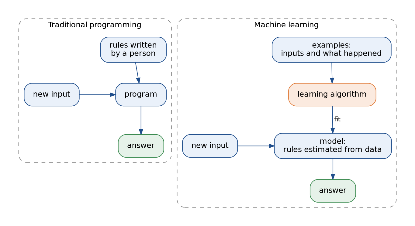
In both panels a new input ends as an answer. What differs is where the rules come from: written by a person on the left, fitted to examples on the right.

A standard definition (Mitchell, 1997) makes the idea testable: a program learns from experience E with respect to a task T and a performance measure P if its performance at T, as measured by P, improves with E. For the pump, T is predicting failures, E is the year of labelled readings and P might be the fraction of failures caught at a fixed false-alarm rate. The definition says nothing about how the program improves, only that the improvement can be measured, and the measuring is where most of the craft lies.

Learning pays when the rules are unknown or too many to write down (recognising a face, transcribing speech), when they change (spam, fraud), or when they differ between users (recommendations). It is the wrong tool when the rules are known and stable (computing a tax), when there are too few examples to estimate anything, or when every decision must be justified by a rule a person can audit.

The kinds of learning

The kind of learning is decided by what the examples contain. In supervised learning every input comes with the answer the model should produce. In unsupervised learning there are inputs only, and the goal is to describe their structure. Self-supervised learning is supervised learning on answers cut out of the data itself, which is how language models are trained on raw text. Reinforcement learning has no answers at all: the learner acts, the environment responds with rewards, and the learner must work out which of its actions earned them. Each kind below is given with what its examples contain, what the model produces, one example, and the topics that treat it.

• Supervised regression. Inputs with numeric targets; the model produces a number for each input, for example tomorrow's electricity demand from the weather forecast. Treated in Linear regression, k-nearest neighbours, Decision trees, Ensembles and Perceptrons and multilayer networks.
• Supervised classification. Inputs with categorical labels; the model produces a label, or a probability for each label, for example whether an email is spam. Treated in Logistic regression, Naive Bayes, k-nearest neighbours, Decision trees, Support vector machines, Text classification and Convolutional networks.
• Clustering. Inputs only; the model produces a group for each input, for example customer segments from purchase histories. Treated in Clustering.
• Dimensionality reduction. Inputs only; the model produces a few numbers that summarise many, for example 64 sensor channels compressed to 3 for plotting and monitoring. Treated in Dimensionality reduction.
• Density estimation. Inputs only; the model says how probable each input is, for example which word sequences are likely in a language. Treated in Probability and statistics and N-gram language models.
• Anomaly detection. Inputs, mostly normal ones; the model produces a score of how unusual an input is, for example a card payment unlike the holder's history. Treated in Anomaly detection, Edge anomaly detection and Intrusion detection.
• Pattern mining. Sets of items; the model produces frequent combinations and rules between them, for example products often bought together. Treated in Frequent pattern mining and Recommender systems.
• Self-supervised learning. Raw data whose targets are parts of itself; the model produces a representation, or fills in missing parts, for example the next word of a sentence from the words before it. Treated in Text representations, A tiny GPT and Transfer learning.
• Reinforcement learning. States, actions and rewards from the learner's own experience; the model produces a policy, which action to take in each state, for example balancing a pole on a cart from a reward for every step it stays up. Treated in Markov decision processes, Q-learning, Deep Q-networks and Game-playing agents.

The boundaries are not walls. Anomaly detection becomes classification once enough anomalies are labelled. Semi-supervised learning combines a few labelled examples with many unlabelled ones. Link analysis (PageRank) and recommendation learn from the structure of a graph or a ratings matrix rather than from labelled rows. A self-supervised model is usually only a first stage: its representation is then fine-tuned with labels for a supervised task, the subject of Transfer learning.

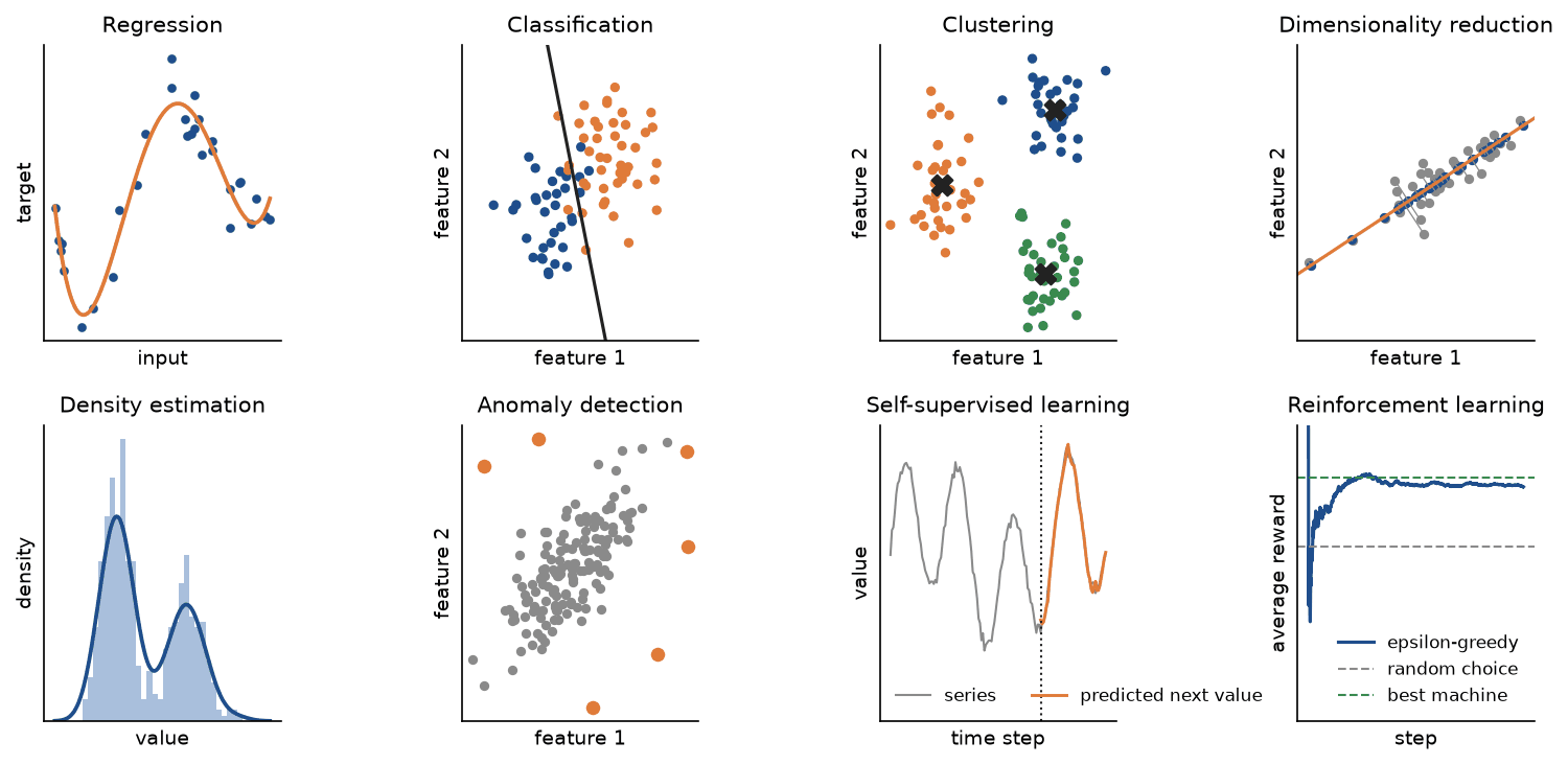
Each panel is one small synthetic problem solved from scratch by examples/kinds_of_learning.py. The regression fits a degree-4 polynomial (training error 0.0533). The classifier is a logistic regression fitted by Newton's method and labels 88.75 % of its 80 training points correctly. k-means splits 105 points into clusters of 34, 35 and 36. The first principal direction keeps 95.07 % of the variance of a stretched cloud. A Gaussian kernel density estimate traces the two bumps of a 500-value sample. The squared Mahalanobis distance flags 6 of 155 readings, among them all 5 planted outliers. The self-supervised panel predicts each value of a series from the four before it, training only on targets cut from the series itself, and misses the last 46 values by 0.0738 (root mean square). The reinforcement panel is an epsilon-greedy player of three slot machines with unknown payout rates 0.3, 0.5 and 0.7; its average reward over the last 500 of 1500 plays is 0.6700, between random play (0.5) and always playing the best machine (0.7).

Kinds of data

The same functions (predict, group, compress, score, mine) recur across very different data, and the type of data usually decides the representation before the learning method is chosen.

• Tables of measurements, one row per case and one column per feature: most of this part, and The analytics workflow.
• Time series and sensor streams, as windows of recent values or summary statistics: Activity recognition and Edge anomaly detection.
• Text, as tokens, counts or embeddings: Text processing and Text representations.
• Images and video, as arrays of pixels or learned convolutional features: Digital images and colour and Convolutional networks.
• Audio, as spectrograms or frame features: Audio features.
• Graphs and links, as adjacency matrices or random walks: PageRank.
• Transactions, as sets of items: Frequent pattern mining.

The modelling workflow

Whatever the kind of learning, a project that ends in a trustworthy number follows roughly the same loop. The order matters more than any single step: the test set is split off before anything is learned from the data, and it is used once, at the end.

The two dashed loops are where the work goes: most projects go round the inner loop many times before the test set is touched, and the outer loop starts again when the world the model serves has changed.

1. Frame the problem. State what is predicted, from which inputs and at what moment, so that only information available at that moment is used. Choose a metric that matches the cost of the errors that matter: a fraud detector that misses fraud and one that blocks honest customers fail differently. Evaluation metrics covers the choice.
2. Split the data. Set the test set aside before looking at the data in detail, and split by whatever will be new when the model is used: new patients, new days, new devices. Splitting rows at random when the rows come in groups or in time order is the most common way to get a score that does not survive deployment; Data leakage and pitfalls demonstrates many variants.
3. Measure a baseline: the mean of the training targets for regression, the most frequent class for classification, yesterday's value for a forecast, or the existing hand-written rule. A model is interesting only by how much it beats this, and a model that does not beat it is broken, not modest.
4. Train candidate models on the training data only, including every preprocessing step that learns from data, such as scaling or feature selection.
5. Validate. Choose the capacity (degree, depth, number of neighbours, regularization strength) and other settings with a validation set or cross-validation on the training data, never with the test set.
6. Analyse the errors. Look at the worst predictions and at the error by slice, and use learning curves to decide whether more data, more capacity or better inputs would help. Then go back to step 4.
7. Test once. Score the chosen model on the untouched test set and report the result with its uncertainty. A second look at the test set after a change turns it into a validation set.
8. Deploy and monitor. Inputs drift after deployment, and a model that was right last year can quietly stop being right. Honest evaluation covers reporting.

Underfitting and overfitting

The quantity a project cares about is the error on new data from the situation the model will be used in, the generalization error. The training error is a poor guide to it for a reason that is easy to state: a flexible model can make its training error small by bending towards the noise in the particular examples it saw, and noise does not repeat. Two failure modes bracket the right amount of flexibility. A model too rigid to follow the real pattern underfits: it is wrong in the same way on every training set and on new data, and the error it makes is called bias. A model so flexible that it follows the noise overfits: its fit changes a lot from one training set to the next, and that instability is called variance. The bias-variance decomposition below makes both words precise for squared error, and the worked example shows them on numbers small enough to check by hand.

How the topics connect

The map groups the parts of this handbook by the kind of learning they serve. Arrows point from a group to the groups that build on it.

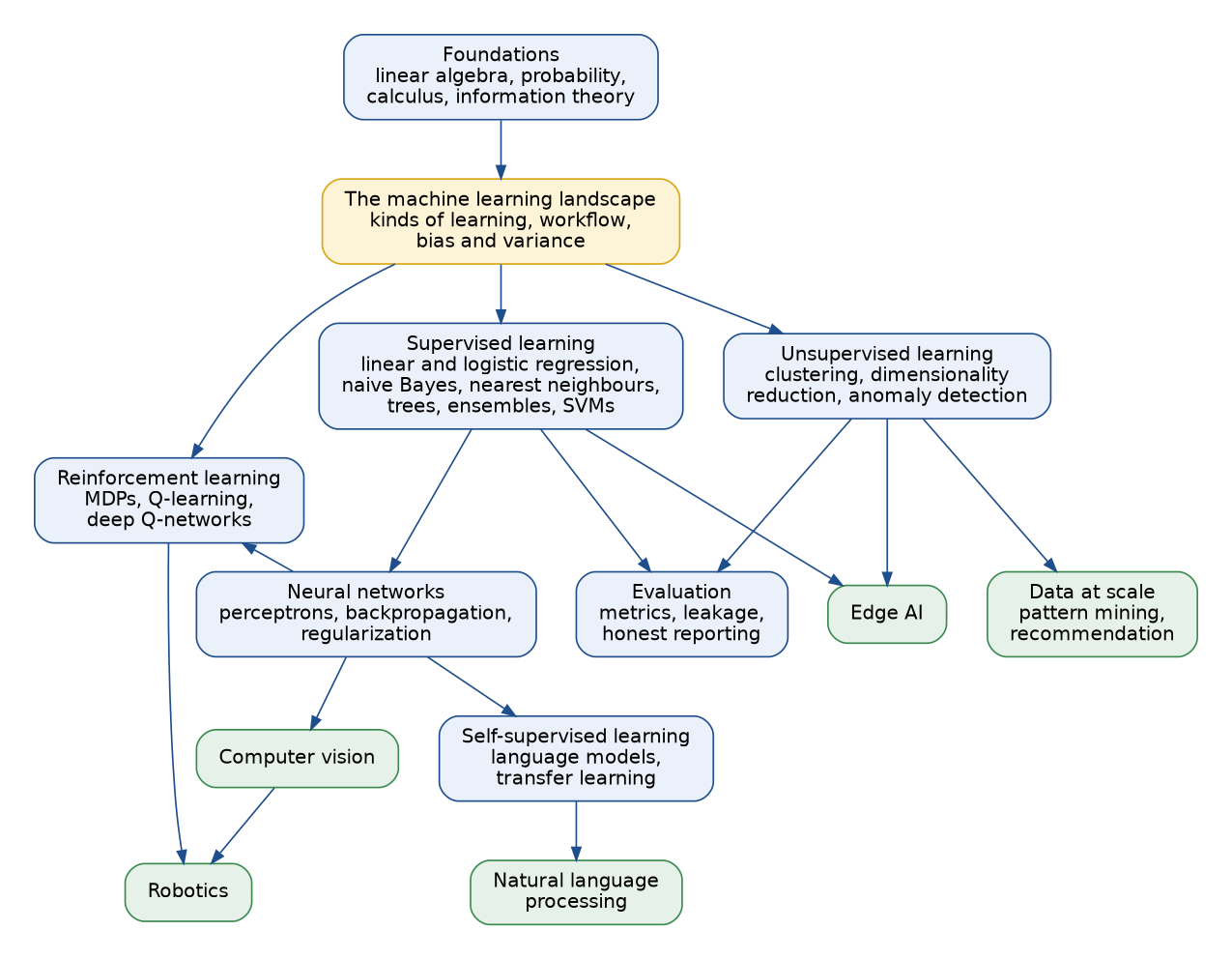
Within the groups the order is just as deliberate. Calculus and optimization lead to linear regression, which leads to logistic regression and from there to perceptrons, backpropagation and regularization. Probability leads to naive Bayes, information theory to decision trees and then ensembles, and linear algebra to dimensionality reduction. Markov decision processes lead to Q-learning, which meets neural networks in deep Q-networks, and n-gram language models lead to a tiny GPT and then to transfer learning.

How it works

Notation

An input is x and its target y; for regression y is a real number. Pairs (x, y) are drawn from an unknown distribution P, and a training set D holds n of them. A loss L(y, ŷ) is the cost of predicting ŷ when the truth is y; on this page it is mostly the squared error. The hypothesis class F is the family of functions the learner may choose from, and the learned function, written f̂ with the subscript D in the formulas, is the member of F it returns when trained on D. The regression function f(x) is the average target at x, the best possible predictor under squared loss, and the noise ε = y - f(x) has mean zero and variance σ². The average prediction at x over all training sets, written with a bar, is f̄(x).

In the formula images a hat marks a quantity estimated from data, a bar an average over training sets, and the subscript D a dependence on the training set. In the text the same quantities are named in words, and indexed quantities are written plainly, so x0 is the query point and y1, y2 and y3 are the three targets of a training set.

Learning as risk minimization

The goal is a function with small expected loss on a new pair drawn from the same distribution, its risk:

P is unknown, so the learner minimizes the average loss on the training set instead, the empirical risk, over a chosen family of functions:

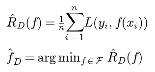
This is empirical risk minimization. Linear regression is the case where F holds the linear functions and the loss is squared; a neural network is a much larger F; k-nearest neighbours and decision trees fit the same mould with less obvious families.

For squared loss the best possible predictor can be found exactly. At a fixed x, write m(x) for the average target at x and add and subtract it inside the loss of any constant prediction c:

The middle expectation is zero, so the loss is smallest at c = m(x). The best predictor is therefore the regression function, and even it suffers the Bayes risk, the average variance of y at fixed x, which is σ² when the noise has constant variance. No model, however clever, beats that floor on average.

The excess risk of the learned function splits into two parts by adding and subtracting the risk of the best member of the class, written with the subscript F:

A richer class lowers the approximation error, because it contains functions closer to f, and usually raises the estimation error, because the training set picks among more candidates and is fooled more easily. Bias and variance are the squared-error versions of the same tension.

Polynomial regression as a capacity dial

Fitting a polynomial of degree d by least squares is linear regression on the features 1, x, x², up to x to the power d, so it has p = d + 1 coefficients. The feature matrix Φ has one row per training input:

The degree is a single number that controls capacity, which makes polynomials the standard laboratory for generalization. Two facts follow from the nesting of the classes, since every polynomial of degree d is also one of degree d + 1 with a zero leading coefficient:

• The minimum training error can only fall or stay the same as the degree grows. A fit at a higher degree that has a larger training error than one at a lower degree is a numerical failure, not a property of the data (see Pitfalls).
• With n distinct inputs and p = d + 1 ≥ n coefficients, some polynomial passes through every training point and the training error is zero, whatever the noise. The training error then says nothing at all about the test error.

The fitted values at the training inputs are a fixed matrix times the targets. That matrix, the hat matrix H, projects onto the column space of Φ, and its trace counts the coefficients:

The trace step uses tr(AB) = tr(BA), which moves the first Φ to the end. Linear regression treats the solution of the normal equations, gradient descent and ridge regularization, a continuous capacity dial in place of the integer degree.

Training, validation and test error

The training error, the empirical risk of the learned function on its own training set, is a biased estimate of its risk: the same data chose the function and scored it. A test set of m pairs drawn independently of D gives an unbiased estimate, whose standard error is the standard deviation s of the m losses divided by the square root of m:

The estimate is unbiased only as long as nothing about the model was decided by looking at those m pairs. When the same held-out data is used to choose among K candidates, the score of the winner is the minimum of K noisy estimates, and the expected minimum is never larger than the smallest expected value:

The reported score is optimistic. That is why choices are made on a validation set or by cross-validation, and the test set is kept for one final measurement. Data leakage and pitfalls derives the size of this optimism, and Evaluation metrics treats cross-validation and its variants.

Why the training error is optimistic

For least squares the optimism can be computed exactly. Fix the training inputs, so that only the noise is random, and write the bold f for the vector of true values at the training inputs and ε for the noise vector, whose entries have mean zero, variance σ² and no correlation. The residuals split into a part from the true function and a part from the noise. The cross term between them has mean zero, and for any fixed matrix A the expected value of ε transposed times A times ε is σ² times the trace of A. Since I - H is symmetric and idempotent too, its square is itself:

Now draw fresh targets y′ at the same inputs, with noise independent of the first. The old fit misses them by the same systematic part, plus the new noise, plus the old noise it copied into its fit, which contributes σ² times the trace of H transposed H, that is p σ²:

Dividing by n and writing B for the squared bias averaged over the training inputs gives both expected errors:

Apart from what it does to the bias, each parameter lowers the expected training error by σ²/n and raises the expected error on new data by the same amount, so the optimism is exact:

Adding that amount to the training error is Mallows' Cp, an early model-selection rule; the Akaike information criterion has the same form. The derivation also shows where the variance goes: averaged over the training inputs it is σ² p / n, growing linearly with the number of parameters.

The bias-variance decomposition

Let the training set D be random, with inputs and noise both drawn afresh each time, and let a new observation at a fixed input x0 be y0 = f(x0) + ε0, where ε0 has mean zero and variance σ² and is independent of D. The expected squared error of the learned function at x0 averages over training sets and over the new noise.

Step 1 separates the noise. Write the error as the new noise plus the gap between the truth and the fit, and expand the square:

The first term is σ². The middle term factorizes because ε0 is independent of D, and the mean of ε0 is zero, so it vanishes.

Step 2 separates the bias. Add and subtract the average prediction f̄(x0) in the last term:

The first factor of the middle term is a constant, and the expectation it multiplies is zero by the definition of the average prediction. What remains is the decomposition:

• The noise is the part of y0 that no function of x0 can predict. It does not depend on the learner and does not shrink with more data.
• The bias is how far the average fit lies from the truth: a systematic error that would remain if the learner could be trained on infinitely many training sets and its fits averaged.
• The variance is how much the fit moves when the training set changes: the price of letting the data decide.

Averaging over x0 drawn from the input distribution gives the same decomposition of the expected test error, with integrated bias squared and integrated variance. The derivation used nothing about the learner, so it holds for any method under squared loss; for other losses there is no comparably clean additive split (see Pitfalls).

For a linear smoother, a learner whose prediction is a fixed weighted sum of the training targets with weights w(x0) that depend on the inputs only, both terms have closed forms when the inputs are fixed:

Least squares on polynomial features is a linear smoother, and its weight vector at a new input is the corresponding row of the hat matrix. Two consequences are used in the worked example: the bias and variance depend on the noise only through its mean and covariance, and the weights sum to one whenever the features include a constant, because the fit must reproduce a constant target exactly.

Measuring bias and variance by simulation

The closed forms need fixed inputs. When the inputs change from one training set to the next, bias and variance are measured by brute force: draw many training sets, fit every degree to each, keep every prediction on a grid of query points, and compare the average fit with the truth and the individual fits with their average. The realistic simulation uses the true function f(x) = sin(4x + 1) + x/2 on the interval from -1 to 1, training sets of n = 20 points with Gaussian noise of standard deviation σ = 0.4, so the noise floor is σ² = 0.16, and stratified inputs: one input drawn uniformly inside each of 20 equal bins, so every set covers the interval. One thousand training sets are drawn; on each, polynomials of degree 0 to 12 are fitted and evaluated at 201 evenly spaced query points, where a fresh noisy target is drawn too, so the test error can be measured directly as well.

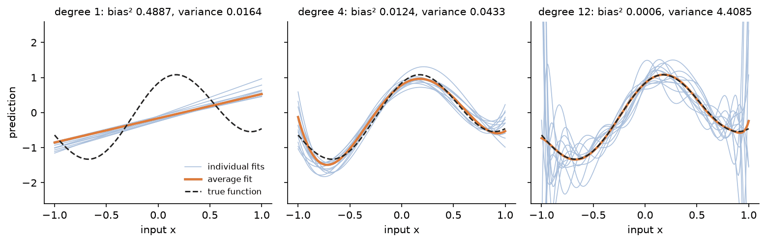
The panels show the two failure modes. The lines are nearly identical to each other and all wrong in the same way, which is bias; the degree-12 curves are right on average and far from each other, which is variance.

For each degree, examples/bias_variance_simulation.py prints bias squared, variance, their sum plus the noise, the simulated test error and the training error:

• Degree 0: 0.6440, 0.0078, 0.8119, 0.8148 and 0.8011.
• Degree 2: 0.2223, 0.0271, 0.4094, 0.4101 and 0.3507.
• Degree 4: 0.0124, 0.0433, 0.2157, 0.2170 and 0.1292.
• Degree 5: 0.0034, 0.0548, 0.2183, 0.2192 and 0.1131.
• Degree 6: 0.0003, 0.0698, 0.2300, 0.2308 and 0.1033.
• Degree 8: 0.0001, 0.1531, 0.3131, 0.3132 and 0.0872.
• Degree 10: 0.0008, 0.5819, 0.7427, 0.7441 and 0.0711.
• Degree 12: 0.0006, 4.4085, 4.5691, 4.5728 and 0.0549.

The decomposition predicts the measured test error to within 0.6 % at every degree. Bias squared falls by four orders of magnitude between degrees 0 and 7, variance grows more than 500-fold between degrees 0 and 12, and the expected error is smallest at degree 4, with degree 5 a close second. The training error falls at every degree and from degree 4 on lies below the noise floor, which no predictor can beat on new data. The small rise of bias squared beyond degree 9 is simulation noise: the average of 1000 fits is itself uncertain, and on average this plug-in estimate of bias squared exceeds the true value by the variance divided by the number of training sets, about 0.0044 at degree 12.

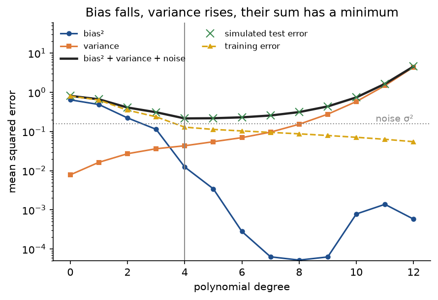
The crosses of the simulated test error sit on the black curve of the decomposition, which is the decomposition confirmed by measurement. The gap between the black curve and the dashed training error is the optimism, and it widens with the degree.

With fixed rather than stratified inputs the simulation can be checked against the closed forms. With the 20 inputs on an even grid and 4000 training sets, the simulated bias squared and variance are 0.4909 and 0.0154 at degree 1 against the exact 0.4909 and 0.0153, 0.0136 and 0.0356 at degree 4 against 0.0136 and 0.0352, and 0.0000 and 0.0880 at degree 10 against 0.0000 and 0.0871.

Learning curves and validation curves

A learning curve plots training error and validation error against the number of training examples for a fixed model. A validation curve plots both against a capacity setting, such as the degree, for a fixed amount of data. The formulas of the optimism section predict their shapes:

As n grows the training error rises (each example is harder to memorize), the validation error falls (the fit stabilizes), and both approach the error of the best function in the class, σ² plus the approximation error, which B settles to. The gap closes at the rate p/n, and the level the curves close towards is set by the bias. For a fixed n, as capacity grows the training error falls steadily, while the validation error falls while bias dominates and rises once variance does. The curves therefore support three diagnoses:

• Training and validation error close together, both well above the noise level: high bias, underfitting. More capacity, better features or less regularization help; more data will not.
• Training error low, validation error much higher, the gap shrinking as n grows: high variance, overfitting. More data, less capacity, regularization or averaging many models help.
• Both curves meeting near the noise floor: the model is limited by the information in the inputs. New inputs that carry more information help, not a different model.

examples/learning_and_validation_curves.py computes learning curves for degrees 1, 4 and 10 by five-fold cross-validation on 1000 points of the same problem, with 15 to 800 training examples.

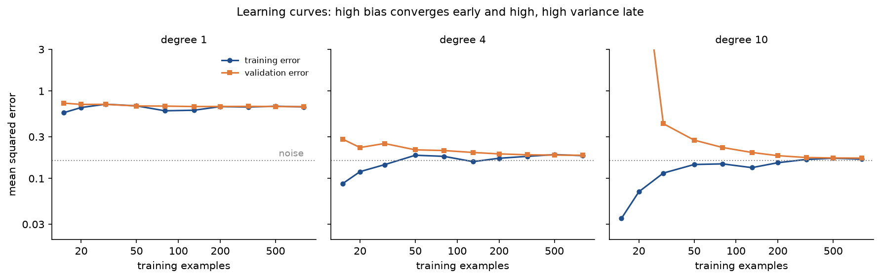
The three panels show the three diagnoses. Degree 1 has converged by about 50 examples with both errors near 0.66, four times the noise level: high bias, and more data cannot help. Degree 10 has a validation error of 6365 at 15 examples and 70.49 at 20, and is still improving at 800, where it reaches 0.1712: high variance. Degree 4 starts at 0.2823 and reaches 0.1845 at 800 examples.

The best degree depends on the amount of data, and a validation curve computed on a single data set is noisy. Over 30 independent data sets of 40 points each, the median five-fold validation curve is lowest at degree 4, but the degree chosen on individual data sets ranges from 4 to 11. With 400 points the median curve is lowest at degree 6, and beyond degree 6 the curve is nearly flat, because each extra parameter now costs only about σ²/n of variance; the chosen degree still ranges from 5 to 13.

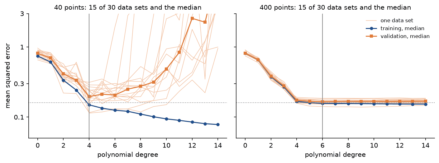
The chosen degree matters much less than its spread suggests when the curve is flat near its minimum, as with 400 points, and much more when it is not, as with 40.

Choosing the capacity: cross-validation and the one-standard-error rule

k-fold cross-validation reuses the training data for validation. It splits the rows into k folds, trains on k - 1 of them, scores the remaining one, and repeats until every fold has been scored once. For each degree d the cross-validated error is the average of the k fold scores, and its standard error is their standard deviation divided by the square root of k:

The estimate refers to models trained on (k - 1)/k of the rows, slightly fewer than the final model will see, so it is a little pessimistic. Picking the degree with the lowest cross-validated error is the obvious rule. The one-standard-error rule prefers simplicity: it takes the smallest degree whose error lies within one standard error of the minimum, on the grounds that differences smaller than the noise in the estimate are not evidence:

The sample project applies both rules inside the whole workflow. The test rows are set aside first, every choice is made by cross-validation on the remaining development rows, and the test rows are scored once at the end:

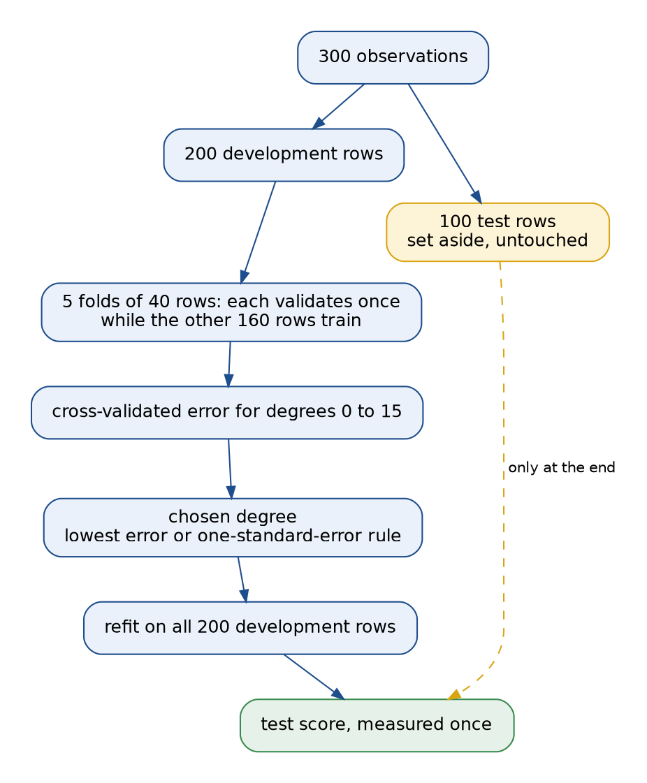
The dashed arrow is the whole discipline: the test rows enter the computation in exactly one place, after the degree is fixed.

No free lunch

Every learner generalizes by assuming something about the examples it has not seen. A nearest-neighbour classifier assumes that nearby inputs share labels; a low-degree polynomial assumes the target is smooth; a convolutional network assumes that a pattern means the same thing wherever it appears in an image. The no-free-lunch theorem (Wolpert, 1996) says that without such an assumption nothing can be learned: averaged uniformly over every possible target function, all learning algorithms have the same expected error on inputs outside the training set.

The argument is short for a finite input space and binary labels. A target is any function t from the inputs to the labels 0 and 1, so there are 2 to the power of the number of inputs of them. Fix a training set S of inputs and take any deterministic learner; its prediction h at an unseen input x depends only on S and the training labels of t. Group the targets by their values on S. Within a group, exactly half of the targets give x the label 0 and half the label 1, while the prediction at x is the same for the whole group. So the learner is right at x on exactly half of every group, and therefore on exactly half of all targets:

This holds for every unseen input and every learner, and averaging over the unseen inputs gives an off-training-set accuracy of exactly one half, the same as guessing. examples/no_free_lunch.py checks it on the eight 3-bit inputs, training on the four with an even number of ones. Each of the 256 possible targets is learned in turn, and at each of the four unseen inputs the nearest-neighbour learner is right for exactly 128 of them. Four learners are compared: majority vote, minority vote, nearest neighbour (a vote among the training inputs at the smallest Hamming distance) and a contrarian that predicts the opposite of nearest neighbour.

• Averaged over all 256 targets, every learner scores exactly 0.5000.
• On the 8 smooth targets (each single bit, the majority of the three bits, and their complements), majority vote scores 0.4375, minority vote 0.5625, nearest neighbour 0.8125 and the contrarian 0.1875.
• On the 2 parity targets, majority vote and nearest neighbour score 0 and the other two 1.0000.

On smooth targets the nearest-neighbour assumption holds and the learner is right on 81 % of the unseen inputs. Parity flips with every bit, so every unseen input's nearest neighbours carry the wrong label, and the same learner is always wrong.

The theorem does not say that all algorithms are equally good on the problems people actually have, which are far from uniformly random functions, nor that learning is hopeless. It says that a claim that one method is better than another is always a claim about a class of problems, and that the class is defined by the assumptions the method makes. Choosing a method is choosing those assumptions, and checking them on held-out data from the problem at hand is the only way to know whether they hold.

Worked example

Four training sets small enough to fit by hand show bias, variance and the decomposition exactly. The true function is f(x) = x², every training set has the same three inputs x = 0, 1 and 2, so the true values are (0, 1, 4), and the prediction is made at x0 = 1.5, where f(x0) = 2.25. The noise is plus or minus 1, arranged so that over the four sets each point has noise of mean zero and mean square one, and the noise at different points is uncorrelated: the noise rows are the rows of a 4 by 4 Hadamard matrix with its constant column removed. Polynomials of degree 0, 1 and 2 are fitted to each set by least squares.

• Set 1: noise (1, 1, 1), targets (1, 2, 5).
• Set 2: noise (-1, 1, -1), targets (-1, 2, 3).
• Set 3: noise (1, -1, -1), targets (1, 0, 3).
• Set 4: noise (-1, -1, 1), targets (-1, 0, 5).

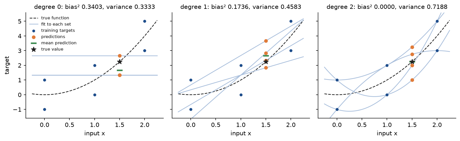
The figure shows the whole example at a glance. The distance from the green bar to the star is the bias, and the spread of the orange dots is the variance; the constant has the larger bias, the parabola the larger variance.

Three fits of the first set

For set 1, with targets (1, 2, 5):

• Degree 0 fits the mean, (1 + 2 + 5) / 3 = 2.6667, and predicts 2.6667 everywhere.
• Degree 1 fits a line. With inputs 0, 1 and 2 the least-squares slope is (y3 - y1) / 2 = (5 - 1) / 2 = 2 and the intercept is the mean target minus the slope times the mean input, 2.6667 - 2 = 0.6667, so the prediction at 1.5 is 0.6667 + 2 × 1.5 = 3.6667.
• Degree 2 has three coefficients for three points and passes through all of them: the fit is 1 + x², which predicts 3.25.

Prediction weights

Each prediction at x0 = 1.5 is a weighted sum of the three targets, and the weights do not depend on the targets. For degree 0 they are (1/3, 1/3, 1/3). For degree 1 the prediction is the mean target plus 0.5 times the slope:

so the weights are (0.0833, 0.3333, 0.5833). For degree 2 they are the Lagrange interpolation weights at 1.5:

Each set of weights sums to one. Applying them to the four target vectors gives every prediction:

• Degree 0, weights (0.3333, 0.3333, 0.3333): predictions 2.6667, 1.3333, 1.3333 and 1.3333.
• Degree 1, weights (0.0833, 0.3333, 0.5833): predictions 3.6667, 2.3333, 1.8333 and 2.8333.
• Degree 2, weights (-0.1250, 0.7500, 0.3750): predictions 3.2500, 2.7500, 1.0000 and 2.0000.

Bias, variance and the decomposition

For each degree the mean prediction over the four sets is compared with f(x0) = 2.25, and the spread of the predictions around their mean is the variance, the average of the squared deviations dividing by four:

• Degree 0: mean prediction 1.6667, bias -0.5833, bias squared 0.3403, variance 0.3333. The squared errors of the four predictions are 0.1736, 0.8403, 0.8403 and 0.8403, with mean 0.6736.
• Degree 1: mean prediction 2.6667, bias 0.4167, bias squared 0.1736, variance 0.4583. The squared errors are 2.0069, 0.0069, 0.1736 and 0.3403, with mean 0.6319.
• Degree 2: mean prediction 2.2500, bias 0, bias squared 0, variance 0.71875 exactly (23/32). The squared errors are 1.0000, 0.2500, 1.5625 and 0.0625, with mean 0.71875.

For degree 0 the deviations of the four predictions from their mean are 1, -1/3, -1/3 and -1/3, whose squares average to (1 + 3 × 1/9) / 4 = 1/3. In every row bias squared plus variance equals the mean squared error: 0.3403 + 0.3333 = 0.6736 and 0.1736 + 0.4583 = 0.6319, and for degree 2 both are exactly 23/32. That value sits exactly halfway between two four-decimal numbers, so it is given in full; the package prints it as 0.7188.

The three degrees trace the whole trade-off. The constant is far from the truth but barely moves between sets. The parabola is right on average, since f is itself a parabola, but follows every unit of noise. The line is in between and has the smallest error of the three.

Because each prediction is linear in the targets, the closed forms of the linear smoother apply: the average prediction is the weights times the true values, and the variance is σ² times the squared length of the weights, with σ² = 1. For degree 1 the average prediction is (0 + 4 + 28) / 12 = 2.6667 and the squared length of the weights is (1 + 16 + 49) / 144 = 0.4583; for degree 2 the squared length is 0.015625 + 0.5625 + 0.140625 = 0.71875. These are the values above to every digit, because the four balanced noise rows have exactly the mean and covariance that the closed forms depend on. Four training sets chosen this way give the same answer as infinitely many random ones.

A new observation at x0 adds its own noise, σ² = 1, so the expected squared error of predicting y0 is 1.6736, 1.6319 and 1.71875 for degrees 0, 1 and 2.

What the training error says

The same fits scored on their own training points:

• Degree 0: training errors 2.8889, 2.8889, 1.5556 and 6.8889, mean 3.5556, against an expected error at x0 of 1.6736.
• Degree 1: training errors 0.2222, 0.2222, 0.8889 and 0.8889, mean 0.5556, against 1.6319.
• Degree 2: training errors all 0, against 1.71875.

The training error ranks the degrees by flexibility and nothing else. The parabola fits every set perfectly and has the worst expected error at x0. The formulas of the optimism section give the same means. For degree 0 the true values deviate from their mean 5/3 by (-5/3, -2/3, 7/3), so B = (25 + 4 + 49) / 27 = 2.8889, and the expected training error is B + σ² (n - p) / n = 2.8889 + 2/3 = 3.5556. For degree 1 the least-squares line through the true values is 2x - 1/3, with residuals (1/3, -2/3, 1/3), so B = 0.2222 and the expected training error is 0.2222 + 1/3 = 0.5556. The expected errors on fresh targets at the same three inputs are B + σ² + σ² p / n, that is 4.2222, 1.8889 and 2, exceeding the training errors by 2 σ² p / n = 0.6667, 1.3333 and 2.

Every number in this section is asserted by tests/test_trace.py and tests/test_closed_forms.py, and printed by examples/worked_bias_variance.py.

The code

The package ml_landscape is plain NumPy, split into one module per idea. scikit-learn is imported only inside the functions of comparisons.py, so everything else works without it.

• arrays.py holds the array types and the checks for one-dimensional inputs and valid degrees.
• polynomials.py holds polynomial_features, fit_polynomial returning a PolynomialFit, mean_squared_error, and the prediction weights smoother_matrix and hat_matrix from which every closed form is built.
• closed_forms.py holds exact_bias_variance for fixed inputs and in_sample_errors for the training error, the error on fresh targets and their gap.
• noise.py holds sylvester_hadamard and balanced_noise, noise rows with exactly zero mean and covariance σ² times the identity.
• trace.py holds worked_example, the setup above, trace_bias_variance, which keeps every target, weight, prediction and training error of a small experiment, and format_bias_variance_trace, which prints them.
• datasets.py holds the wavy curve wavy_trend, sample_regression_data, the three input designs of training_inputs and expected_test_error, which integrates the true error of a fit on a fine grid.
• simulation.py holds simulate_bias_variance, returning a BiasVarianceEstimate with pointwise and averaged bias squared, variance, simulated test error and training error.
• splits.py holds k_fold, identical to scikit-learn's KFold when unshuffled, and shuffled_split.
• curves.py holds cross_validated_errors, learning_curve, validation_curve and one_standard_error_choice.
• workflow.py holds run_workflow, the whole workflow as one function, and compare_selection_rules, which repeats the choice of degree on fresh data sets.
• no_free_lunch.py holds the enumeration of inputs and targets, the four learners in LEARNERS, the off-training-set accuracy and the smooth and parity targets.
• gallery.py holds the eight small problems of the figure of the kinds of learning.
• pitfalls.py holds the experiments behind the Pitfalls section.
• comparisons.py builds the same models, folds and curves in scikit-learn.
• plotting.py, plot_gallery.py, plot_bias_variance.py and plot_curves.py draw every figure in the handbook's four colours and save it reproducibly.

The prediction weights of a polynomial fit are one line, and every closed form is built from them:

def smoother_matrix(x_train: ArrayLike, x_query: ArrayLike, degree: int) -> Array:
    train_features = polynomial_features(x_train, degree)
    return polynomial_features(x_query, degree) @ np.linalg.pinv(train_features)

The pseudo-inverse equals the inverse formula of the normal equations when the features are independent, and gives the minimum-norm solution, the one np.linalg.lstsq returns, when they are not. The simulation draws a training set and a fresh noisy target at every query point before fitting anything, so its random stream does not depend on the degrees requested, then fits every degree to the same training set and keeps all predictions:

for index in range(sets):
    inputs = training_inputs(train_size, design, rng, low, high)
    targets = function(inputs) + noise_sd * rng.normal(size=train_size)
    fresh = true_query + noise_sd * rng.normal(size=len(queries))
    for row, degree in enumerate(degrees):
        model = fit_polynomial(inputs, targets, degree)
        predicted = model.predict(queries)

The variance is the average of squared deviations over the training sets, dividing by the number of sets rather than one less, so that bias squared plus variance equals the mean squared error of the stored predictions exactly, as in the worked example. learning_curve follows scikit-learn's convention of training on the first m rows of each training fold, so it accepts the same list of folds and returns the same numbers.

The examples and the project import the package, so install the repository first as described in the main README. The examples each demonstrate one idea and run in a few seconds at most from the repository root:

• examples/kinds_of_learning.py solves the eight small problems, prints what each learner achieved and saves the figure of the kinds of learning.
• examples/worked_bias_variance.py prints every value of the worked example, then the same quantities from the closed forms and at the training inputs, and saves the figure of the worked fits.
• examples/bias_variance_simulation.py checks the simulation against the closed forms with fixed inputs, runs the realistic simulation over degrees 0 to 12 and saves its two figures.
• examples/learning_and_validation_curves.py computes the learning curves and the validation curves over 60 data sets, saves both figures and checks the agreement with scikit-learn.
• examples/no_free_lunch.py enumerates all 256 targets on the 3-bit inputs and prints the accuracy of the four learners.
• examples/common_mistakes.py demonstrates the pitfalls: trusting the training error, gaps in the inputs, raw powers of large inputs, learning curves on sorted rows and choosing on the test set.

python machine-learning/ml-landscape/examples/kinds_of_learning.py
python machine-learning/ml-landscape/examples/worked_bias_variance.py
python machine-learning/ml-landscape/examples/bias_variance_simulation.py
python machine-learning/ml-landscape/examples/learning_and_validation_curves.py
python machine-learning/ml-landscape/examples/no_free_lunch.py
python machine-learning/ml-landscape/examples/common_mistakes.py

The sample project, project/model_selection_study.py, is a complete model-selection study on a regression problem. It draws 300 noisy observations of the wavy curve, sets 100 of them aside as the test set before anything else, and works on the remaining 200 development rows: it measures a baseline, computes the five-fold cross-validated error of every degree from 0 to 15 with its standard error, applies both selection rules, checks the learning curve of the chosen degree, refits on all development rows and scores the test rows once. Because the data are synthetic, it then does what no real project can: it computes the true expected error of both candidate degrees, and repeats the selection on 200 fresh data sets to compare the two rules by the error of the model each would have shipped. Options such as --seed, --samples, --test-size, --noise, --max-degree, --folds, --rule and --repeats change the setup, and --figures sends the PNG to another folder so a custom run does not overwrite the one shown here; the default run takes about two seconds.

python machine-learning/ml-landscape/project/model_selection_study.py
python machine-learning/ml-landscape/project/model_selection_study.py --rule one-standard-error --noise 0.2

With the defaults the study reports, step by step:

1. Baseline: predicting the mean development target gives a test error of 0.7226.
2. Validation: the cross-validated error is lowest at degree 7, 0.1569 with a standard error of 0.0162. Degrees 5 to 12 are all within 0.005 of it, and the simplest degree within one standard error of the minimum is degree 4, at 0.1651.
3. Learning curve: for degree 7 the validation error falls from 0.8606 at 20 rows to 0.1569 at 160 rows, close to the noise floor, so more data would help little.
4. Test once: the degree-7 fit on all 200 development rows scores 0.1563 with a standard error of 0.0164 on the test rows.
5. Truth: the true expected error of that model is 0.1696; the degree-4 alternative of the one-standard-error rule would have had 0.1818.
6. Rules compared on 200 fresh data sets: the lowest cross-validated error ships models with a mean true error of 0.1689 (median degree 6, degrees 4 to 15), the one-standard-error rule 0.1739 (median degree 4, degrees 4 to 8), and the simpler choice has the lower true error on only 16 % of the data sets.

The test score lies below the noise floor of 0.16, which no model can beat on average, and below the model's true error. That is not a contradiction but the standard error at work: 100 test points measure the error only to about plus or minus 0.016. The rule comparison is an honest result too. Here the wave needs a degree of about 6 to be followed closely, and the one-standard-error rule, by preferring degree 4, buys a simpler model with a 3 % larger error. It is a preference for simplicity, worth having when a simpler model is easier to deploy or explain, not a free improvement.

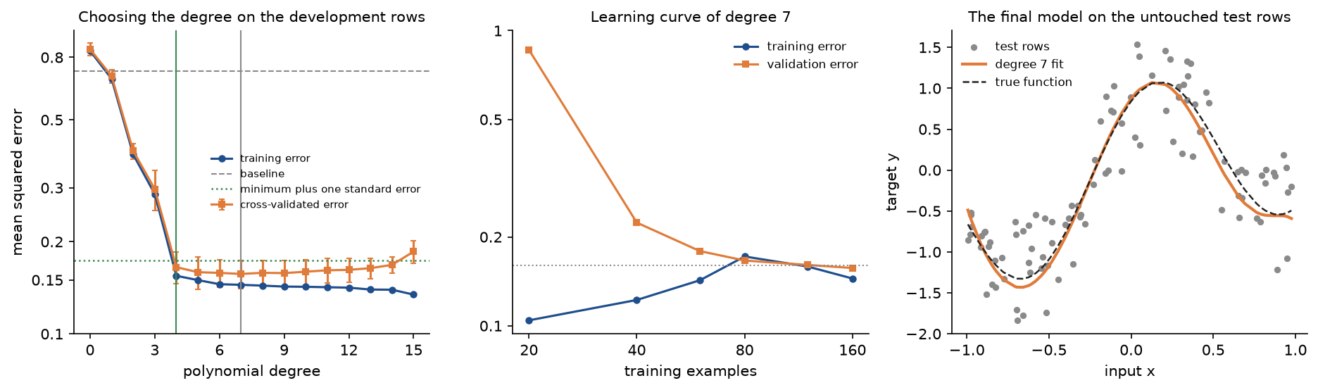
The left panel is the whole selection in one picture: the curve falls steeply to degree 4 and is then flat within its error bars, which is exactly the situation the one-standard-error rule was made for.

The notebook ml_landscape.ipynb is a guided tour in the order of this page: the kinds of learning, the worked example and its closed forms, the simulation checked against the closed forms, learning and validation curves, the workflow and the two selection rules, the no-free-lunch enumeration, each pitfall and the same helpers in scikit-learn. The tests in tests check the worked example value by value, the mathematical properties above, the numbers of the project and the agreement with scikit-learn, and run in a few seconds:

python -m pytest machine-learning/ml-landscape

Every data set on this page is synthetic, generated from a fixed seed by the package, so nothing is downloaded and no licence is involved.

In practice

PolynomialFeatures followed by LinearRegression is the library version of fit_polynomial, and learning_curve and validation_curve in sklearn.model_selection are the library versions of the two curve helpers. scikit-learn scorers follow the convention that larger is better, so the mean squared error comes back negated:

from sklearn.linear_model import LinearRegression
from sklearn.model_selection import learning_curve, validation_curve
from sklearn.pipeline import make_pipeline
from sklearn.preprocessing import PolynomialFeatures

model = make_pipeline(PolynomialFeatures(4, include_bias=False), LinearRegression())
sizes, train_scores, valid_scores = learning_curve(
    model,
    x[:, None],
    y,
    train_sizes=[15, 50, 200, 800],
    cv=folds,
    scoring="neg_mean_squared_error",
)
train_scores, valid_scores = validation_curve(
    make_pipeline(PolynomialFeatures(include_bias=False), LinearRegression()),
    x[:, None],
    y,
    param_name="polynomialfeatures__degree",
    param_range=range(1, 13),
    cv=folds,
    scoring="neg_mean_squared_error",
)

Given the same folds on the 1000 points of the learning curves, examples/learning_and_validation_curves.py finds that the predictions agree with fit_polynomial to 5.2 × 10⁻¹⁴ over degrees 1 to 10, the learning curve of degree 4 to 2.2 × 10⁻¹⁵ and the validation curve over degrees 1 to 12 to 2.6 × 10⁻¹⁵, and that unshuffled k_fold produces exactly the folds of KFold. tests/test_comparisons.py asserts the same on other data. LearningCurveDisplay and ValidationCurveDisplay draw the same curves directly from an estimator. scikit-learn has no function that estimates bias and variance by resampling; the simulation here needs the true function, which only synthetic data provides.

Every model in this handbook has a setting that plays the role of the polynomial degree, and the bias-variance reasoning above applies to each of them. Each item names the setting and the direction that buys lower bias at the price of higher variance:

• Linear and polynomial regression: a higher degree or a weaker ridge penalty (Linear regression).
• k-nearest neighbours: fewer neighbours (k-nearest neighbours).
• Decision trees: deeper trees and smaller leaves (Decision trees).
• Bagging and random forests: averaging more trees lowers the variance and leaves the bias unchanged (Ensembles).
• Boosting: more rounds or a larger learning rate (Ensembles).
• Support vector machines: a larger penalty C or a narrower kernel (Support vector machines).
• Neural networks: wider and deeper networks, longer training, less weight decay and dropout (Regularization).
• Clustering and PCA: more clusters or more components kept (Clustering, Dimensionality reduction).

When to use which:

• Use the from-scratch helpers to see where bias and variance come from, to check a closed form against a simulation, and to experiment with designs and noise levels on problems whose truth is known.
• Use scikit-learn's learning_curve and validation_curve, inside a Pipeline so that preprocessing is refitted on every fold, for real data. Pass shuffle=True to learning_curve, or shuffle the rows yourself, unless the rows are in random order.
• Prefer cross-validation over a single train and validation split for choosing capacity, and report the standard error with every cross-validated score. Prefer the one-standard-error rule when the curve is flat near its minimum and a simpler model is easier to deploy or explain, knowing that it may cost a little accuracy, as the project measured.
• The U-shaped validation curve describes models with fewer parameters than training examples, the regime of this page. Far beyond the point where a model can interpolate its training data, test error can fall again as parameters are added, the double descent observed in large neural networks; the reference by Belkin and colleagues below treats it.

Pitfalls

• Judging a model by its training error. Training error falls with every added parameter and says nothing once the model can interpolate. In the simulation, degree 12 has a training error of 0.0549, a third of the noise floor, and an expected error of 4.5691, twenty-one times that of degree 4. In the worked example the interpolating parabola has zero training error and the largest expected error. examples/common_mistakes.py prints both.
• Choosing on the test set and reporting the same number. Over 300 repetitions with 30 training and 30 test points, choosing the degree with the lowest test error reports an average of 0.1913, while the chosen models' true expected error averages 0.2255; the reported score is too low in 66 % of repetitions (examples/common_mistakes.py). Data leakage and pitfalls quantifies this optimism in general.
• Reading too much into a test score. In the project the test score, 0.1563, is below the noise floor of 0.16 that no model can beat on average, because 100 test points measure the error only to about plus or minus 0.016. Report the standard error with every test score, and do not treat differences smaller than it as findings.
• Expecting more data to fix bias. The degree-1 learning curve is flat at about 0.66 from 50 to 800 examples. When training and validation error have met far above the noise level, the fix is capacity or better inputs, not data. Conversely, when the gap is large, as for degree 10, more data is often the cheapest fix.
• Trusting a validation curve from one data set. Over 30 data sets of 40 points, the degree chosen by cross-validation ranged from 4 to 11 (examples/learning_and_validation_curves.py). Look at the standard errors of the cross-validated scores, and when the curve is flat near its minimum, the simpler model is usually the safer choice.
• Extrapolating with a flexible model. Drawing the 20 training inputs uniformly at random instead of one per bin sometimes leaves a gap near an end of the interval, and polynomials extrapolate wildly into gaps. At degree 4 the variance rises fivefold, from 0.0433 to 0.2162; at degree 8 the average variance rises from 0.1531 to about 1320, while the median test error only rises from 0.2594 to 0.6925, because a few training sets produce enormous errors (examples/common_mistakes.py). Check where the model will be asked to predict against where it has data.
• Polynomial features of unscaled inputs. For 40 inputs between 0 and 50, the feature matrix of degree 12 has a condition number around 10²², far beyond the roughly 10¹⁶ that double precision can resolve, so even that number is only an order of magnitude. The solver discards directions it cannot resolve, and the degree-12 fit has a training error of 0.1640, fifty times that of the degree-8 fit, which is impossible for nested least squares. Rescaled to the interval from -1 to 1, the condition number is 1.7 × 10⁴ and the training error 0.0031. Scale inputs before building powers, or use an orthogonal polynomial basis.
• Learning curves on sorted rows. learning_curve, ours and scikit-learn's, trains on the first rows of each training fold. On rows sorted by the input, the degree-4 validation error at 20 training rows is 1.8 × 10⁷, against 0.2187 in random order, because the small training sets see only one end of the interval (examples/common_mistakes.py).
• Applying the additive decomposition to other losses. Bias squared plus variance plus noise is an identity for squared error only. Under the zero-one loss of classification, variance can lower the error when the bias is large: at an input whose label is 1, a classifier that always predicts 0 is wrong every time, while one that predicts 0 on 60 % of training sets and 1 on the rest is wrong only 60 % of the time. Decompositions for other losses exist but are not additive in the same way (Domingos, 2000).
• Reading no free lunch as "all methods are equal". The theorem averages over all targets, almost all of which are patternless. On the smooth targets of the enumeration, nearest neighbour is right 81 % of the time and majority vote 44 %; on parity the ranking reverses. The theorem is an argument for validating on data from the problem at hand, not against choosing methods.

Further reading

• T. M. Mitchell, Machine Learning, McGraw-Hill, 1997, chapter 1. The experience, task and performance definition of learning.
• T. Hastie, R. Tibshirani and J. Friedman, The Elements of Statistical Learning, second edition, Springer, 2009, chapters 2 and 7. The bias-variance decomposition, the optimism of the training error, Cp, cross-validation and the one-standard-error rule.
• C. M. Bishop, Pattern Recognition and Machine Learning, Springer, 2006, sections 1.1, 1.3 and 3.2. Polynomial curve fitting, model selection and the bias-variance decomposition.
• S. Geman, E. Bienenstock and R. Doursat, "Neural networks and the bias/variance dilemma", Neural Computation 4(1), 1-58, 1992. The paper that made the decomposition central to machine learning.
• D. H. Wolpert, "The lack of a priori distinctions between learning algorithms", Neural Computation 8(7), 1341-1390, 1996. The no-free-lunch theorems for supervised learning.
• S. Shalev-Shwartz and S. Ben-David, Understanding Machine Learning: From Theory to Algorithms, Cambridge University Press, 2014, chapters 2 to 5. Empirical risk minimization, the approximation-estimation decomposition and a formal no-free-lunch theorem.
• P. Domingos, "A unified bias-variance decomposition and its applications", ICML 2000. Bias and variance for zero-one and other losses.
• P. Domingos, "A few useful things to know about machine learning", Communications of the ACM 55(10), 78-87, 2012. Practical consequences of generalization, overfitting and inductive bias.
• M. Belkin, D. Hsu, S. Ma and S. Mandal, "Reconciling modern machine-learning practice and the classical bias-variance trade-off", Proceedings of the National Academy of Sciences 116(32), 15849-15854, 2019. Double descent beyond the interpolation threshold.
• C. L. Mallows, "Some comments on Cp", Technometrics 15(4), 661-675, 1973.
• R. S. Sutton and A. G. Barto, Reinforcement Learning: An Introduction, second edition, MIT Press, 2018, chapters 1 and 2. Learning from rewards, starting with the multi-armed bandit shown in the figure of the kinds of learning.