Data leakage and pitfalls¶

A model is only as good as the evaluation that vouches for it, and the commonest way to get a wonderful number for a useless model is leakage: information that will not exist when the model is used reaches it during training, preprocessing or model selection. Leaks rarely announce themselves. A scaler fitted before the split, a column recorded after the outcome, two recordings of the same person on both sides of the split or a test set consulted once too often all produce scores that look like progress. This page explains what leakage is and derives why it biases scores upwards, works a ten-row example by hand in which feature selection on all rows turns a coin flip into a perfect score, and then demonstrates fifteen pitfalls one at a time, each with a wrong pipeline, a right pipeline and both scores, on synthetic data you can regenerate. A sample project audits a realistic study export for leaks, repairs it and shows what the honest number was all along. Afterwards you will be able to recognise each kind of leak, measure how much it inflates a result, detect it with a few cheap checks and build evaluations that cannot leak by construction. It builds on Evaluation metrics, and its models come from k-nearest neighbours, Logistic regression and Naive Bayes.

To run the code in this topic, install the base group, and the ml group for the comparisons with scikit-learn.

Intuition¶

An evaluation is a rehearsal of deployment. On the day the model is used it will see a new input, it will know only what was knowable before the prediction, and nobody will have tuned anything on the answer. A test score means something only if the evaluation reproduces those three conditions. Leakage is any way in which it does not: the model, its preprocessing or a decision about it has seen information from the evaluation data, from the future or from the label itself. The result is a forecaster scored on days whose weather it has already seen.

Leaks inflate scores rather than merely adding noise, because learning is optimization. A model takes whatever lowers its training loss, and a shortcut that also exists in the test rows lowers the test loss too. A token that the labelling process left in the text, a patient identifier, a row number that follows the label, the training-set twin of a test row: all of them are easier to learn than the real relationship, so a flexible model finds them first. The same happens one level up when people try many models and keep the one that scores best on the test set, because the selection itself fits the noise in those test rows.

Leaks reach an evaluation through four channels, and the rest of the page is organized by them:

The evaluation rows shape the model. Test or validation rows take part in fitting, preprocessing, augmentation or the choice of model. Examples: preprocessing fitted before the split, the test set used for selection, augmentation before the split.
Features that will not exist at prediction time. A column is recorded after the outcome, or is a by-product of how the labels were made. Examples: target leakage, proxy tokens, identifiers and ordering artefacts.
Test rows that are not new. Test rows are copies or relatives of training rows. Examples: duplicates and near duplicates, the same subject on both sides, neighbouring points of a time series.
A score that answers the wrong question. The procedure is sound but the number misleads. Examples: accuracy under class imbalance, random transforms of the evaluation data, a shift between training and deployment data.

The diagram is an honest evaluation with the four leak routes drawn in orange. Each route breaks one link of the rehearsal: route 2 adds information that use will not have, routes 1 and 3 stop the test rows from being unseen, and route 4 measures something other than what use will need.

The cure is the same in every case. Decide how future data will arrive, split the data so that the test rows arrive in the same way, put every step that learns from data inside the training side of every split, and look at the evaluation data only once at the end.

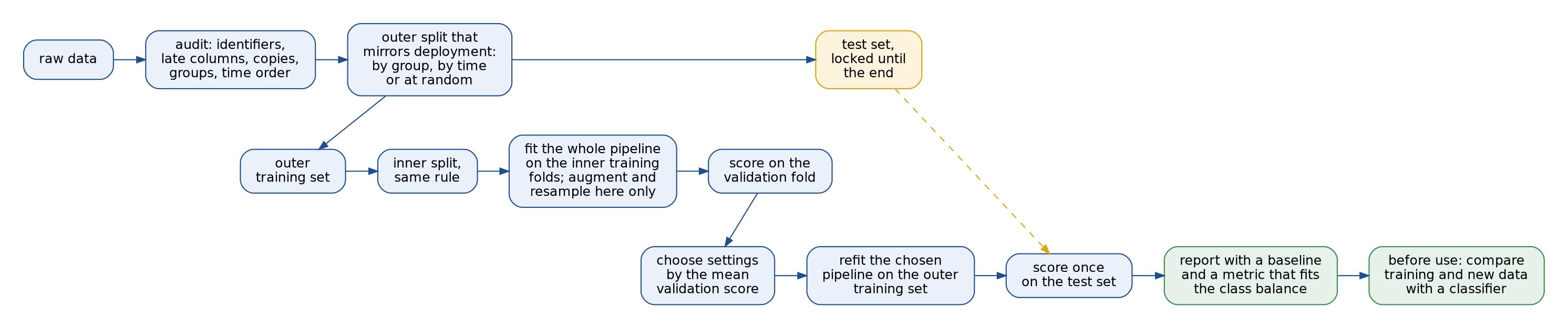
The workflow is the template for the rest of the page. The locked test set touches the procedure exactly once, at the end; everything that learns or chooses happens inside the outer training set, and the inner split follows the same rule as the outer one.

How it works¶

Notation¶

Two-class problems are used throughout. The quantities are:

D, the distribution of input and label pairs (x, y) the model will meet in use.
S and T, the training set and the test set, with m rows in the test set.
A, the learning procedure: everything between raw data and fitted model, including preprocessing, feature selection and every choice of setting. The fitted model is f = A(S).
The loss ℓ of one prediction. The 0-1 loss, one for a wrong prediction and zero for a right one, gives accuracy as one minus its mean.
π, the share of positive examples, and TPR and TNR, the true positive rate (recall of the positive class) and the true negative rate.

The risk R(f) is the expected loss in use, and the test estimate averages the loss over the test rows:

The risk R of f is the expected loss of f of x against y over pairs drawn from D; the test estimate R hat of f is one over m times the sum over the test rows of the loss of each prediction

Every argument on this page is about whether the second number is a fair estimate of the first.

A clean test set gives an unbiased estimate¶

Suppose the rows of T are drawn independently from D and f was computed without them. Conditional on f, each term of the test estimate is then an independent draw of a random variable whose mean is the risk, so

The expected test estimate given f is one over m times the sum over the test rows of the expected loss given f, which is the risk R of f

For the 0-1 loss with true accuracy a, the number of correct test predictions is binomial and the measured accuracy has a known spread:

The number of correct predictions follows a binomial distribution with m trials and success probability a, and the standard deviation of the measured accuracy is the square root of a times 1 minus a over m

The derivation needs two things: f must not depend on T, and T must be drawn the way deployment data will be drawn. Leakage breaks one or the other. Once the procedure that produced f has looked at the test rows, the terms are no longer draws with mean R(f); once the test rows are relatives of the training rows, they are draws from a different, easier distribution.

Choosing among candidates on the same data¶

Let f1 to fK be candidate models, for example one per setting of a hyperparameter, all scored on the same test set, and suppose the best score is reported. For every j the smallest estimate is at most the estimate of candidate j; taking expectations and then the minimum over j gives

The expected smallest test estimate among the K candidates is at most the smallest expected test estimate, which is the smallest true risk

The reported error is optimistic for the best candidate, and equality needs every estimate to be free of noise. In accuracy terms, the expected best score exceeds the best true accuracy. The size of the effect follows from the distribution of a maximum. Take K independent candidates with the same true accuracy p, let Ck be the number of test rows candidate k gets right, which is binomial, and let M be the largest of them. Any count with values from 0 to m equals the number of thresholds c from 1 to m that it reaches, and M stays below c exactly when every candidate does, which has probability F(c - 1) to the power K by independence, with F the binomial distribution function:

M, the largest count, equals the sum over c from 1 to m of the indicator that M is at least c; so the expected value of M is the sum of the probabilities that M is at least c, which is the sum over c of 1 minus F of c minus 1 to the power K

Dividing by m gives the expected best accuracy, which expected_best_accuracy computes exactly. A normal approximation shows how it scales:

The expected best accuracy is approximately p plus the square root of p times 1 minus p over m, times e K; e K is the integral over x of x times K times the standard normal density at x times the standard normal distribution function at x to the power K minus 1

The integrand contains the density of the largest of K standard normal variables, so e_K is the mean of that maximum; it grows roughly like the square root of 2 ln K. The optimism shrinks with the square root of the test-set size and grows without bound, though slowly, with the number of candidates. Real candidates share training and test rows and are positively correlated, which makes the effect smaller than in this independent case but never removes it.

Selecting features on all rows¶

The same maximum hides inside feature selection. For n rows and a feature unrelated to the label, the sample correlation r between feature and label is approximately normal, and the largest of p such correlations follows from the same extreme-value argument:

Each correlation r j is approximately normal with mean 0 and variance 1 over n, and the largest absolute correlation among p features is approximately the square root of 2 ln p over n

For n = 100 and p = 10,000 that is 0.4292, a correlation that would count as a useful predictor in most applications. If the selection runs on all n rows before cross-validation, the labels of the rows that later serve as test folds helped choose the features, so the chosen features agree with those labels by construction. Cross-validation after the selection then measures how well the features fit labels they were chosen to fit. When the selection runs inside each training fold instead, the held-out labels play no part and the score returns to chance.

Dependent rows and the unit of sampling¶

Deployment defines the unit that arrives new: a new patient, a new day, a new document. If each subject contributes r rows and rows are split at random into k folds, a test row's subject is absent from the training folds only if its other r - 1 rows all land in the same test fold:

The probability that a test row has no relative in training is approximately one over k to the power r minus 1

For r = 10 and k = 5 that is 5.1 × 10⁻⁷: essentially every test row has relatives in training. A random split then estimates the risk on subjects the model has already met, not on new ones. The same holds for a time series, where the test point at time t has its neighbours at t - 1 and t + 1 in training whenever the split ignores time, and the estimate measures interpolation instead of forecasting. The split must draw its test rows the way deployment draws them: by subject, by time, by site.

Accuracy, prevalence and the baseline¶

Accuracy mixes the two error rates in proportion to the class shares:

Accuracy is pi times the true positive rate plus 1 minus pi times the true negative rate; balanced accuracy is one half of the sum of the true positive rate and the true negative rate

A classifier that always predicts the negative class has TPR = 0 and TNR = 1, so its accuracy is 1 - π: 0.97 when positives make up 3 % of the data. Balanced accuracy is 0.5 for every constant classifier, whatever π is, and recall, precision and the area under the ROC or precision-recall curve all expose a classifier that ignores the minority class. Under imbalance, accuracy mostly measures the true negative rate. Evaluation metrics treats these measures in depth.

Detecting a shift with a classifier¶

Label every training row 0 and every row of the new data 1, and train a classifier to tell them apart. If the two sets come from the same distribution, the probability that a row is new does not depend on its inputs, so no classifier can do better than chance on held-out rows:

If the probability of being new given x equals n1 over n0 plus n1 for every x, the expected area under the ROC curve is one half

An area well above 0.5 on held-out folds proves the inputs differ, and the classifier's weights show where. This is adversarial validation. The area under the curve is the probability that a randomly chosen positive scores higher than a randomly chosen negative, ties counting one half, and it equals the Mann-Whitney statistic, which roc_auc computes from ranks:

U is the sum of the ranks of the positive scores minus n1 times n1 plus 1 over 2, and the AUC is U divided by n1 times n0

The scores of all n1 + n0 rows are ranked together from 1, tied scores share the mean of their ranks, and n1 and n0 count positives and negatives. Two caveats matter in practice. The check compares the input distributions only: if the relation between input and label changes while the inputs keep their distribution, the area stays at 0.5 and the model can still fail. And the held-out folds of the adversarial classifier must respect the groups in the data, otherwise it wins by recognising subjects it has already seen, which the Pitfalls section measures.

Worked example¶

Ten rows, four features drawn uniformly from the integers 1 to 9 independently of the labels, so no feature carries any information about the class. Rows 1 to 6 are for training and rows 7 to 10 for testing. Each row below gives the four features x1 to x4 and the label:

Training rows: row 1 (3, 1, 8, 4) label 0; row 2 (7, 2, 3, 2) label 1; row 3 (9, 5, 8, 9) label 1; row 4 (3, 1, 1, 8) label 0; row 5 (8, 3, 6, 1) label 1; row 6 (5, 2, 3, 3) label 0.
Test rows: row 7 (8, 9, 8, 6) label 1; row 8 (9, 9, 4, 6) label 0; row 9 (5, 8, 1, 8) label 0; row 10 (1, 6, 9, 6) label 1.

The procedure is the smallest possible version of "select a feature, then classify". It keeps the single feature j with the largest gap between the two class means, and classifies each test row by the nearer of the two training class means of that feature, a nearest-centroid classifier in one dimension whose threshold is the midpoint of the two means:

The gap of feature j is the absolute difference between its class-1 mean and its class-0 mean; the threshold t is half the sum of the two class means, and a row is predicted 1 when it is nearer the class-1 mean

The two orders side by side: the leaky run chooses the feature on all ten rows, which picks x3, then splits and scores 1.0000; the honest run splits first, chooses on the six training rows, which picks x1, and scores 0.5000

The two runs differ in one step only, which rows choose the feature. In both, the class means used for classifying come from the six training rows.

The leaky way: select on all ten rows¶

Class 1 is rows 2, 3, 5, 7 and 10; class 0 is rows 1, 4, 6, 8 and 9. Each class has five rows, so the means are easy:

x1: class 1 sums 7 + 9 + 8 + 8 + 1 = 33, mean 6.6; class 0 sums 3 + 3 + 5 + 9 + 5 = 25, mean 5.0; gap 1.6.
x2: class 1 sums 25, mean 5.0; class 0 sums 21, mean 4.2; gap 0.8.
x3: class 1 sums 3 + 8 + 6 + 8 + 9 = 34, mean 6.8; class 0 sums 8 + 1 + 3 + 4 + 1 = 17, mean 3.4; gap 3.4.
x4: class 1 sums 24, mean 4.8; class 0 sums 29, mean 5.8; gap 1.0.

Feature x3 wins clearly. The classifier is then trained, correctly, on the training rows only: the class-0 mean of x3 over rows 1, 4 and 6 is (8 + 1 + 3) / 3 = 4.0000 and the class-1 mean over rows 2, 3 and 5 is (3 + 8 + 6) / 3 = 5.6667, so the threshold is their midpoint, 4.8333. The test values of x3 are 8, 4, 1 and 9, giving predictions 1, 0, 0 and 1, and the true labels are 1, 0, 0 and 1. Test accuracy 1.0000.

The honest way: select on the six training rows¶

Now class 1 is rows 2, 3 and 5 and class 0 is rows 1, 4 and 6:

x1: class 1 mean (7 + 9 + 8) / 3 = 8.0000, class 0 mean (3 + 3 + 5) / 3 = 3.6667, gap 4.3333.
x2: class 1 mean 3.3333, class 0 mean 1.3333, gap 2.0000.
x3: class 1 mean 5.6667, class 0 mean 4.0000, gap 1.6667.
x4: class 1 mean 4.0000, class 0 mean 5.0000, gap 1.0000.

The training rows prefer x1, with class means 3.6667 and 8.0000 and threshold 5.8333. The test values of x1 are 8, 9, 5 and 1, giving predictions 1, 1, 0 and 0 against true labels 1, 0, 0 and 1. Test accuracy 0.5000, exactly the coin flip that noise deserves.

What happened¶

The training rows rank x3 third. It reached first place only because the four test rows were counted: on their own, their x3 values put the class-1 mean at (8 + 9) / 2 = 8.5 and the class-0 mean at (4 + 1) / 2 = 2.5, a gap of 6.0. The leaky procedure chose the feature on which the test labels happened to line up, and then congratulated itself for predicting them. Nothing in the classifier was fitted on the test rows; one choice made before the split was enough. With four features and four test rows the effect is a lucky draw; with thousands of features it is a certainty, as the section on feature selection below shows.

How large the optimism of choosing on the test set is¶

Thirty candidate models, each with true accuracy p = 0.5, are scored on the same m = 80 test rows, and the best score is reported. The numbers:

The standard deviation of one candidate's score is the square root of 0.5 × 0.5 / 80, which is 0.0559.
The expected largest of 30 standard normal variables is e_30 = 2.0428. For comparison, the square root of 2 ln 30 is 2.6081, an overestimate at this small K.
The normal approximation gives 0.5 + 0.0559 × 2.0428 = 0.6142, and the exact binomial sum gives 0.6137.
One candidate reaches at least 0.6, that is 48 or more of the 80 rows, with probability 0.0465. At least one of the thirty does with probability 1 - (1 - 0.0465) to the power 30, which is 0.7603 from the rounded term and 0.7600 at full precision.

So the test-set winner of thirty useless models "beats chance by ten points" three times out of four. In a simulation, thirty nearest-neighbour candidates on 100 pure-noise data sets average a best score of 0.6085 (standard deviation 0.0286), slightly below the formula because those candidates share their data and are correlated.

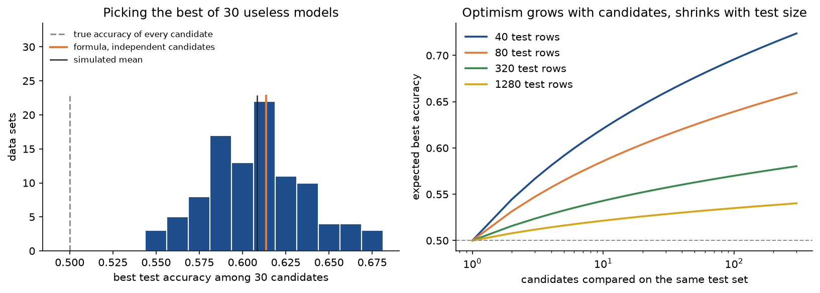
The left panel is the simulation; the right panel is the exact formula for other sizes. The optimism grows with the number of candidates and shrinks with the size of the test set, but even 1280 test rows leave a few points of optimism after a few hundred candidates. Every number in this section is asserted by tests/test_worked_example.py, tests/test_selection_bias.py and tests/test_fitting_leaks.py, and printed by examples/worked_example.py.

The code¶

The package data_leakage_and_pitfalls is a small evaluation library written from scratch in NumPy, so that each leak can be shown as a one-line difference between two pipelines. scikit-learn is imported only inside the two comparison modules. The modules, from the bottom up:

arrays.py holds the array types and as_matrix, which insists on one example per row.
metrics.py holds accuracy, recall, precision, balanced accuracy, the ROC AUC through average_ranks in its Mann-Whitney form, and the mean absolute error.
splits.py holds shuffled_split, k_fold, group_k_fold and time_series_split; the last three reproduce scikit-learn's KFold, GroupKFold and TimeSeriesSplit index for index.
preprocessing.py holds the steps that never read labels: Standardizer, PrincipalComponents, KeepColumns, DropColumns and BagOfWords.
supervised_steps.py holds the steps that do: the ANOVA F score with SelectBestFeatures (as SelectKBest(f_classif)), the mean gaps of the worked example, and TargetMeanEncoder.
neighbours.py and linear_models.py hold the models: NearestCentroid, KNeighboursClassifier, KNeighboursRegressor, LogisticRegression (Newton's method with an L2 penalty and optional class balancing) and MultinomialNaiveBayes.
pipeline.py holds Pipeline, and evaluation.py the procedures that score it: holdout_score, cross_validate, out_of_fold_outputs, select_on_test (the wrong way to tune) and nested_cross_validate (the right way, with optional groups for the inner loop).
diagnostics.py holds the cheap checks: adversarial_validation (with optional groups), single_feature_auc, near_duplicate_groups (union-find over pairs closer than a tolerance), cross_contamination and group_overlap.
selection_bias.py holds the arithmetic of choosing: the exact expected_best_accuracy, chance_best_reaches, expected_maximum_of_normals, normal_best_accuracy and the chance correlations of many features.
worked_example.py holds the ten rows, trace_selection and format_selection_trace.
datasets.py generates data without a leak of their own, and leaky_datasets.py one data set per leak: kiosk reviews, loan applications, jittered and duplicated rows, a sorted export and three acquisition sites.
fitting_leaks.py, feature_leaks.py, row_leaks.py and score_traps.py hold one experiment per pitfall, grouped by the four channels, each returning a LeakResult from results.py with the leaky score, the honest score and the extra measurements. catalogue.py runs them all.
realistic_run.py holds the combined analysis of the sample project, and study_export.py the messy export the project audits.
audit_plan.py, audit_checks.py and audit.py are the leakage audit: the data set and the written-down evaluation plan, six checks, and the report.
comparisons.py and comparisons_evaluation.py run the same pieces in scikit-learn.
plotting.py and plotting_leaks.py draw every figure in the handbook's four colours.

Every step and model is a frozen dataclass whose fit returns a new, fitted copy, so an unfitted pipeline can be reused for every fold without state leaking from one fold into the next. A Pipeline fits each step on the output of the previous one, using only the rows it is given:

def fit(self, features: Any, labels: Array) -> Pipeline:
    fitted = []
    current = features
    for step in self.steps[:-1]:
        step = step.fit(current, labels)
        current = step.transform(current)
        fitted.append(step)
    fitted.append(self.steps[-1].fit(current, labels))
    return Pipeline(tuple(fitted))

cross_validate calls fit on the training indices of each split and scores the test indices, so the difference between a leaky and an honest evaluation is visible in the code. On 100 rows of 10,000 pure-noise features:

import data_leakage_and_pitfalls as lp

features, labels = lp.noise_dataset(100, 10_000, seed=0)
folds = lp.k_fold(100, 5, seed=0)

selected = lp.SelectBestFeatures(20).fit(features, labels).transform(features)
leaky = lp.cross_validate(lp.NearestCentroid(), selected, labels, folds)

pipeline = lp.Pipeline((lp.SelectBestFeatures(20), lp.NearestCentroid()))
honest = lp.cross_validate(pipeline, features, labels, folds)

leaky.mean() is 0.9300 and honest.mean() is 0.5800 for this draw.

The examples and the project import the package, so install the repository first as described in the main README. The examples each demonstrate one idea and run in a few seconds from the repository root:

examples/worked_example.py prints every value of the worked example, the arithmetic of choosing the best of 30 candidates and the simulation, and saves the selection-bias figure.
examples/fitting_leaks.py runs the leaks through fitting: feature selection for a growing number of noise features, PCA and scaling, the reused test set, augmentation, random test-time transforms and target encoding, and saves two figures.
examples/feature_and_row_leaks.py runs the proxy token, target leakage and identifier experiments with their single-feature screens, then the time series, the subjects and the near duplicates, and saves the time-series figure.
examples/score_traps.py runs the accuracy paradox and the site shift, saves the adversarial-validation figure, and shows adversarial validation with and without grouped folds.
examples/leak_catalogue.py runs every experiment, prints one line per leak and saves the summary figure.
examples/compare_with_sklearn.py checks every piece against scikit-learn.

python machine-learning/data-leakage-and-pitfalls/examples/worked_example.py
python machine-learning/data-leakage-and-pitfalls/examples/fitting_leaks.py
python machine-learning/data-leakage-and-pitfalls/examples/feature_and_row_leaks.py
python machine-learning/data-leakage-and-pitfalls/examples/score_traps.py
python machine-learning/data-leakage-and-pitfalls/examples/leak_catalogue.py
python machine-learning/data-leakage-and-pitfalls/examples/compare_with_sklearn.py

The sample project: a leakage audit¶

project/leakage_audit.py is a small audit tool. It takes a data set, a written description of how the data will be evaluated and, optionally, a sample of the data the model will meet in use, runs six checks and prints a report in which each finding is a leak, a warning, ok, or skipped when the inputs do not allow the check.

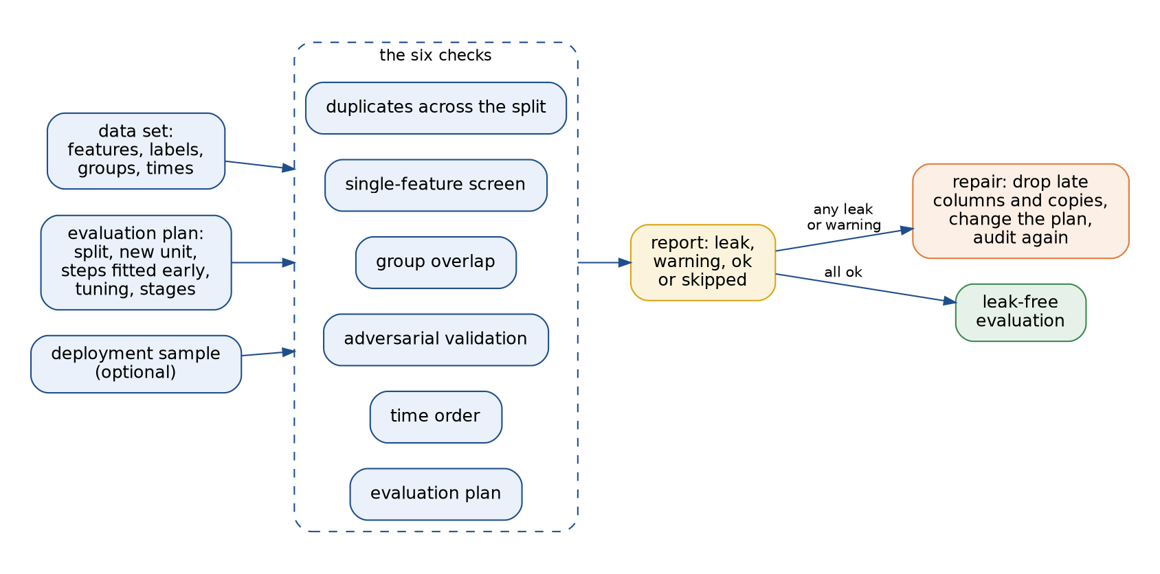
The audit takes a data set with features, labels, groups and times, an evaluation plan with the split, the unit that is new in use, the steps fitted early, the tuning and the stages, and an optional deployment sample; six checks produce a report of leaks, warnings, ok and skipped findings, which leads either to a repair and a second audit or to a leak-free evaluation

The evaluation plan is a small record, EvaluationPlan, that writes down what is usually left implicit: how test rows are drawn (random, grouped or time), what will be new in use (a row, a whole group or a later period), which steps are fitted on all rows before the split, whether the reported score also chose the settings, how an inner tuning loop splits, and when each column becomes known compared with the moment of prediction. The six checks are:

Duplicates across the split: rows that repeat an earlier row, and the share of test rows, averaged over the folds, that have a copy in training. Copies across the split are a leak; copies that the split keeps together are a warning.
Single-feature screen: the ROC AUC of every column used alone against the label. A column is named when it reaches 0.95, or when it is the best column and leads every other one by at least 0.15.
Adversarial validation against the deployment sample, twice: one classifier on every column, with folds grouped when groups are given, and every column on its own with the same naming rule. With many columns and few subjects the classifier is noisy, while a column that is filled in during development and empty in use stands out at once on its own.
Group overlap: the share of test rows whose group is also in training, a leak when every group will be new in use.
Time order: columns that become known after the moment of prediction, and, when the model will predict the future, test rows that come before training rows.
The evaluation plan itself: steps fitted before the split, a reported score that also chose the settings, and an inner loop that splits differently from the outer one.

By default the project audits the export of a realistic study: 36 subjects with 10 recordings each and 200 measurements, of which 10 carry a signal, as realistic_cohort generates them. The export adds what real exports add. A column follow_up_visits counts the visits booked after the diagnosis, at least one for every positive subject. Thirty recordings appear twice. A sample of recordings from 40 new subjects comes with it, whose follow-up column is still empty, written as -1, because nothing has been booked when a prediction is made. The plan is the naive analysis: select 20 features on all rows, split recordings at random into five folds, and choose the number of neighbours of a nearest-neighbour model by the same cross-validated score that is reported. The first audit finds:

Duplicates across the split, a leak: 30 rows repeat an earlier row, and 11.3 % of test rows have an exact copy in training.
Single-feature screen, a warning: follow_up_visits alone reaches a ROC AUC of 1.0000; the best measurement, m007, reaches 0.9064.
Adversarial validation, a warning: the classifier reaches only 0.7232, although its largest weight by far is on follow_up_visits (-2.9930 against at most 0.9219 for a measurement); on its own the follow-up column separates the two samples perfectly, 1.0000.
Group overlap, a leak: 100.0 % of test rows have their subject in training, while every subject will be new in use.
Time order, a leak: follow_up_visits is known at follow-up, after the prediction at intake.
The evaluation plan, a leak: feature selection is fitted before the split, and the reported score also chose the settings.

On this export the naive analysis reports a perfect 1.0000. The repairs the report asks for are to drop the column known only at follow-up, drop the repeated recordings and evaluate with folds grouped by subject, inside and out. The repaired data are exactly the cohort, and the second audit finds nothing: the best measurement alone reaches 0.8983, the grouped adversarial classifier 0.4780 with no column standing out (the largest alone 0.6933), and no test row has a copy or its subject in training.

Then the project runs both analyses on the repaired data and checks them against what they claim. The leak-free analysis puts scaling, F-score selection of 10, 20 or 50 features and 5 or 15 neighbours in one pipeline, tunes it in a five-fold inner loop grouped by subject and scores it on six outer folds grouped by subject:

The naive analysis still reports 1.0000, for every number of neighbours from 1 to 15.
The leak-free estimate is 0.7556, from outer folds of 0.8667, 0.8167, 0.8667, 0.5833, 0.7167 and 0.6833; its inner loops report a believable 0.7383 on average.
The deployed model, the setting with the best grouped score on all 36 subjects (10 features and 15 neighbours) refitted on every recording, scores 0.8150 on 40 new subjects. The naive analysis's own model scores 0.7725 there.
Shuffling the labels between subjects is a cheap audit of a whole procedure: labels that mean nothing must give chance. The naive analysis still reports 0.9972, the leak-free one 0.4722.

python machine-learning/data-leakage-and-pitfalls/project/leakage_audit.py
python machine-learning/data-leakage-and-pitfalls/project/leakage_audit.py --write-example .data/data-leakage-and-pitfalls
cd .data/data-leakage-and-pitfalls
python ../../machine-learning/data-leakage-and-pitfalls/project/leakage_audit.py --csv study-export.csv --group subject --plan naive-plan.json --deployment deployment.csv

The default run takes about two seconds. --write-example writes the export, the deployment sample and both plans as CSV and JSON files, here into the repository's ignored .data folder, and --csv audits any table with a header row and numbers in every field, with --label, --group and --time naming the special columns and --plan and --deployment the other inputs; on the written files it reproduces the report above. --copies and --seed change the export, and --figures sends the two PNGs to another folder so a custom run does not overwrite the ones shown here.

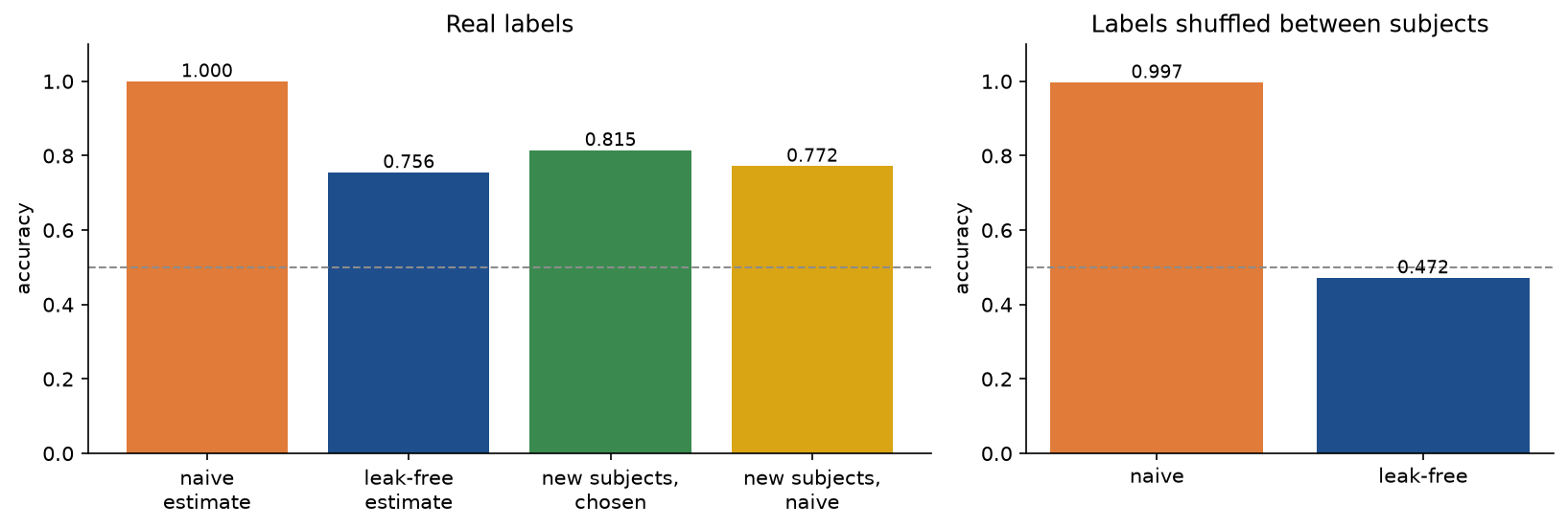
Left: bars of accuracy for the naive estimate at 1.000, the leak-free estimate at 0.756, the chosen model on new subjects at 0.815 and the naive model on new subjects at 0.772; right: with labels shuffled between subjects, the naive analysis still reports 0.997 while the leak-free one reports 0.472, below the chance line at 0.5

The leak-free estimate is the only number that predicts what happens on new subjects; the naive one is wrong by a quarter of the scale and does not even notice when the labels mean nothing. The leak-free estimate is a little below the 0.8150 of the final model, as expected: each outer fold trains on 30 subjects instead of 36, and 40 new subjects measure accuracy only to within a few points.

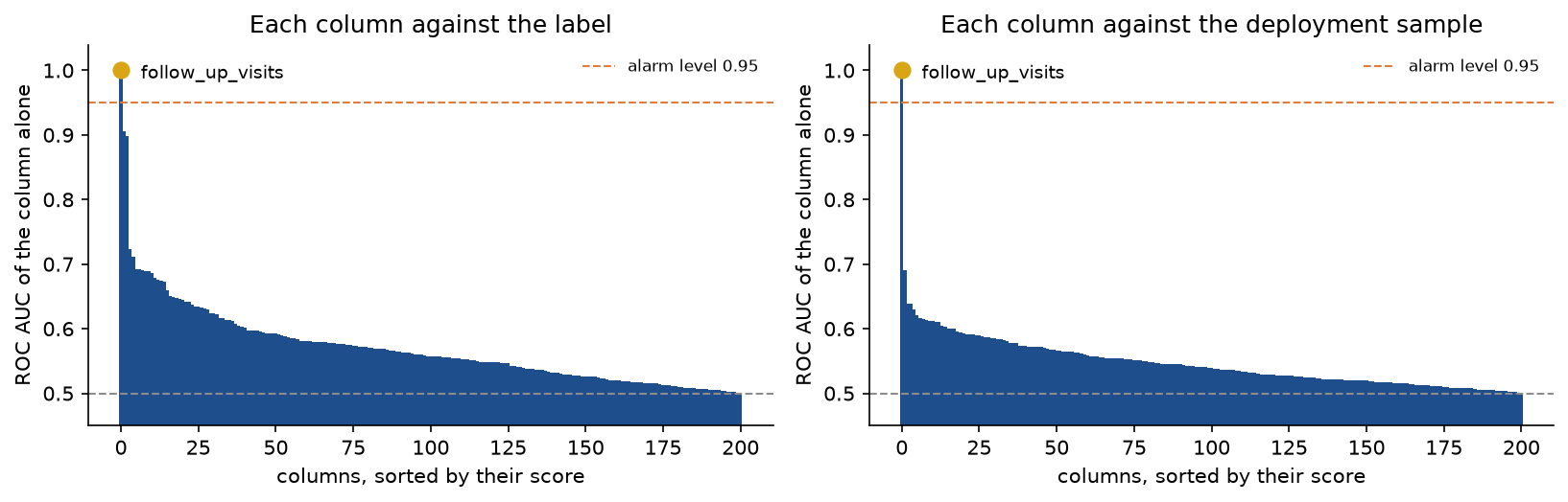
Two panels of column scores sorted from the largest, each with the alarm level 0.95 marked: against the label, follow_up_visits stands alone at 1.0 with the best measurements near 0.9; against the deployment sample, follow_up_visits again stands alone at 1.0 while every measurement stays below 0.7

These are the two column screens of the first audit. Against the label, two genuine measurements come close to the follow-up column, which is why the screen names only columns at 0.95 or with a clear lead; against the deployment sample the leak stands alone, because the column is empty at prediction time.

The notebook data_leakage_and_pitfalls.ipynb is a guided tour in the order of this page: the worked example through trace_selection and again in bare NumPy, the arithmetic and simulation of selection bias, every leak of the catalogue, the realistic run with its audit, and the same evaluations in scikit-learn. The tests in tests check the worked example and every number on this page, the mathematical properties of the metrics, splitters and steps, the audit's findings and the agreement with scikit-learn, and run in under ten seconds:

python -m pytest machine-learning/data-leakage-and-pitfalls

Every data set is synthetic, generated from a fixed seed by the package, so nothing is downloaded and no licence is involved.

In practice¶

Each pitfall below is a small, self-contained experiment from the package: the setting, the wrong pipeline, the right pipeline, both scores and the check that would have caught the leak. Scores are accuracies unless stated otherwise, computed with five-fold cross-validation or a held-out split, and where it makes sense the model is also scored on freshly generated data from the setting it will be used in.

Leaks through fitting¶

Fitting a step on all rows and then cross-validating only the model lets the test folds shape the step. How much that matters depends on how much the step learns, and from what.

Feature selection before the split. On 100 rows of pure noise, choosing the 20 features with the largest ANOVA F score among 10,000 and then cross-validating a nearest-centroid classifier gives 0.9193 on average over 30 draws (standard deviation 0.0193). Selecting inside each training fold gives 0.5047 (0.0692). The leaky score grows steadily with the number of features screened, exactly as the maximum of more noise grows; the largest of the 10,000 correlations in the first draw is 0.3993, against the rough estimate of 0.4292 from How it works.

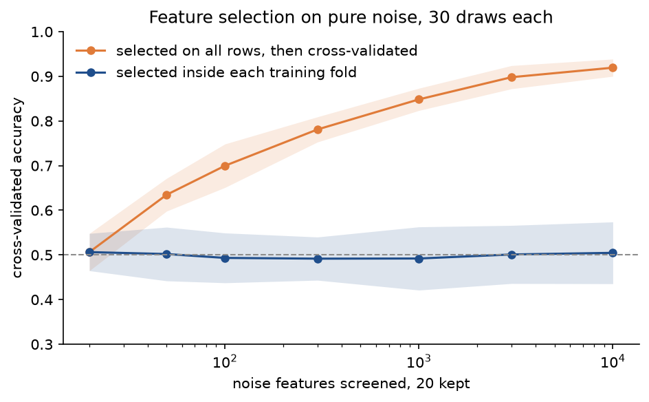
Cross-validated accuracy on pure noise against the number of noise features screened, from 20 to 10,000 on a logarithmic axis: selection on all rows climbs from 0.51 to 0.92, selection inside each fold stays near 0.5, each with a shaded band of one standard deviation

With 20 features screened and 20 kept there is nothing to choose, and the two curves coincide; every tenfold increase in the number screened adds several points of pure optimism.

PCA and scaling before the split. On 60 rows with 5 informative and 295 noise features, fitting five principal components on all rows before cross-validating gives 0.8011, against 0.7506 when the components are fitted inside each fold: an average gain of 0.0506 (standard deviation 0.0531), positive in 80 % of the 30 draws. PCA sees no labels, but with more features than rows the components bend towards the test rows, which then sit closer to the training data than new rows would. On 100 rows of ten features on wildly different scales, a scaler fitted on all rows gives 0.7607 and a scaler fitted inside each fold 0.7637: an average difference of -0.0030 (standard deviation 0.0155), with no consistent sign. Two means and two standard deviations per feature carry almost nothing about any particular test row.

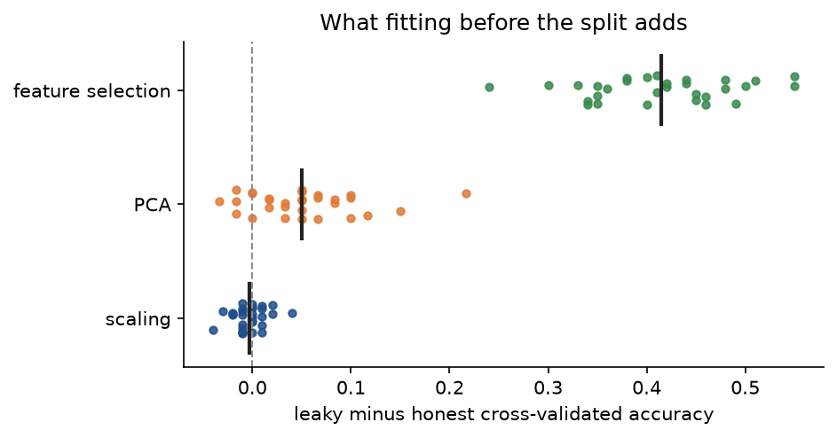
Leaky minus honest accuracy in 30 draws each: for scaling the points scatter around zero, for PCA they centre near 0.05, and for feature selection among 10,000 noise features they lie between 0.24 and 0.55, centred near 0.41

For feature selection among 10,000 features the leaky score exceeds the honest one by 0.4147 on average (standard deviation 0.0720), and in every draw. So the leak is large for steps that look at labels (selection, target encoding, any supervised feature construction), moderate for unsupervised steps with many parameters relative to the data (PCA, embeddings, clustering features on small samples), and negligible for simple scalers on large data. The rule does not depend on the size: put every fitted step inside the pipeline, because a negligible leak today becomes a large one when someone adds a step, and because a test that has to argue about leak sizes is no longer a test.

Target encoding outside the pipeline. A categorical column with 200 levels, three rows per level on average, and labels that are pure noise. Replacing each level by its mean label on all 600 rows before the pipeline puts each row's own label into its feature, and logistic regression scores 0.7367; with TargetMeanEncoder inside the pipeline it scores 0.5267. scikit-learn's TargetEncoder cross-fits inside fit_transform for exactly this reason.

The test set used for selection. Pure noise again: 320 rows, 40 features and 30 candidate models, each a k-nearest-neighbour classifier on three random features with k between 1 and 15. Holding out 80 rows, scoring all 30 candidates on them and keeping the best reports 0.5750, while the candidates average 0.5017 on the same rows; the winner scores 0.5110 on 2,000 fresh rows. Reporting the best mean score of an inner cross-validation, as GridSearchCV.best_score_ does, is the same mistake one level down: 0.5703. Nested cross-validation runs the whole selection inside each outer training set, with a four-fold inner loop, and scores the chosen candidate on the untouched outer fold: 0.5188. The rule: any score used to make a choice is spent. Report a score from data that played no part in any choice, either a test set opened once at the end or the outer loop of a nested cross-validation. Early stopping, threshold tuning, feature engineering by looking at test errors and repeated submissions to a public leaderboard all count as choices.

Augmentation before the split. Augmentation creates modified copies of training examples, here four jittered copies of each of 300 rows. Augmenting first and splitting afterwards puts copies of the same original on both sides: 96 % of the test rows have a sibling in training, and a 3-nearest-neighbour classifier finds it, scoring 0.9733. Splitting first and augmenting only the training rows gives 0.7333. The honest number carries a second lesson: without augmentation the same model scores 0.8133, so on this problem jitter hurts, a conclusion the leaky evaluation would have reversed. Random oversampling and synthetic minority oversampling are augmentation too and belong inside the training folds for the same reason.

Random transforms applied to the test rows. This happens easily when one data loader serves training and evaluation. A 15-nearest-neighbour classifier scores 0.8667 on the clean test rows; with random noise added to the test rows, twenty evaluations of the same fixed model give 0.8180 on average, anywhere from 0.7467 to 0.8667 (standard deviation 0.0341). Here the leak lowers the score rather than raising it: the score has become a random variable that depends on the evaluation seed, and it no longer measures the model on the data it will see. Keep evaluation deterministic, with no random transforms at test time, unless test-time augmentation is a deliberate part of the model, in which case it is applied identically in evaluation and in use.

Leaks through features¶

A proxy token that leaks the label. 1,200 synthetic product reviews are built from a shared vocabulary in which a handful of cue words lean towards one sentiment. The positive reviews were mostly collected through an in-store kiosk whose software stamps the token #kiosk into the text: 89.67 % of positive reviews carry it, against 4.17 % of negative ones. The token says how a review was collected, not what it says. A multinomial naive Bayes classifier on word counts scores 0.9100 on held-out reviews, and 0.7110 on 2,000 reviews from the channel the model will actually serve, where the token never appears. Removing the token before training gives 0.7633 on held-out reviews and 0.7350 in use: lower on paper, higher in practice, and honest in both places. The check is to score every feature on its own against the label. The token's single-feature ROC AUC is 0.9275; the best real word, dull, reaches 0.5633. Any single feature that predicts the label far better than everything else deserves an explanation before it is trusted. Real versions of this leak include emoticons left in text whose labels were derived from them, watermarks or rulers in medical images that only one class carries, and the name of the source folder baked into a file path.

Target leakage. 2,000 synthetic loan applications with income, debt ratio, years of credit history and previous late payments, and a default rate of 28.15 %. The export also contains collection_calls, the number of calls the collection team made, which is recorded after a default and is therefore almost a copy of the label. A standardized logistic regression with every column reaches a cross-validated ROC AUC of 0.9783 (accuracy 0.9470). Without the post-outcome column it reaches 0.7384 (accuracy 0.7480), which is what the bank can actually have when it decides. The single-feature screen flags it again: 0.9657 for collection_calls, at most 0.6507 for the others. The check is a question per column: would this value be known, with this content, at the moment the prediction is made? A stage or timestamp per column, compared with the time of the prediction, answers it mechanically, which is what the audit's time-order check does. A related trap runs the other way: a target defined as a formula of the inputs, such as a score computed from the very readings used to predict it, is predicted almost perfectly and teaches nothing that the formula did not already say.

Identifiers and ordering artefacts. 600 rows exported sorted by class, with the row number kept as the first column. A shuffled five-fold split and a logistic regression on all columns score 0.9833: the row number alone separates the classes, with a single-feature AUC of 1.0000 against 0.7596 for the best real feature. Dropping the identifier gives 0.7733. Identifiers, timestamps of data entry, file names and batch numbers all carry the order or the source of the data, which often follows the label. The ordering cuts both ways: the same honest pipeline evaluated with unshuffled folds on the sorted file scores 0.6817, because each test fold is dominated by one class that its training folds under-represent. Shuffle before an ordinary k-fold split, unless the order is time, in which case split by time.

Leaks through rows¶

Temporal leakage. A 600-step series made of a random walk, a seasonal wave and noise is modelled by a 5-nearest-neighbour regressor on the time index. With a random five-fold split every test point has its neighbours in time in the training set, and the mean absolute error is 0.4573: the model is filling gaps. With time_series_split, which always trains on the past and tests on the block that follows, the error is 1.8432. A final forecast of the last 120 steps from the first 480 gives 1.4829, in the range the forward-chaining estimate predicted and three times the random-split error.

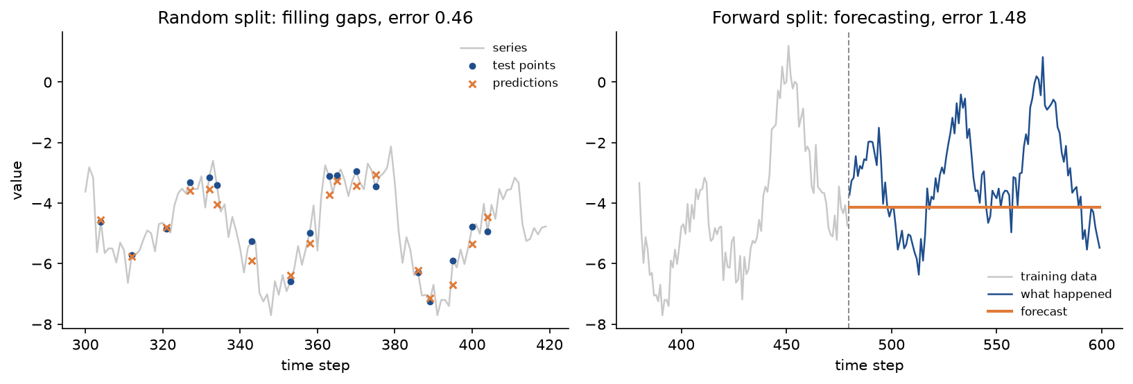
Left: a window of the series with the test points of one random fold and the model's predictions, which sit right next to the true values because their neighbours in time are in training; right: the last 100 training steps, the true continuation over the final 120 steps and a flat forecast that misses the swings

A nearest-neighbour model on the time index can only repeat the most recent values it has seen, so its forecast is flat. The random split hides that completely. Use forward-chaining splits for anything that will be used to predict the future, and leave a gap between the training and test blocks when features are built from windows that would otherwise overlap the test period.

Group leakage. 40 subjects with 10 recordings each and 12 features. Every subject has a strong personal signature, and the class, a property of the subject, shifts the features only moderately. A random five-fold split puts every subject on both sides (all 80 test rows of the first fold have their subject in training), and a 5-nearest-neighbour classifier recognises the person instead of the condition: 0.9625. group_k_fold, which keeps all recordings of a subject in the same fold, gives 0.6825, and 40 freshly generated subjects give 0.7550. The random-split estimate overshoots reality by more than 0.2; the grouped one is within the noise expected from 40 subjects. Group by whatever will be new in use: patient, speaker, device, household, store, document author.

Duplicates and near duplicates. 400 original rows, half of them repeated one to three times with a tiny jitter, as happens with reposted listings or re-exported records: 769 rows in all. Under a random five-fold split, 65.58 % of the test rows in the first fold have a near twin within distance 0.2 in training, and a 1-nearest-neighbour classifier scores 0.9181. Exact-match deduplication finds nothing to remove, because no two rows are identical. Grouping rows whose distance is below 0.2 with near_duplicate_groups recovers exactly the 400 originals; splitting by those groups gives 0.7425, close to the 0.7525 of the originals alone, with no test row left with a twin in training. Deduplicate, or group near duplicates, before splitting, with a tolerance chosen from the data: hashes of normalized text or images, rounded numeric fields, perceptual hashes for media.

Scores that answer the wrong question¶

The accuracy paradox. 3,000 rows with 2.90 % positives. On a 900-row test set with 30 positives, always predicting "negative" scores an accuracy of 0.9667 and a balanced accuracy of 0.5000. A plain logistic regression does barely better, 0.9700, but its balanced accuracy is 0.5500 and its recall 0.1000: it finds three of the thirty positives, with precision 1.0000. Weighting the classes inversely to their frequency lowers the accuracy to 0.8289 and raises the balanced accuracy to 0.7989 and the recall to 0.7667, with precision 0.1353. The ROC AUC of the two models is almost the same, 0.8824 and 0.8849, because they rank the rows almost identically and differ mainly in where they put the threshold. Report the class balance, a majority-class baseline, per-class recall and precision or a balanced metric, and choose the threshold for the costs of the application.

Distribution shift and how to detect it. Two acquisition sites. At the home site the sicker patients are scanned on a portable device whose readings are offset, so a device reading tracks the label; three genuine features carry a moderate signal. A logistic regression trained at the home site scores 0.9510 in cross-validation there and 0.5110 at a new site that uses a different device for everyone. Adversarial validation reaches a cross-validated ROC AUC of 0.9063 between home rows and new-site rows, and its largest weight by far sits on device (-2.8156, against at most 0.2999 for the others), before any new label is collected. For comparison, the two halves of the home site give 0.5418. Dropping the device reading gives 0.7610 at home and 0.7880 at the new site, and the adversarial AUC falls to 0.4600, indistinguishable from chance.

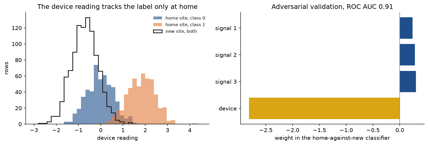
Left: histograms of the device reading at the home site, class 0 centred near 0 and class 1 near 2, and the new site's readings centred near -0.7 for both classes; right: the weights of the home-against-new classifier, small and positive for the three signals and about -2.8 for the device reading, which is highlighted

The device reading separates the classes only at home, and the adversarial classifier points straight at it. Collect a sample of the data the model will meet, compare it with the training data this way, and evaluate on a site, period or population the model has not seen whenever deployment will cross such a boundary.

All leaks at a glance¶

The catalogue, channel by channel, with the leaky estimate first and the honest one second:

Feature selection on 10,000 noise features: 0.9193 against 0.5047, where chance is 0.5.
PCA before the split: 0.8011 against 0.7506.
Scaling before the split: 0.7607 against 0.7637, no systematic gap.
Target encoding outside the pipeline, pure noise: 0.7367 against 0.5267.
The test set used to pick among 30 models, pure noise: 0.5750 against 0.5188 from nested cross-validation; the chosen model scores 0.5110 on fresh data.
Augmentation before the split: 0.9733 against 0.7333; without augmentation 0.8133.
Random transforms applied to the test rows: 0.8180 on average, from 0.7467 to 0.8667, against 0.8667 every time.
A proxy token in the text: 0.9100 against 0.7633; in use, 0.7110 for the leaky model and 0.7350 for the honest one.
A feature recorded after the outcome, in ROC AUC: 0.9783 against 0.7384.
A row identifier as a feature: 0.9833 against 0.7733.
A random split of a time series, in mean absolute error where lower is better: 0.4573 against 1.8432; the forecast of the last 120 steps scores 1.4829.
The same subject in training and test: 0.9625 against 0.6825; 40 new subjects score 0.7550.
Near duplicates on both sides: 0.9181 against 0.7425; the originals alone score 0.7525.
Accuracy under 3 % positives: an accuracy of 0.9700 against a balanced accuracy of 0.5500; the class-weighted model reaches 0.7989 balanced.
A spurious feature that changes between sites: 0.9510 against 0.7610 at the home site; at the new site 0.5110 for the leaky model and 0.7880 for the honest one.

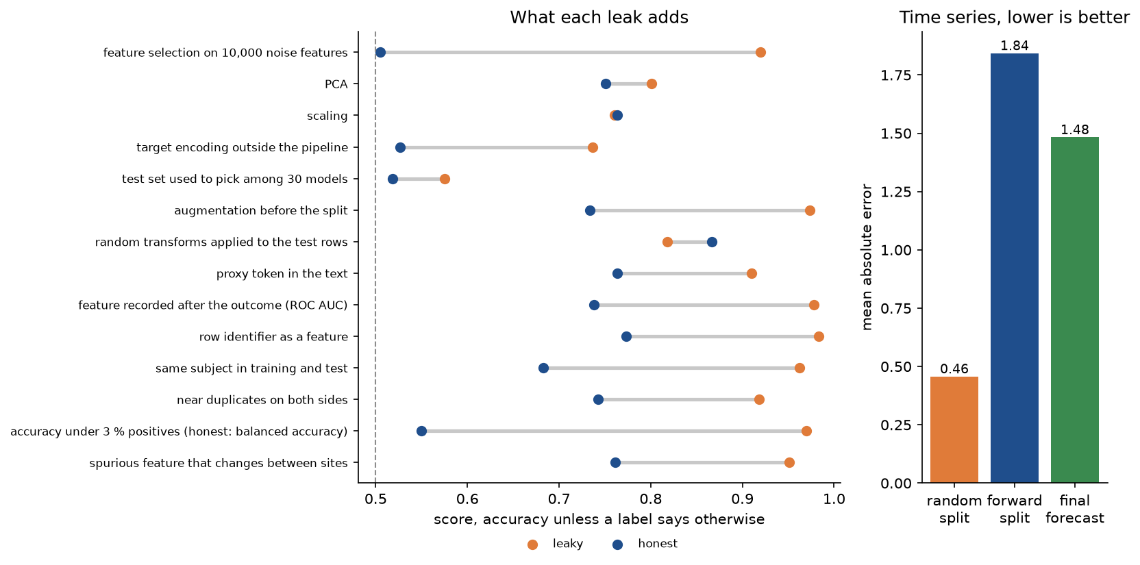
The summary makes the common shape visible: almost every leak adds between 0.15 and 0.45 to a score whose honest value is unremarkable, and the leaky numbers cluster where people stop looking for bugs.

The same in scikit-learn¶

Every piece of the package agrees with scikit-learn. The splitters return the same indices as KFold, GroupKFold and TimeSeriesSplit; the standardizer, PCA, F-score selection, target encoder, nearest centroid, nearest-neighbour models, word counts and naive Bayes agree with StandardScaler, PCA, SelectKBest(f_classif), TargetEncoder, NearestCentroid, KNeighborsClassifier, KNeighborsRegressor, CountVectorizer and MultinomialNB to within 2 × 10⁻¹³; the logistic regression agrees with LogisticRegression(C=1/penalty) to about 4 × 10⁻⁸; and roc_auc and balanced_accuracy agree with roc_auc_score and balanced_accuracy_score exactly. Fold for fold, the cross-validation scores of the catalogue's deterministic pipelines are identical in both libraries, including the nested grouped evaluation of the realistic run and the adversarial validation of the site experiment (0.906289 in both). examples/compare_with_sklearn.py prints every comparison, and tests/test_comparisons.py and tests/test_comparisons_evaluation.py assert them.

Use scikit-learn in practice: its Pipeline covers every step in the library, its splitters handle edge cases, and GridSearchCV and cross_val_score run in parallel. The package exists to make the mechanics visible, and its audit is the part worth keeping next to a scikit-learn project, because no library checks the evaluation plan for you.

The pipeline pattern¶

Most of the leaks above disappear when the whole procedure is one estimator that is fitted from scratch on the training side of every split. The leak-free analysis of the sample project reads, in scikit-learn:

import sklearn
from sklearn.feature_selection import SelectKBest, f_classif
from sklearn.model_selection import GridSearchCV, GroupKFold, cross_val_score
from sklearn.neighbors import KNeighborsClassifier
from sklearn.pipeline import make_pipeline
from sklearn.preprocessing import StandardScaler

pipeline = make_pipeline(StandardScaler(), SelectKBest(f_classif), KNeighborsClassifier())
grid = {"kneighborsclassifier__n_neighbors": [5, 15], "selectkbest__k": [10, 20, 50]}

with sklearn.config_context(enable_metadata_routing=True):
    search = GridSearchCV(pipeline, grid, cv=GroupKFold(5))
    scores = cross_val_score(search, features, labels, cv=GroupKFold(6), params={"groups": groups})

The pipeline confines scaling and selection to training folds; GridSearchCV makes the choice of settings part of the estimator, so the outer cross_val_score evaluates choosing as well as fitting; the grouped splitters at both levels keep each subject on one side. Metadata routing passes groups to the inner search as well as to the outer split. Without it, the inner GroupKFold receives no groups and every fit fails, which at least fails loudly. For time series, replace both splitters with TimeSeriesSplit; for ordinary independent rows, with shuffled KFold or StratifiedKFold. For the final model, fit search on all the data; scores describes the procedure that produced it. Text vectorizers, imputers, encoders, oversamplers (through imbalanced-learn's pipeline) and custom steps written as transformers all belong inside the pipeline.

A checklist¶

Write down how data will arrive in use: which unit is new (row, subject, site, period) and what is known at prediction time. An EvaluationPlan is one way to write it down.
Audit the columns: drop identifiers and anything recorded after the outcome, and screen single-feature AUCs and explain any that stand out.
Deduplicate, or group near duplicates, before splitting.
Split the way deployment samples: by group, by time with a gap if features use windows, or shuffled at random when rows are truly independent.
Lock the test set. Put every fitted step, including augmentation and resampling, inside a pipeline that is refitted on each training fold.
Tune with nested cross-validation or a separate validation set, with the same grouping in the inner loop, and report the outer score.
Keep evaluation data untouched and deterministic.
Report the class balance, a baseline and metrics suited to it, with the spread over folds.
Before deployment, compare training and new data with adversarial validation, grouped like the data, and evaluate on data from the deployment setting when possible.
Rerun the whole analysis on shuffled labels; it should score at chance. Treat any result that is much better than a strong simple baseline as a bug until proven otherwise.

Pitfalls¶

A pipeline protects only what is inside it. Imputation, outlier removal, target encoding or vocabulary building done on the full data frame before the pipeline is built leak exactly as if the pipeline did not exist. The target-encoding experiment above shows it: 0.7367 with the encoding done first on pure-noise labels, 0.5267 with the encoder inside the pipeline (target_encoding_leak).
An inner loop that ignores groups. Nested cross-validation with grouped outer folds but ordinary inner folds lets every candidate memorize subjects in the inner loop. In the realistic run every candidate then scores a perfect 1.0000 inside, the tie is broken arbitrarily, and the outer score falls to 0.5722 instead of 0.7556, while the grouped inner loop reports a believable 0.7383. The inner split must follow the same rule as the outer one, which the audit's plan check enforces (tests/test_realistic_run.py).
Adversarial validation with folds that ignore the groups. The check is itself an evaluation and leaks like one. Between the realistic cohort and 40 new subjects from the same population, folds that ignore the subjects give a ROC AUC of 0.9915, a shift that does not exist, because the classifier recognises the people it has already seen; folds grouped by subject give 0.4780. examples/score_traps.py prints both.
Trusting the adversarial classifier alone when there are many columns. In the sample project the follow-up column is empty in every deployment row, yet the classifier on all 201 columns reaches only 0.7232, because 200 noisy measurements from 76 subjects drown one clean signal. The same column on its own separates the two samples perfectly. Screen the columns one by one as well.
Treating the nested score as the score of the final model. Nested cross-validation estimates the performance of the whole procedure, including the choice of settings, and different outer folds may choose different settings. The deployed model is the procedure rerun on all the data, and its expected performance is the nested estimate.
Exact-match deduplication. Jittered, re-encoded or reformatted copies are not identical. On the duplicates data, grouping at tolerance zero leaves all 769 rows as separate groups, while tolerance 0.2 recovers the 400 originals (tests/test_diagnostics.py).
Unshuffled k-fold on a sorted file. scikit-learn's KFold does not shuffle by default. On data sorted by class the honest pipeline scores 0.6817 with contiguous folds instead of 0.7733 with shuffled ones; on data sorted by date, contiguous folds are what you want and shuffled ones leak.
Concluding from an adversarial AUC of 0.5 that nothing changed. The check sees only the distribution of the inputs. At a third site where the portable device is assigned at random, the device readings have exactly the home-site distribution but no longer track the label: the adversarial AUC is 0.4486 and the leaky model's accuracy is 0.5320. Conversely, a shift that the model does not rely on is harmless; look at the adversarial weights together with the model's own.
Comparing models on a small test set. The standard deviation of an accuracy near 0.5 on 80 rows is 0.0559. Two models a few points apart on such a set are not distinguishable, and picking the better one is selection on the test set again. Report the spread over folds, and prefer repeated or nested cross-validation for small data.
Fitting resampling or augmentation on all rows. Oversampling the minority class, synthetic minority oversampling and augmentation create near copies; done before the split, they produce the 0.9733 of the augmentation experiment. They belong in the training folds only.
Forgetting the gap in forward-chaining splits. If a feature at time t summarizes a window that reaches past t, or the target is a future value, the last training rows overlap the first test rows. time_series_split(..., gap=h) and TimeSeriesSplit(gap=h) drop the h rows before each test block.