MapReduce

Once a dataset is spread over hundreds of machines, every computation has to be cut into pieces that run where the data lies, and the pieces have to be put back together without the programmer handling messages, machine failures or slow disks. MapReduce achieves this with a single restriction: a job is written as two functions on key-value pairs, a map that turns each input record into intermediate pairs and a reduce that turns all the values of one key into output. Splitting the input, grouping by key across the network, retrying failed work and working around slow machines belong to the framework. This page explains the model and why it scales, traces word count and an inverted index through a small engine that prints every intermediate record, runs the same engine on separate worker processes and on a public-domain book, and measures what combiners, partitioners and skewed keys do to the data that crosses the network. It ends with matrix multiplication in one and in two passes, with the shuffle volume of each derived, measured and checked against NumPy. Afterwards you will be able to express a computation as map and reduce functions, decide whether a combiner is safe, predict how much data a job shuffles and how evenly its reducers are loaded, and read a Hadoop or Spark job with an eye for where it will be slow.

To run the code in this topic, install the base group, and the ml group for the comparison with pandas.

Intuition

A job reads a collection of records, each a pair (key, value). For a text file the key is usually the position of a line and the value the line itself. The program supplies two functions:

• map is called once per input record and emits any number of intermediate pairs. For word count it emits (word, 1) for every word of the line.
• reduce is called once per distinct intermediate key, with the list of all values emitted for that key anywhere in the job. For word count it emits (word, sum of the values).

Between the two, the framework groups every intermediate pair by key across the whole dataset. This step is the shuffle. The program never sees a machine, a network connection or a file split; it sees one record at a time in map and one key at a time in reduce. That restriction is what makes the model scale:

• Map calls share nothing. Each record can be processed on any machine, in any order and more than once, so the map work divides over as many machines as there are pieces of input.
• The only communication is the group-by-key, and it has a fixed shape. Every map task cuts its output into one piece per reduce task, and every reduce task collects its piece from every map task. Data moves once, all to all, at a point the framework controls and can schedule, compress and retry.
• Reduce calls for different keys share nothing either, so the reduce work divides over the reduce tasks.
• Tasks are deterministic functions of their input. The framework can therefore rerun any task after a failure, or run two copies of a slow one, without the program noticing.
• Computation moves to the data. Reading 1 TB from one disk at 200 MB per second takes 5,000 seconds, about 83 minutes; 500 disks reading their own share in parallel take 10 seconds. A map task scheduled on a machine that stores its input reads at local disk speed and sends nothing over the network until the shuffle.

The price of this simplicity is expressiveness. Every algorithm must be phrased as rounds of map, group-by-key and reduce, and an iterative algorithm such as PageRank needs one job per iteration with its state written to disk in between, the weakness later engines addressed (Distributed storage and compute).

Each map task reads one split of the input, typically one block of a file in a distributed file system. Its output is optionally shrunk by a combiner, a reduce-like function applied locally, then cut by the partition function p into one piece per reduce task and written to the map task's local disk. Each reduce task fetches its piece from every map task, merges the pieces sorted by key, calls reduce once per key and writes one output file. The orange arrows, which cross from the map side to the reduce side, are the shuffle.

How it works

Notation

The input D is a multiset of records, cut into M splits for M map tasks; the job has R reduce tasks. N is the number of intermediate records the mappers emit and K the number of distinct keys among them. The formula images write the count of key k as n with subscript k and the load of reduce task r as L with subscript r; in the text these are n(k) and L(r), and nmax is the count of the heaviest key. The partition function p sends key k to a reduce task p(k) between 0 and R - 1. The symbol ⊎ is multiset union, which keeps duplicates, and ⊕ is a binary operation on values.

Map, group by key, reduce

Let V(k) be the multiset of all values emitted with key k anywhere in the job. The output of the job is the union of what reduce makes of each key:

Word count fits this shape with a map that emits a 1 per word and a reduce that adds:

Two properties of this definition carry the whole system. First, map is applied record by record, so for any division of the input into splits the map output of the whole input is the union of the map outputs of the splits:

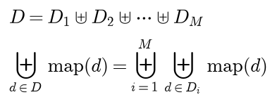
Map task i computes the i-th term without talking to any other task. Second, V(k) is a multiset: the framework promises the reducer every value of its key and nothing about their order. A correct reduce gives the same output for every order of its values. The group-by-key is the only step that needs data from all tasks.

Combiners and when they are legal

A combiner is a function with the signature of reduce that runs on one map task's output before the shuffle, so that a map task sends one partial result per key instead of every value. The framework treats it as an optimization: Hadoop may run it zero, one or several times on any subset of a key's values, once for each batch of map output it spills to disk and again when it merges the spills. A job with a combiner is only correct if that freedom cannot change the output.

A sufficient condition is that the reducer folds its values with an operation ⊕ that is associative and commutative, and that the combiner emits partial results of the same type as the map values:

Associativity lets the values be bracketed into any partial results, commutativity lets them be visited in any order, so every way of combining a multiset gives the same total, and the type condition lets a partial result be combined again or reduced like an ordinary value. Sum, maximum, minimum and set union qualify; counting is the sum of ones.

The mean does not. Suppose the values of one key are spread over m map tasks, with n(i) values of mean μ(i) in task i. The correct mean weights each task by its share of the values, but an averaging combiner followed by an averaging reducer computes the unweighted mean of the task means:

The two agree only when all the counts are equal or all the task means are equal, which is a property of the data and of the split, not of the program. The repair is to choose values that do combine: carry pairs (sum, count), combine them by adding both parts, and divide once in the reducer:

This operation is associative and commutative, and its output has the type of its input. The variance works the same way with (count, sum, sum of squares), or for numerical stability with the pairwise update of Chan, Golub and LeVeque. A median has no fixed-size summary that combines exactly; approximate quantile sketches such as t-digest are designed to merge.

When the combiner and the reducer are the same function, as in word count, the reducer must also accept its own output as input. A reducer that counts its values instead of adding them is correct while every value is a 1, and wrong as soon as a combiner has replaced several 1s by their sum.

Partitioning and load

The partition function sends key k to reduce task p(k). Hash partitioning takes a hash function h and the remainder modulo R:

Hadoop's default is (key.hashCode() & Integer.MAX_VALUE) % numReduceTasks. Range partitioning uses sorted boundaries and sends k to the number of boundaries that are at most k. Concatenating the outputs of range-partitioned reducers in order gives a globally sorted result, which is how distributed sorting works. Either way, p must be the same function on every machine and in every process, or records of one key end up at two reducers.

The load of reduce task r is the number of records whose keys it owns. Because the records of one key cannot be split, the busiest reducer receives at least the mean load and at least the heaviest key:

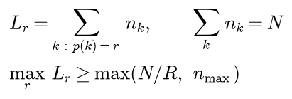
The reduce phase ends when the busiest reducer ends, so with reduce time proportional to load, its speedup over a single reducer is capped whatever R is:

How uneven is a hash partitioner below that bound? Model an ideal hash as placing every key independently and uniformly on one of the R reducers, with X(k, r) equal to 1 if key k lands on reducer r and 0 otherwise. The load is then a weighted sum of independent indicators, and its mean, variance and coefficient of variation follow line by line:

The spread depends on the data only through the sum of the squared shares n(k) / N, the probability that two randomly chosen records share a key. For K equally frequent keys the coefficient of variation is the square root of (R - 1) / K, negligible for many keys; for word frequencies, which follow Zipf's law, the few heaviest keys dominate the sum. The remedy for a hot key is to split it: append a salt from 0 to S - 1 to the key so its records spread over up to S reducers, and merge the S partial results in a second, small job.

The cost of a job

The records that cross the network are the map output after combining. Without a combiner that is every intermediate record. With a combiner that leaves one record per key, map task i sends K(i) records, the number of distinct keys in its split:

The bound shows why a combiner saves most when each map task sees many repeats of the same keys, and why it saves less as map tasks get smaller. The time of a job is roughly the map phase, divided over the machines, plus the shuffle, plus the reduce phase, and the reduce phase is set by the busiest reducer, not by the average.

Matrix multiplication in one and two passes

The product of an n by l matrix A and an l by m matrix B is a sum over the shared index j:

The input holds one record per nonzero entry, (A, (i, j, a)) or (B, (j, k, b)). Write nnz for the number of nonzero entries, c(j) for the nonzeros in column j of A and r(j) for the nonzeros in row j of B.

The diagram contrasts the two schemes derived next; the orange edges are the shuffles whose sizes the formulas count. In one pass, the mapper sends each entry of A to every output cell in its row of C and each entry of B to every cell in its column, tagged with the shared index j:

The reducer of cell (i, k) pairs the A and B values with equal j and adds their products. Every nonzero of A is copied m times and every nonzero of B n times, and each reducer holds at most 2l values:

In two passes, the first job joins on j: the mapper emits (j, (A, i, a)) and (j, (B, k, b)), and the reducer of j emits ((i, k), a b) for every pair of an A value and a B value. The second job adds the products of each cell. Its shuffle carries every product, one per pair of a nonzero in column j of A and a nonzero in row j of B:

With a combiner in the second job, each of its M map tasks sends at most one partial sum per cell of C, so the second term drops to at most M n m. For dense matrices the two-pass scheme shuffles less exactly when

which holds for all n and m from 3 up; at n = m = 2 the two are equal. The comparison is not the whole cost: the second scheme writes all its products to the distributed file system between its jobs and reads them back, pays the start-up of a second job, and gives the reducer of j an output of c(j) r(j) records from an input of c(j) + r(j). For sparse matrices the two-pass scheme wins clearly, because the one-pass scheme copies every nonzero entry across a whole row or column of C whether or not it meets a partner. Practical systems use blocks: cutting A and B into tiles and sending each tile only to the reducers that need it trades replication against reducer memory, the same tiling that makes matrix multiplication fast on a GPU.

Locality, failures and stragglers

A distributed file system stores each file as large blocks, 128 MB by default in HDFS, each replicated on three machines. The scheduler gives a map task to a machine holding a replica of its split if one is free, otherwise to a machine in the same rack, otherwise to any machine. Most map input is then read from local disks and never crosses the network.

The diagram follows one task through the two mechanisms below. The master pings every worker. When a worker stops responding, its running tasks are rescheduled elsewhere, and so are its completed map tasks, because their output lived on that worker's local disk and the reducers still need it. Completed reduce tasks are not rerun; their output is already in the distributed file system. Rerunning is safe because tasks are deterministic and commit their output atomically: a task writes to a temporary file and renames it on success, so the first attempt to finish wins and the files of every other attempt are discarded.

A phase ends when its last task ends, and one machine with a failing disk, an overloaded neighbour or a bad configuration can run several times slower than the rest. Near the end of a phase the master therefore starts backup copies of the tasks still running and takes whichever copy finishes first, which is called speculative execution. Dean and Ghemawat report that a sort took 44 % longer with backup tasks disabled. Hadoop launches a backup when a task's progress rate falls well below the average, and the LATE scheduler of Zaharia et al. instead backs up the task with the longest estimated time remaining. The cost is duplicated work, and a task that has effects outside the framework, such as writing to a database, now has them twice.

Worked example

Four short lines, numbered 0 to 3: "tea and toast", "toast and jam and tea", "jam on toast" and "milk and honey". The job is word count with M = 2 map tasks of two lines each, R = 2 reduce tasks, the summing reducer reused as the combiner, and the hash partitioner crc32(k) mod 2, where crc32 is the checksum of the word's UTF-8 bytes, zlib.crc32(b"tea") in Python.

The diagram shows the whole job at once; the steps below give every record.

Map and combine

Map task 0 reads lines 0 and 1 and emits 8 pairs: (tea, 1) (and, 1) (toast, 1) (toast, 1) (and, 1) (jam, 1) (and, 1) (tea, 1). Map task 1 reads lines 2 and 3 and emits 6: (jam, 1) (on, 1) (toast, 1) (milk, 1) (and, 1) (honey, 1).

Each map task then sorts its own output by key and sums the values of each key. Map task 0 holds "and" three times and "tea" and "toast" twice each, so its 8 records become 4: (and, 3) (jam, 1) (tea, 2) (toast, 2). Map task 1 has six different words, so its combiner only sorts them and all six records remain: (and, 1) (honey, 1) (jam, 1) (milk, 1) (on, 1) (toast, 1).

Partition, shuffle and reduce

The checksums and their remainders modulo 2 are:

• and: 133536621, reduce task 1.
• honey: 2134875284, reduce task 0.
• jam: 4125413607, reduce task 1.
• milk: 3156646934, reduce task 0.
• on: 162933192, reduce task 0.
• tea: 2391201714, reduce task 0.
• toast: 3009046592, reduce task 0.

So map task 0 sends (tea, 2) (toast, 2) to reduce task 0 and (and, 3) (jam, 1) to reduce task 1, and map task 1 sends (honey, 1) (milk, 1) (on, 1) (toast, 1) to reduce task 0 and (and, 1) (jam, 1) to reduce task 1.

Reduce task 0 receives these six records, map task 0's first. It sorts them by key and groups the values: honey [1], milk [1], on [1], tea [2], toast [2, 1]. Summing each group gives (honey, 1) (milk, 1) (on, 1) (tea, 2) (toast, 3). Reduce task 1 receives four records, groups them as and [3, 1] and jam [1, 1], and writes (and, 4) (jam, 2).

The 14 map output records became 10 shuffled records, and the reducer loads are 6 and 4. Without the combiner all 14 records are shuffled, with loads 8 and 6, and the output is the same. With only seven keys the hash puts five of them on reduce task 0; balance by hashing is a statement about many keys.

Inverted index

The same lines, now four documents. The mapper emits (word, document) for every occurrence, the combiner keeps one record per distinct (word, document) pair in its map task, and the reducer sorts the documents of each word. "and" occurs twice in document 1, so map task 0's combiner drops one record and 13 of the 14 map output records are shuffled. The postings lists are:

• and: 0, 1, 3.
• honey: 3.
• jam: 1, 2.
• milk: 3.
• on: 2.
• tea: 0, 1.
• toast: 0, 1, 2.

Set union is associative, commutative and also idempotent, so keeping distinct pairs is a legal combiner, and the reducer must still remove duplicates itself, because the combiner may not have run.

The average a combiner breaks

Now the mapper emits (first letter, word length), and the job computes the mean word length per first letter. The words starting with t are tea, with 3 letters, and toast, with 5. Map task 0 holds the t-values 3, 5, 5 and 3, and map task 1 holds the single value 5 from "jam on toast".

• Without a combiner, the reducer sees all five values and computes (3 + 5 + 5 + 3 + 5) / 5 = 21 / 5 = 4.2000.
• With the averaging reducer as the combiner, map task 0 emits 16 / 4 = 4.0000 and map task 1 emits 5 / 1 = 5.0000, and the reducer computes (4.0000 + 5.0000) / 2 = 4.5000.
• With the (sum, count) combiner, map task 0 emits (16, 4) and map task 1 emits (5, 1), and the reducer computes (16 + 5) / (4 + 1) = 4.2000.

The averaging combiner gives task 0's four words the same weight as task 1's single word. The other letters come out right by accident: every word starting with a has three letters, and h, j, m and o each have one length only.

The counting reducer fails in the same setting. Reused as the combiner it emits (and, 3) from map task 0 and (and, 1) from map task 1, and then, as the reducer, counts the two values it receives and reports (and, 2) instead of (and, 4).

Range partitioning

With the single boundary "m", keys before "m" go to reduce task 0 and the rest to reduce task 1. The output files are part 0 = (and, 4) (honey, 1) (jam, 2) and part 1 = (milk, 1) (on, 1) (tea, 2) (toast, 3); read one after the other they are sorted.

Matrix multiplication

Indices start at 0, as in NumPy. A is 2 by 3 with rows (2, 0, 1) and (-1, 3, 4); B is 3 by 3 with rows (1, 2, 0), (0, -2, 5) and (3, 1, 1). So n = 2, l = 3 and m = 3, A has 5 nonzero entries and B has 7.

One pass. Every nonzero of A goes to the m = 3 cells of its row and every nonzero of B to the n = 2 cells of its column, so the shuffle carries 5 × 3 + 7 × 2 = 29 records. The reducer of cell (1, 1) receives all of row 1 of A and column 1 of B, (A, 0, -1) (A, 1, 3) (A, 2, 4) (B, 0, 2) (B, 1, -2) (B, 2, 1), pairs them on j and computes (-1)(2) + 3(-2) + 4 × 1 = -2 - 6 + 4 = -4. The reducer of cell (0, 2) receives (A, 0, 2) (A, 2, 1) (B, 1, 5) (B, 2, 1): the zeros in row 0 of A and column 2 of B were never sent, only j = 2 appears on both sides, and C at (0, 2) is 1 × 1 = 1. All six reducers together give C with rows (5, 5, 1) and (11, -4, 19).

Two passes. The first job shuffles the 5 + 7 = 12 entries to their join keys j. The nonzeros per column of A are c = (2, 1, 2) and per row of B are r = (2, 2, 3), so the join emits 2 × 2 + 1 × 2 + 2 × 3 = 12 products, among them -2, -6 and 4 for the cell (1, 1), and the second job shuffles those 12. In total the two passes shuffle 24 records against 29 for one pass; for dense matrices of the same shapes the counts would be 2 × 2 × 3 × 3 = 36 against 6 + 9 + 18 = 33. With only three join keys, crc32 happens to send all of them to reduce task 1 of the first job.

Every number in this section is asserted by the tests in tests/test_trace.py, tests/test_engine.py, tests/test_jobs.py, tests/test_averages.py, tests/test_pitfalls.py and tests/test_matrices.py, and printed by examples/worked_word_count.py, examples/common_mistakes.py and examples/matrix_multiplication.py.

The code

The package mapreduce uses only the standard library for the engine and NumPy for the matrices, the synthetic keys and the load statistics. Matplotlib is imported inside the plotting functions and pandas inside comparisons.py, so worker processes that import the package to run tasks load neither.

• records.py holds the Record, Mapper, Reducer and Partitioner types, split_records, group_by_key and key_counts.
• partitioners.py holds stable_hash (crc32 of the key), hash_partitioner, RangePartitioner with sample_boundaries, and TablePartitioner for explicit tables.
• tasks.py holds the frozen Job (mapper, reducer, optional combiner, partitioner, number of reduce tasks, attempts allowed per task) and the two kinds of task, run_map_task and run_reduce_task, with shuffle between them. Each task returns its counts, its partitions or output, the id of the process that ran it, start and finish times and, when traced, every intermediate record.
• engine.py is the driver: run_job runs the map phase, the shuffle and the reduce phase in the calling process or on a process pool, execute_tasks retries failed attempts, and Counters and JobResult collect the outcome.
• trace.py holds the worked example's lines and format_trace, which prints a traced job in the order the data flows.
• jobs.py holds the tokenizer and the text jobs: word count, the inverted index, an index that also counts occurrences per document, and documents_with_all for Boolean queries.
• averages.py holds the three mean jobs, right and wrong; pitfalls.py holds the counting reducer and the partitioner built on Python's hash.
• skew.py holds reducer_loads, load_imbalance, the predicted and measured spread of the loads, Zipf-distributed keys and salting.
• matrices.py holds both matrix multiplication schemes and their shuffle formulas; scheduling.py holds the straggler simulation.
• datasets.py downloads and verifies the book and cuts it into lines and stories; streaming.py holds the Hadoop Streaming scripts; comparisons.py holds the pandas equivalents.
• plotting.py and load_plots.py draw every figure in the handbook's four colours.

A map task applies the mapper to every record of its split, optionally groups and combines its own output, and cuts the result into one list per reduce task:

map_output = [tuple(pair) for key, value in split for pair in job.mapper(key, value)]
combine_output = None
if job.combiner is not None:
    combine_output = [
        tuple(pair)
        for key, values in group_by_key(map_output)
        for pair in job.combiner(key, values)
    ]
partitions: list[list[Record]] = [[] for _ in range(job.reducers)]
for key, value in map_output if combine_output is None else combine_output:
    index = job.partitioner(key, job.reducers)
    partitions[index].append((key, value))

The shuffle hands reduce task r partition r of every map task, in map task order, and the reduce task sorts and groups what it receives before calling the reducer once per key:

def shuffle(map_results: Sequence[MapTaskResult], reducers: int) -> list[list[Record]]:
    return [
        [pair for result in map_results for pair in result.partitions[part]]
        for part in range(reducers)
    ]

With workers greater than one, run_job submits the map tasks to a multiprocessing pool, collects their partitions, performs the shuffle and submits the reduce tasks to the same pool. The pool uses the forkserver start method where the platform has it and spawn otherwise, so every worker is a separate interpreter that imports the package. Mappers, reducers and partitioners therefore have to be picklable: module-level functions or small frozen dataclasses such as RangePartitioner and OnePassMatrixMapper, not lambdas or functions defined in a notebook. A script that calls run_job with several workers must keep its top-level code under if __name__ == "__main__":, because each worker imports the main module. The failures argument names attempts that should raise inside the worker, for example {("map", 1): 1} for the first attempt of map task 1; the driver resubmits the task until it succeeds or the job's attempts are used up, and records the attempts in JobResult.attempts.

The examples and the project import the package, so install the repository first as described in the main README. Each example demonstrates one idea and runs in seconds from the repository root; the ones that use the book download it on first use:

• examples/worked_word_count.py prints every record of the worked example, the checksums, the run without the combiner, the inverted index and the range-partitioned output.
• examples/common_mistakes.py demonstrates the averaging combiner on the worked example and on the book, the counting reducer, Python's hash as a partitioner and map tasks too small for a combiner.
• examples/parallel_execution.py runs word count on worker processes, measures the speedup, injects failures and simulates stragglers, and saves the two figures shown under In practice.
• examples/partitioning_and_skew.py compares four partitioners on the book, sweeps the number of reducers, checks the variance formula, measures synthetic skew and salts the hot words.
• examples/matrix_multiplication.py runs both matrix schemes on the worked example, on dense matrices of growing size and on a sparse product, and checks every result against NumPy.
• examples/compare_with_libraries.py checks the engine against collections.Counter, the Hadoop Streaming scripts and pandas.

python data-at-scale/mapreduce/examples/worked_word_count.py
python data-at-scale/mapreduce/examples/common_mistakes.py
python data-at-scale/mapreduce/examples/parallel_execution.py
python data-at-scale/mapreduce/examples/partitioning_and_skew.py
python data-at-scale/mapreduce/examples/matrix_multiplication.py
python data-at-scale/mapreduce/examples/compare_with_libraries.py

The sample project, project/book_indexer.py, turns the book into a small search index on four worker processes. It runs a word count over the 9,312 non-empty lines and an inverted index over the twelve stories whose postings record how often each word occurs in each story, as (story, count) pairs whose combiner adds the counts per story. Each job runs once with and once without its combiner, which must give identical output, so the project can report what the combiner saves and how evenly the eight reduce tasks are loaded in both cases. It then checks the word count against collections.Counter, answers the word lookups given on the command line with the stories and counts of each word and the stories that contain all of them, and saves a figure. Options such as --workers, --map-tasks, --reducers and --top change the setup, and --figures sends the PNG to another folder so a custom run does not overwrite the one shown here; the default run takes a few seconds.

python data-at-scale/mapreduce/project/book_indexer.py
python data-at-scale/mapreduce/project/book_indexer.py lestrade goose --workers 8

With the defaults the project finds 105,301 words, 7,944 of them distinct, equal to collections.Counter, and an index of 7,932 terms, 288 of which occur in every story and 4,101 in only one. The combiner cuts the word count's shuffle from 105,301 records to 25,133, 76.1 % fewer, and the index's from 105,143 to 28,153, 73.2 % fewer. For the word count, the busiest of the eight reducers receives 1.44 times the mean load without the combiner and 1.09 times with it; for the index, 1.43 and 1.09. "violin" occurs 4 times in three stories (The Red-Headed League once, The Five Orange Pips twice, The Adventure of the Noble Bachelor once) and "cocaine" 3 times, once each in A Scandal in Bohemia, The Five Orange Pips and The Man with the Twisted Lip, so the only story with both is The Five Orange Pips.

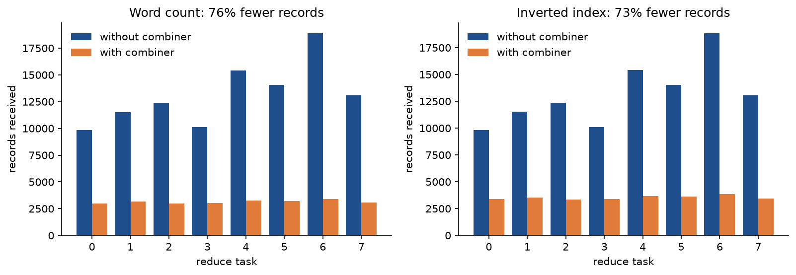
The combiner removes about three quarters of the shuffle and evens out the loads at the same time, because it collapses exactly the frequent words that made some reducers heavy: after combining, a word costs at most one record per map task however often it occurs.

The notebook mapreduce.ipynb is a guided tour in the order of this page: the worked example traced, the phases called by hand, worker processes and injected failures, the combiner rules, the partitioner that differs between processes, the book, partitioning and skew, stragglers, matrix multiplication and the comparison with Hadoop Streaming and pandas. The tests in tests check the worked example value by value, the properties above and the agreement with the reference implementations, and run in a few seconds:

python -m pytest data-at-scale/mapreduce

Data: The Adventures of Sherlock Holmes by Arthur Conan Doyle, Project Gutenberg eBook 1661, which is in the public domain in the United States. load_book downloads it on first use to .data/mapreduce/pg1661.txt at the repository root, which is not committed, removes the Project Gutenberg header and footer and checks the remaining text against a pinned SHA-256 digest, so every count on this page refers to the same edition. Readers outside the United States should check the copyright law of their country, as the Project Gutenberg terms advise. The synthetic keys, matrices and task durations are generated from fixed seeds.

In practice

The book on several processes

With workers=k, run_job runs the tasks in k separate operating-system processes. The input here is the book repeated sixteen times, 1,684,816 words, with 16 map tasks and 8 reduce tasks, and the output equals sixteen times the counts of the single book. The wall-clock times below are the best of three runs on a 16-core laptop whose other cores were partly busy, with a load average of about 2.5, so they will differ on another machine and even between runs on this one:

• 1 worker: 0.88 s, the baseline, with every task in the calling process; the mean map task takes 0.057 s.
• 2 workers: 0.82 s, a speedup of 1.07; mean map task 0.067 s.
• 4 workers: 0.61 s, a speedup of 1.45; mean map task 0.071 s.
• 8 workers: 0.61 s, a speedup of 1.44; mean map task 0.088 s.

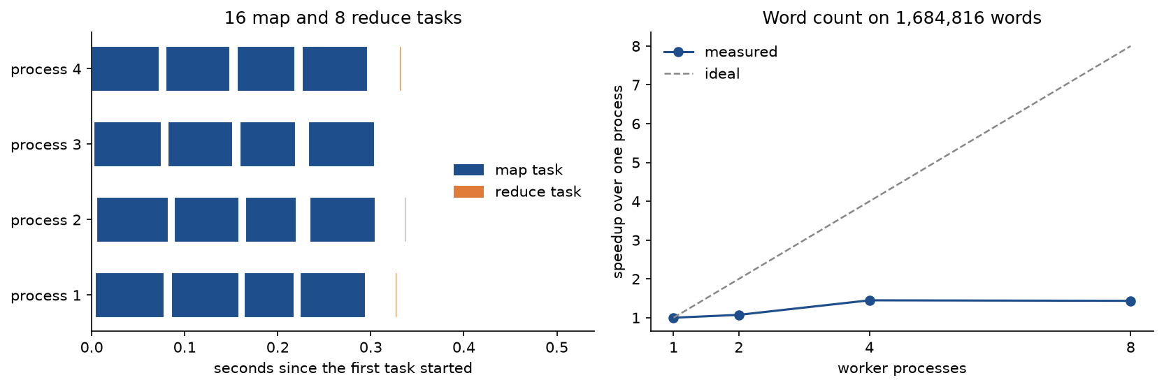
The parallelism is real, as the timeline shows, but the speedup is far from the number of workers. With two workers each map task takes 0.067 s against 0.057 s in one process, so the sixteen tasks need about 16 × 0.067 / 2 = 0.54 s, and most of the remaining 0.28 s is fixed cost: starting the processes, importing the package in each, and moving every split out of and every partition back into the one driving process, which the gap before the reduce tasks shows. That part does not shrink with more workers, which is Amdahl's law on a small scale, and it is why eight workers are no faster than four here. With more workers each task also gets slower, 0.088 s instead of 0.057 s at eight, because the cores share caches and memory bandwidth and run at a lower clock when many of them are busy. A cluster pays the same kinds of cost on a larger scale, which is why a map task is normally given seconds to minutes of work, typically one 128 MB block, rather than a fraction of a second.

Partitioning and skew, measured

Without a combiner every word occurrence is a record, and the word frequencies make the reducer loads uneven. For 8 reduce tasks the busiest load, divided by the mean of 13,162.6, is:

• 1.44 for the crc32 hash, with loads 9858, 11529, 12363, 10123, 15416, 14043, 18895 and 13074.
• 1.55 for alphabetical ranges cut at d, g, l, o, s, t and w, with loads 20007, 8464, 20356, 10233, 10708, 7670, 17337 and 10526.
• 2.09 for ranges at the quantiles of the distinct words, with loads 16091, 5178, 7286, 20518, 16219, 5220, 7232 and 27557.
• 1.27 for ranges at the quantiles of 1,000 sampled occurrences, with loads 11728, 13996, 12845, 14312, 14043, 11253, 10437 and 16687.
• 1.09 for the crc32 hash with the combiner, with loads 2999, 3157, 3001, 3042, 3239, 3225, 3414 and 3056; the mean is then 3,141.6.

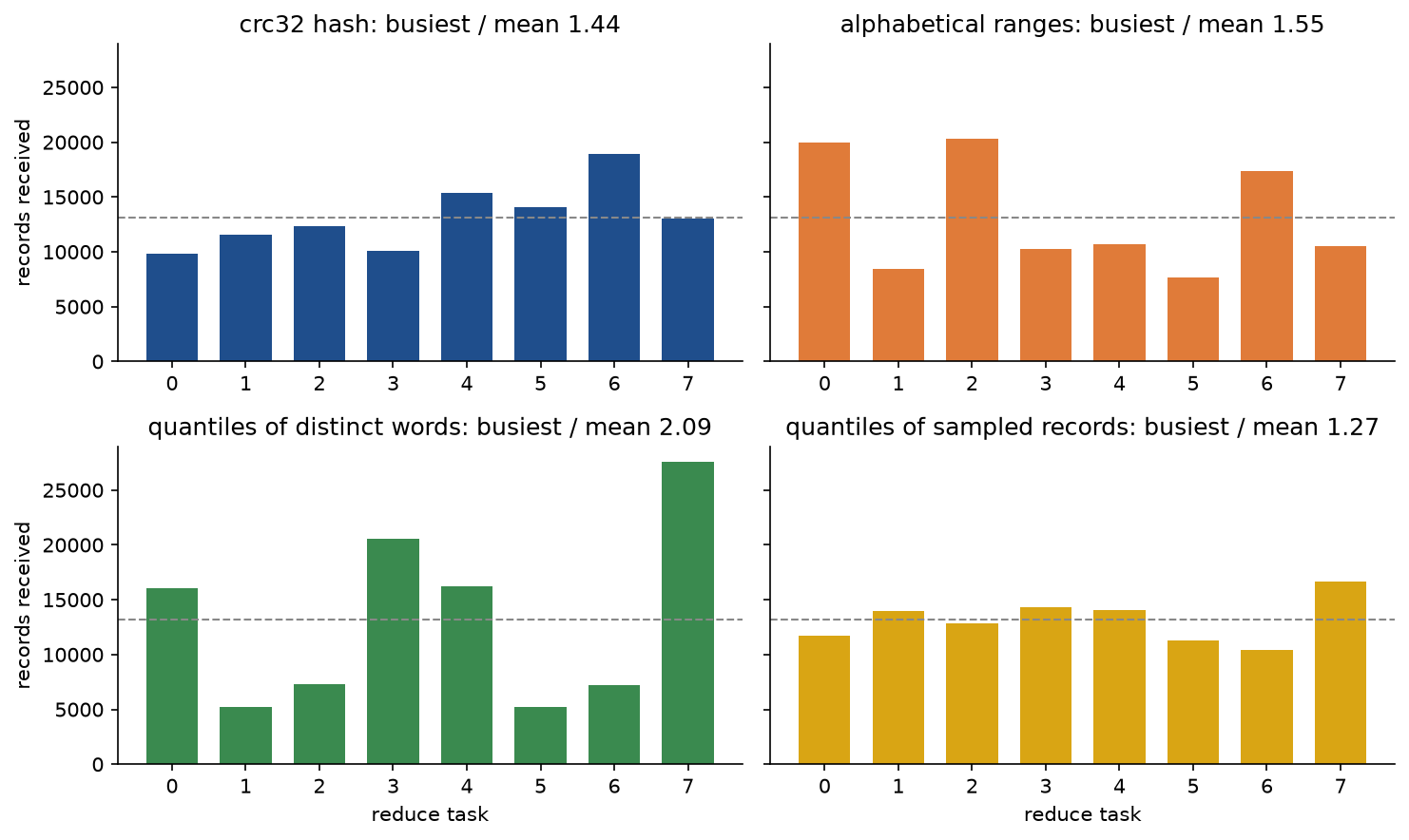
Range boundaries must be quantiles of the records, as Hadoop's total-order partitioner and Spark's range partitioner obtain them by sampling, not quantiles of the distinct keys: equal numbers of distinct words per reducer give the worst balance of all, because the reducer that owns "the", "that" and "to" also owns a full share of rare words. The sampled boundaries were banking, figure, hurry, me, probable, that and to; "the" falls between "that" and "to" and is the bulk of the busiest reducer.

Adding reduce tasks helps until the heaviest key is alone on its reducer. "the" has 5,630 of the 105,301 records, so the reduce phase can never be more than 105301 / 5630 = 18.70 times faster than a single reducer. With the crc32 hash, the busiest load and the reduce speedup over one reducer are:

• R = 2: 56,532 records, speedup 1.86; the mean load is 52,650.5.
• R = 4: 31,258, speedup 3.37.
• R = 8: 18,895, speedup 5.57.
• R = 16: 12,740, speedup 8.27.
• R = 32: 8,397, speedup 12.54; the mean load of 3,290.7 is now below the 5,630 records of "the".
• R = 64: 6,887, speedup 15.29.
• R = 128: 6,247, speedup 16.86.

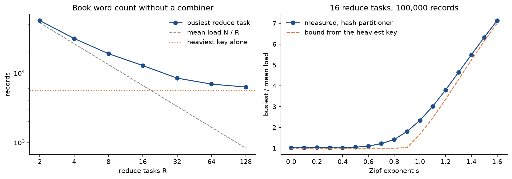
The left panel shows the ceiling at work: from 32 reducers on, the busiest load hugs the count of "the" while the mean keeps falling. The variance formula derived above predicts a coefficient of variation of the loads of 0.2570 for R = 8 and 0.5409 for R = 32. Averaged over 2,000 random placements of the keys the measured values are 0.2561 and 0.5400; the crc32 partitioner, one particular placement, gives 0.2118 and 0.5011. On synthetic keys, 100,000 records from 10,000 keys with Zipf exponent s hashed to 16 reducers, the busiest-to-mean ratio is 1.03 at s = 0, 1.05 at s = 0.5, 2.33 at s = 1 and 6.33 at s = 1.5, close to the bound 16 nmax / N once the heaviest key dominates.

Salting the eight most frequent words of the book with eight salts each brings the busiest of 32 reducers down from 8,397 records to 5,296, a busiest-to-mean ratio of 1.61 instead of 2.55. The second job that merges the salted partial counts shuffles 7,969 records and reproduces the original counts exactly.

Stragglers

simulate_schedule replays a phase of 40 tasks of 8 to 12 seconds on 10 workers, one of which runs four times slower than the others. Perfectly balanced, the work would take 42.89 s. Without backups the phase takes 77.69 s: the slow worker picks up a second task near the end and everyone waits for it. With speculative execution, a worker that finds the queue empty starts a backup copy of that task, which finishes first, and the phase takes 48.87 s.

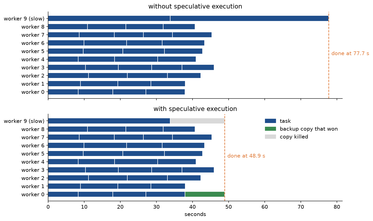
The backup costs one duplicated task and saves almost 29 seconds. Hadoop MapReduce enables speculative execution by default, while Spark leaves it off unless spark.speculation is set; either way it is safe only for tasks without side effects.

Matrix multiplication at size

For dense n by n matrices with four map tasks and four reduce tasks, every product agrees with NumPy's @ to within 7.1 × 10⁻¹⁵, and the shuffle counters match the formulas exactly. One pass shuffles 2n³ records, two passes 2n² + n³, and two passes with a combiner in the second job 2n² + 4n²:

• n = 4: 128, 96 and 96.
• n = 8: 1,024, 640 and 384.
• n = 12: 3,456, 2,016 and 864.
• n = 16: 8,192, 4,608 and 1,536.
• n = 24: 27,648, 14,976 and 3,456.
• n = 32: 65,536, 34,816 and 6,144.

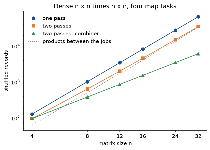
The two-pass line runs just above the dotted line of the n³ products written between its jobs, the cost the shuffle count hides. For a 60 by 40 times 40 by 50 product with 5 % of the entries nonzero, 120 in each matrix, the one-pass scheme shuffles 13,200 records and the two-pass scheme 584.

Hadoop Streaming, PySpark and pandas

Hadoop Streaming runs any executable as mapper or reducer: records arrive on standard input, key-value pairs leave on standard output as tab-separated lines, and the framework sorts the mapper output by key before the reducer reads it. The reducer therefore sees all lines of one key next to each other and only has to notice when the key changes:

import re
import sys

for line in sys.stdin:
    line = line.lower().replace("\u2018", "'").replace("\u2019", "'")
    for word in re.findall(r"[a-z]+(?:'[a-z]+)*", line):
        print(f"{word}\t1")

import sys

current, total = None, 0
for line in sys.stdin:
    word, count = line.rstrip("\n").split("\t")
    if word != current:
        if current is not None:
            print(f"{current}\t{total}")
        current, total = word, 0
    total += int(count)
if current is not None:
    print(f"{current}\t{total}")

Saved as mapper.py and reducer.py, they run on a cluster with

mapred streaming \
    -files mapper.py,reducer.py \
    -input /books/pg1661.txt -output /out/word-count \
    -mapper "python3 mapper.py" -combiner "python3 reducer.py" -reducer "python3 reducer.py" \
    -numReduceTasks 8

and locally, the usual test before a cluster run, with cat pg1661.txt | python3 mapper.py | sort | python3 reducer.py. run_streaming_locally performs that local pipeline on the whole book and gets exactly the engine's counts. The reducer can serve as the combiner because its output has the same form as its input.

In PySpark the same job is a chain of transformations. reduceByKey combines on the map side automatically, so it plays the roles of both combiner and reducer:

from operator import add

from pyspark.sql import SparkSession

from mapreduce import tokenize

spark = SparkSession.builder.master("local[4]").appName("word-count").getOrCreate()
counts = (
    spark.sparkContext.textFile(".data/mapreduce/pg1661.txt")
    .flatMap(tokenize)
    .map(lambda word: (word, 1))
    .reduceByKey(add, numPartitions=8)
)
counts.takeOrdered(10, key=lambda pair: -pair[1])

The DataFrame equivalent, spark.read.text(path) followed by splitting, explode and groupBy("word").count(), is planned by Spark SQL with a partial aggregation before the shuffle, the same idea as a combiner. The excerpt reads the raw file, header and footer included, so its counts differ slightly from the engine's; it is not run by the tests, and the data dependency group installs PySpark for readers who want to try it.

On a single machine the group-by needs no framework at all. pandas_word_counts is one call to value_counts, and pandas_postings builds the inverted index with groupby("word")["story"].unique(); examples/compare_with_libraries.py and the tests confirm that both give exactly the engine's word counts and postings.

When to use which:

• The engine here is for learning and for testing job logic: on a small input every record is visible, and the same job runs on worker processes unchanged.
• Hadoop MapReduce still runs many established batch pipelines on HDFS, but new work rarely starts there; each job writes its output to disk, which makes iterative algorithms slow.
• Spark, Flink, Beam and Dask are the usual choice for distributed batch processing today. They keep the map, shuffle and reduce structure, known in Spark as narrow and wide dependencies, and add in-memory reuse between steps, SQL and streaming.
• If the data fits on one machine's disk, a single process with pandas, DuckDB, Polars or even sort | uniq -c is often faster than any cluster, because it pays no shuffle and no task start-up.

Pitfalls

• Combining averages. A mean of means weights every map task equally instead of every value. In the worked example the averaging combiner gives 4.5000 instead of 4.2000; on the book, with 16 map tasks, the mean length of words starting with j comes out as 4.8893 instead of 4.7899. Frequent letters hardly move, which makes the bug easy to miss on a quick check. Carry (sum, count) and divide only in the reducer (tests/test_averages.py, examples/common_mistakes.py).
• Reusing a reducer that is not a fold of its values. A reducer that counts the values it receives, or that changes the type of the value, is wrong as a combiner even though it is right as a reducer: the worked example reports (and, 2) instead of (and, 4) (tests/test_pitfalls.py). Combiner output must have the type of map output and must give the same result when combined again.
• Assuming the combiner runs. The combiner is an optimization the framework may skip or apply several times. Logic that only the combiner performs, such as removing duplicates in the inverted index, must be repeated in the reducer, as postings_reducer does.
• A partitioner that differs between processes. Python randomizes hash for strings in each interpreter unless PYTHONHASHSEED is fixed. Two map tasks partitioning with hash(word) % 2 under seeds 1 and 2 send "jam" and "toast" to different reducers (with CPython 3.12; other versions may hash differently but fail the same way), and the job writes both words twice with partial counts, without any error (examples/common_mistakes.py, notebook section "A partitioner that differs between processes"). The same happens with Java arrays and enums, whose hash codes are object identities; Spark refuses array keys in a hash partitioner, and PySpark refuses to hash strings unless PYTHONHASHSEED is set. Use a hash of the key's bytes, such as crc32 here.
• Hot keys. All records of a key go to one reducer, so the reduce phase can never be faster than N / nmax times a single reducer, 18.70 for the book, and adding reducers beyond that point only adds idle tasks. Use a combiner when the aggregate allows one, otherwise salt the hot keys and merge in a second job.
• Range boundaries taken from distinct keys. Cutting the key space so that each reducer gets the same number of distinct keys ignores how often each key occurs: 2.09 times the mean load on the book against 1.27 with boundaries sampled from the records.
• Relying on the order of a key's values. The framework guarantees that a reducer gets all values of its key, not their order, which depends on which map tasks finish first. Our engine always delivers them in map task order, which can hide such a bug in tests. When order matters, put the sort field into the key, the pattern known as secondary sort.
• Side effects in map or reduce. Retried and speculative attempts run a task more than once, so a mapper that writes to a database or sends a message does so twice. Write only through the framework's output, which commits one attempt atomically, or make external writes idempotent.
• Collecting all values of a key in memory. Hadoop hands the reducer an iterator so that a hot key's values can stream from disk; turning it into a list, or calling Spark's groupByKey where reduceByKey would do, can exhaust a worker's memory on exactly the keys that matter. Our engine passes lists for readability.
• Tasks that are too small. Each task costs start-up time, and a combiner can only merge repeats within one task. With 16 map tasks the book's shuffle shrinks by 76.1 %; with 1,000 map tasks most words appear once per task and it shrinks by only 29.0 %, to 74,797 records (examples/common_mistakes.py).
• Measuring speedup on a busy machine. Worker processes compete for cores with everything else running, and the serial parts of a job, here distributing the splits and collecting the partitions in one process, do not shrink with more workers. During one run on the laptop used for this page, with other jobs occupying several cores, two workers were no faster than one process. Report the best of several runs and the load of the machine, and look at the task timeline before trusting a speedup figure (examples/parallel_execution.py).

Further reading

• J. Dean and S. Ghemawat, "MapReduce: Simplified Data Processing on Large Clusters", OSDI 2004; revised in Communications of the ACM 51(1), 107-113, 2008. The original description, including locality, re-execution and backup tasks.
• S. Ghemawat, H. Gobioff and S.-T. Leung, "The Google File System", SOSP 2003. The storage layer that makes data locality possible.
• J. Lin and C. Dyer, Data-Intensive Text Processing with MapReduce, Morgan and Claypool, 2010. Combiners, in-mapper combining, secondary sort and inverted indexing in depth.
• J. Leskovec, A. Rajaraman and J. D. Ullman, Mining of Massive Datasets, third edition, chapter 2, Cambridge University Press, 2020. Communication cost, matrix multiplication in one and two steps, and the trade-off between replication and reducer size.
• T. White, Hadoop: The Definitive Guide, fourth edition, O'Reilly, 2015. Partitioners, combiners, spills and Hadoop Streaming as implemented.
• M. Zaharia, A. Konwinski, A. D. Joseph, R. Katz and I. Stoica, "Improving MapReduce Performance in Heterogeneous Environments", OSDI 2008. The LATE scheduler for speculative execution.
• Y. Kwon, M. Balazinska, B. Howe and J. Rolia, "SkewTune: Mitigating Skew in MapReduce Applications", SIGMOD 2012.
• M. Zaharia, M. Chowdhury, T. Das, A. Dave, J. Ma, M. McCauley, M. J. Franklin, S. Shenker and I. Stoica, "Resilient Distributed Datasets: A Fault-Tolerant Abstraction for In-Memory Cluster Computing", NSDI 2012. The design that kept the shuffle and removed the disk round trip between jobs.
• T. F. Chan, G. H. Golub and R. J. LeVeque, "Algorithms for Computing the Sample Variance: Analysis and Recommendations", The American Statistician 37(3), 242-247, 1983. Mergeable variance, the combiner-friendly form of a second moment.