Probability and statistics¶

Every model in this handbook makes predictions under uncertainty and is judged on a finite, noisy sample, so two questions come up again and again. Given a model of how data arise, what data should we expect? And given the data we actually have, what can we say about the model? Probability answers the first and statistics the second. This page builds both from the axioms: events and conditional probability, Bayes' rule on a screening test where a positive result still means the condition is unlikely, random variables and six common distributions, the law of large numbers and the central limit theorem, maximum likelihood and MAP estimation, the bias and variance of estimators, confidence intervals and the bootstrap, hypothesis tests and their correction for multiple testing, and one-way ANOVA. Every formula is derived, every worked number can be checked by hand, every function is implemented from scratch in NumPy and checked against scipy.stats, and a sample project runs an A/B test from its sample size to its report. Afterwards you will be able to compute posteriors, estimates, intervals and p-values yourself, choose the right test for a comparison, plan and analyse an experiment, and recognise the misreadings that make published numbers wrong.

To run the code in this topic, install the base group, and the ml group for the comparisons with SciPy, the iris data and one pandas example.

Intuition¶

Probability starts from a model and reasons forward to data. If a die is fair, how often will two dice sum to nine? If a screening test has a known error rate, what fraction of positive results are correct? Statistics runs the other way. Having seen five thermometer readings, what is the thermometer's bias, how precisely do we know it, and is it plausibly zero? Both directions use the same rules, and two readings of what a probability means lead to the same rules: a long-run frequency of outcomes in repeated trials, or a degree of belief that is updated as evidence arrives.

The bridge between the two directions is the idea that a statistic is itself a random variable. Draw another five readings and their mean changes. The distribution of that mean over hypothetical repetitions, its sampling distribution, tells us how far a single computed mean is likely to be from the truth. The law of large numbers says the mean settles on the truth as the sample grows; the central limit theorem says the error of the mean is approximately normal with a standard deviation of σ divided by the square root of n, whatever the shape of the data. Confidence intervals, p-values and the bootstrap are all ways of using a sampling distribution.

A map of inference: a model, a distribution with parameter theta, generates data by probability; from the data, estimation gives a point estimate, and repeating the experiment in theory or by resampling gives the sampling distribution of a statistic, which yields confidence intervals, the bootstrap and p-values

The blue arrow is probability, from a model to the data it predicts. The orange arrows are statistics: a point estimate comes straight from the data, while intervals and tests need the sampling distribution, the answer to "what if we ran the experiment again?".

The other recurring idea is that conditional probabilities are not symmetric. The probability of a positive test given the condition is a property of the test; the probability of the condition given a positive test also depends on how common the condition is. Most famous mistakes in statistics, from base-rate neglect to reading a p-value as the probability that a hypothesis is false, confuse the two.

Later pages lean on this one throughout. Information theory builds entropy and cross-entropy on these distributions, calculus and optimization supplies the maximization behind maximum likelihood, naive Bayes turns Bayes' rule into a classifier, evaluation metrics applies sensitivity and specificity to classifiers, data leakage and pitfalls shows how choosing on a test set creates the same optimism as uncorrected multiple testing, and honest evaluation returns to reporting only what was measured.

How it works¶

Notation¶

The formula images use the usual symbols, and the prose names them in words with a plain symbol where it helps.

The sample space Ω is the set of all outcomes of an experiment; events A, B and H are subsets of it, and A to the power c is the complement of A.
P(A) is the probability of A and P(A | B) the probability of A given B.
X and Y are random variables, with mass function p, density f and distribution function F.
The double-struck E is the expectation; Var, Cov and ρ are the variance, covariance and correlation.
μ and σ² are the mean and variance of the population the data come from; x1 to xn is a sample of size n, usually of independent draws.
The sample mean is written x̄ and the sample variance s², with divisor n - 1; s is the sample standard deviation.
θ is a parameter and θ with a hat an estimator of it; L and ℓ are the likelihood and the log-likelihood.
Φ is the standard normal distribution function. Its q quantile, the value at which Φ equals q, is written z with subscript q in the formulas; the t quantiles are written the same way with the degrees of freedom ν added.
H0 and H1 are the null and alternative hypotheses and α is the significance level.

Sample spaces, events and the axioms¶

An experiment has a sample space of outcomes, and an event is a set of outcomes. A probability assigns a number to every event and satisfies Kolmogorov's three axioms:

Kolmogorov's axioms: the probability of every event is at least zero, the probability of the whole sample space is one, and the probability of a union of pairwise disjoint events is the sum of their probabilities

Everything else follows. A and its complement are disjoint with union Ω, so their probabilities add up to one. If A is contained in B then B is the disjoint union of A and of B without A, so P(B) is at least P(A). For any two events, the union of A and B is the disjoint union of A and of B without A, while B itself is the disjoint union of A ∩ B and of B without A; subtracting the two equations gives inclusion-exclusion. Since P(A ∩ B) is never negative, it also gives the union bound, which reappears as the Bonferroni correction:

Consequences of the axioms: the complement has probability one minus P of A, the empty set has probability zero, a subset has at most the probability of its superset, inclusion-exclusion says P of A union B is P of A plus P of B minus P of A intersect B, and the union bound says the probability of a union of m events is at most the sum of their probabilities

When the sample space is finite and all outcomes are equally likely, the probability of an event is the number of outcomes in it divided by the number of outcomes: probability becomes counting, which is what event_probability does with exact fractions.

Conditional probability and independence¶

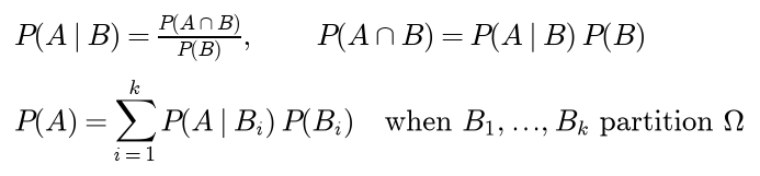
Knowing that B occurred shrinks the sample space to B and rescales it. That gives the conditional probability, for P(B) above zero, and rearranged, the product rule. If B1 to Bk partition the sample space, A is the disjoint union of its pieces inside each Bi, and the law of total probability follows:

The conditional probability of A given B is P of A intersect B over P of B; the product rule says P of A intersect B is P of A given B times P of B; the law of total probability says P of A is the sum over i of P of A given B i times P of B i when the events B i partition the sample space

A and B are independent when the probability of both is the product of their probabilities, which is the same as saying that learning B does not change the probability of A. Conditional independence given C is the same property inside C:

Independence: P of A intersect B equals P of A times P of B, which is equivalent to P of A given B equal to P of A; conditional independence given C: P of A intersect B given C equals P of A given C times P of B given C

Independence is a numerical property, not a claim about physical separation, and it is not the same as being mutually exclusive. Two mutually exclusive events of positive probability are never independent, because the probability of both is zero while the product of their probabilities is not: learning one tells you the other did not happen. Conditional independence neither implies nor follows from independence; it is exactly the assumption that naive Bayes makes about features given the class.

Bayes' rule¶

Writing the product rule both ways, P(H | E) P(E) = P(E ∩ H) = P(E | H) P(H), and dividing by P(E) gives Bayes' rule. With the law of total probability over H and its complement in the denominator:

Bayes' rule: P of H given E equals P of E given H times P of H, divided by P of E given H times P of H plus P of E given not H times P of not H

P(H) is the prior, P(E | H) the likelihood and P(H | E) the posterior. Dividing the rule for H by the rule for its complement removes the denominator and gives the odds form:

The odds form of Bayes' rule: the posterior odds of H equal the likelihood ratio of the evidence times the prior odds of H

For a screening test, let D be the condition and its prevalence the prior. The sensitivity is the probability of a positive result given the condition, and the specificity the probability of a negative result without it. A positive result multiplies the odds of the condition by the positive likelihood ratio, a negative result by the negative one:

The positive likelihood ratio is the sensitivity divided by one minus the specificity; the negative likelihood ratio is one minus the sensitivity divided by the specificity

If two results are conditionally independent given the true status, the second multiplies the odds again: the posterior after one piece of evidence is the prior for the next. The posterior depends on the prior as much as on the test, which is the base-rate effect of the worked example.

Random variables and their distributions¶

A random variable turns outcomes into numbers. Its distribution function F(x) = P(X ≤ x) is non-decreasing, tends to 0 on the left and 1 on the right, and gives every interval its probability. A discrete random variable takes countably many values and has a mass function that adds up to one; a continuous one has a density whose integral over an interval is that interval's probability:

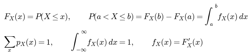
The distribution function F of x is P of X at most x; P of a less than X at most b is F of b minus F of a, which is the integral of the density from a to b; the mass function sums to one, the density integrates to one, and the density is the derivative of the distribution function

Every single value of a continuous variable then has probability zero. A density is a probability per unit length, not a probability, and can exceed one. The quantile function inverts the distribution function, and it gives a universal way to sample: if U is uniform on (0, 1), the quantile of U has distribution function F, because the quantile of u is at most x exactly when u is at most F(x):

The quantile function Q of q is the smallest x with F of x at least q; for U uniform on 0 to 1, P of Q of U at most x equals P of U at most F of x, which equals F of x

This is inverse transform sampling, and the package's samplers for the discrete distributions, the uniform and the exponential use it.

Expectation, variance, covariance and correlation¶

The expectation is the probability-weighted average of the values. It is linear, with no independence needed, as summing over the joint mass function shows:

Linearity of expectation: the expectation of a X plus b Y is the sum over x and y of a x plus b y times the joint mass p of x and y, which equals a times the expectation of X plus b times the expectation of Y

The variance is the expected squared deviation from the mean μ; expanding the square gives the shortcut, and a shift does not change it while a scale enters squared:

The variance of X is the expectation of X minus mu squared, which equals the expectation of X squared minus mu squared; the variance of a X plus b is a squared times the variance of X

The covariance measures how two variables move together, and expanding the square of their sum gives the variance of a sum:

The covariance of X and Y is the expectation of X minus its mean times Y minus its mean, which equals the expectation of X Y minus the product of the means; the variance of X plus Y is the variance of X plus the variance of Y plus twice their covariance

If X and Y are independent, the joint mass function factorizes, the covariance vanishes and variances add. The converse fails: for X symmetric around zero and Y = X², the covariance is the expectation of X³ minus the expectation of X times that of X², which is zero, although Y is a function of X. The correlation divides the covariance by both standard deviations; it lies between -1 and 1 by the Cauchy-Schwarz inequality, reaches ±1 exactly when Y is a linear function of X, and measures linear association only. Pearson's r is its sample version:

The correlation rho of X and Y is their covariance divided by the product of their standard deviations; the sample correlation r is the sum of products of deviations from the sample means divided by the square root of the product of the sums of squared deviations

Correlation is not causation. Let Z, ε1 and ε2 be independent standard normal variables and build two measurements that share Z:

X is Z plus 0.6 epsilon 1 and Y is Z plus 0.6 epsilon 2, so the correlation of X and Y is the variance of Z divided by the variance of Z plus 0.6 squared, which is 1 over 1.36, or 0.7353

X has no influence on Y, yet they are correlated because both follow the common cause Z, a confounder. Setting X by an independent random mechanism, an intervention, cuts its tie to Z and the correlation drops to zero. This is why randomized experiments, such as the A/B test of the sample project, can establish causes and observational correlations alone cannot.

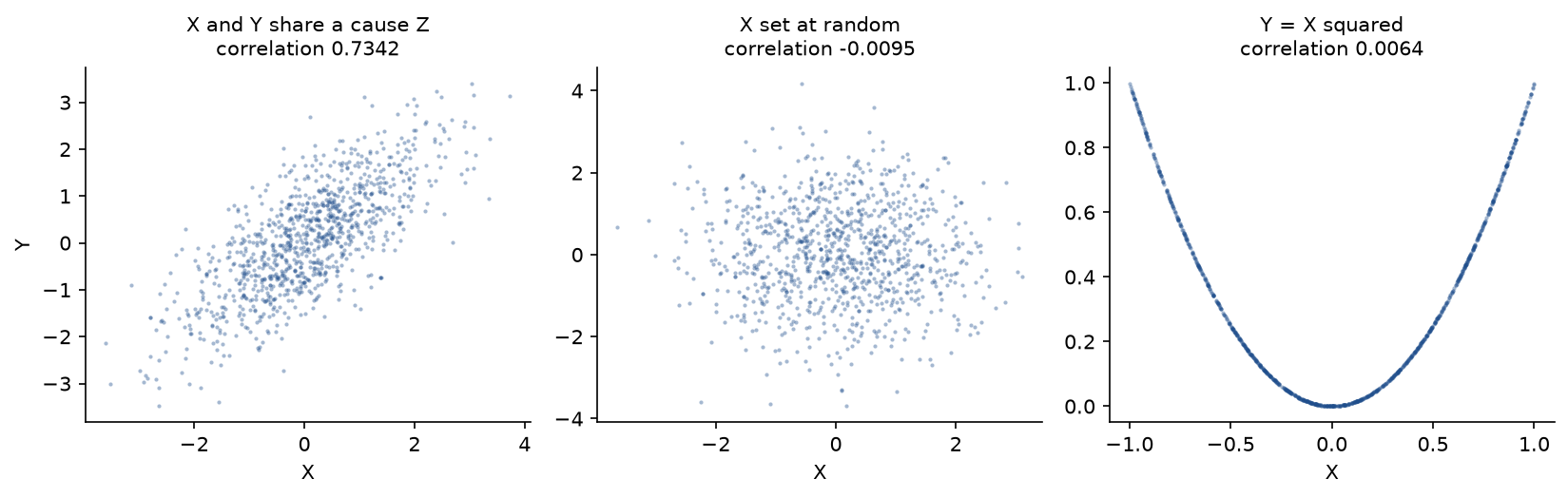
Three scatter plots of 1,000 points each: X and Y sharing a cause Z with correlation 0.7342, the same pair with X set at random with correlation -0.0095, and Y equal to X squared, a parabola, with correlation 0.0064

The correlations in the titles come from 20,000 simulated pairs. The first panel is a strong association without any causal link; the last is a perfect dependence that correlation does not see at all.

Six common distributions¶

Six distributions cover most of what later pages need. Their mass or density functions:

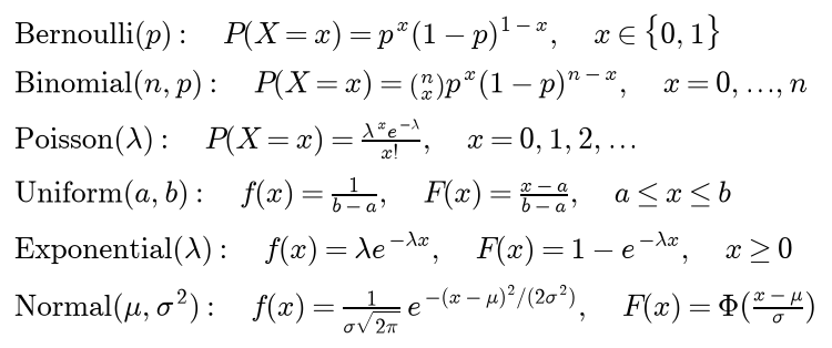
Each has a typical use. The Bernoulli distribution describes one success or failure, the binomial the number of successes in n independent trials, the Poisson counts of rare events in a fixed window, the uniform no preference within a range, the exponential waiting times between events that arrive at a constant rate, and the normal sums of many small effects such as measurement noise. Their means and variances, in that order:

Means and variances: Bernoulli p and p times one minus p; binomial n p and n p times one minus p; Poisson lambda and lambda; uniform a plus b over two and b minus a squared over twelve; exponential one over lambda and one over lambda squared; normal mu and sigma squared

They follow from the definitions.

Bernoulli: the mean is 0 times (1 - p) plus 1 times p, which is p, and since X² = X the variance is p - p², which is p(1 - p).
Binomial: a sequence with x successes in given positions has probability p to the x times (1 - p) to the n - x, and there are n choose x such sequences. The count is a sum of n independent Bernoulli variables, so by linearity the mean is np and, because independent variances add, the variance is np(1 - p).
Poisson: shifting the index of the series gives the mean, and in the same way the expectation of X(X - 1) is λ², so the variance is λ² + λ - λ² = λ. The Poisson distribution is also the limit of binomials with n trials and success probability λ/n, which is why it describes rare events:

The Poisson mean: the sum over k from one of k times lambda to the k e to the minus lambda over k factorial equals lambda times the sum over k from one of lambda to the k minus one e to the minus lambda over k minus one factorial, which is lambda

The Poisson limit: n choose k times lambda over n to the k times one minus lambda over n to the n minus k tends to lambda to the k over k factorial times e to the minus lambda as n tends to infinity

The first image shifts the index by one; the second follows because the first k factors of n choose k divided by n to the k tend to one and (1 - λ/n) to the n tends to e to the power -λ. - Uniform: integrating x over (a, b) and dividing by b - a gives the midpoint, and the second moment (a² + ab + b²)/3 gives the variance (b - a)²/12. - Exponential: one integration by parts gives the mean, another gives the second moment 2/λ² and so the variance 1/λ². The distribution is memoryless: having waited s, the chance of waiting t more is the chance of waiting t from the start.

Memorylessness is what makes the exponential the waiting time of events that arrive at a constant rate: nothing about the past changes the rate. - Normal: Z = (X - μ)/σ is standard normal, with mean 0 by symmetry and variance 1 by integration by parts, so X has mean μ and variance σ². Sums of independent normal variables are normal, with means and variances adding. About 68.27 % of the mass lies within one standard deviation of the mean, 95 % within 1.96 and 99.73 % within 3.

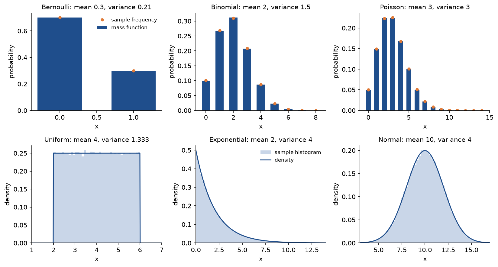
Six panels comparing the mass or density function of each distribution with 200,000 draws from the package's samplers: bars and dots for the Bernoulli, binomial and Poisson distributions, curves over histograms for the uniform, exponential and normal distributions

The sample frequencies and histograms of 200,000 draws per distribution sit on the theoretical functions, which checks the inverse transform samplers and the Box-Muller sampler of the normal distribution at a glance.

The standard normal distribution function has no closed form. The package computes it, and the distribution functions of the chi-square, t and F distributions below, from two special functions, the regularized incomplete gamma and beta functions, evaluated with their power series and continued fractions:

The regularized incomplete gamma function P of a and x is one over Gamma of a times the integral from zero to x of t to the a minus one e to the minus t; the regularized incomplete beta function I x of a and b is one over B of a and b times the integral from zero to x of t to the a minus one times one minus t to the b minus one

Substituting t = u²/2 in P(1/2, z²/2) turns the integrand into a multiple of the normal density and gives Φ:

Phi of z equals one half plus one half times the sign of z times P of one half and z squared over two

The package uses the upper half of the gamma pair for the tail, so a probability such as Φ(-9) keeps its full precision instead of being computed as one minus a number close to one.

The law of large numbers and the central limit theorem¶

Let X1 to Xn be independent with mean μ and variance σ², and let X̄ be their mean. By linearity its expectation is μ, and because independent variances add, its variance is σ²/n. Its standard deviation, σ over the square root of n, is the standard error of the mean, estimated by s over the square root of n:

The expectation of the sample mean is mu; its variance is one over n squared times n sigma squared, which is sigma squared over n; its standard error is sigma over root n, estimated by s over root n

For a non-negative Y, the expectation of Y is at least a times the probability that Y is at least a, which is Markov's inequality. Applied to the squared error of the mean it gives Chebyshev's inequality and the weak law of large numbers:

Markov's inequality: for non-negative Y, the expectation of Y is at least a times P of Y at least a; Chebyshev's inequality for the mean: P of the absolute error of the sample mean at least epsilon is at most its variance over epsilon squared, which is sigma squared over n epsilon squared and tends to zero as n grows

The central limit theorem gives the shape of the error, not just a bound. If the Xi are independent and identically distributed with finite variance, then the standardized mean converges to the standard normal distribution:

The central limit theorem: root n times the sample mean minus mu, over sigma, converges in distribution to the standard normal, so the sample mean is approximately normal with mean mu and variance sigma squared over n

The approximation improves as the skewness of the mean, the skewness of one draw divided by the square root of n, shrinks. Both theorems need their assumptions. The standard Cauchy distribution has no mean: the average of n Cauchy draws is again standard Cauchy and never settles down.

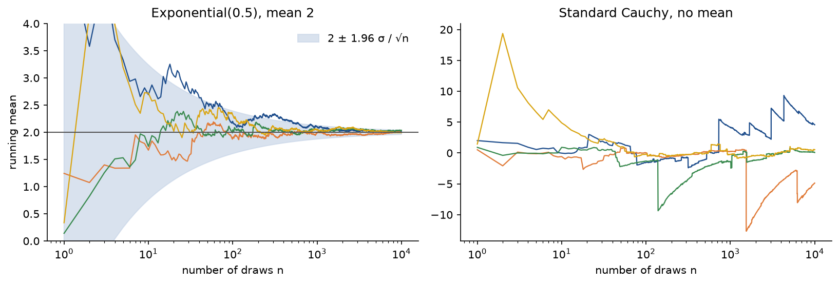
Left: running means of four sequences of exponential draws with mean 2 closing in on 2 inside the band 2 plus or minus 1.96 sigma over root n, on a logarithmic axis of n; right: running means of four standard Cauchy sequences that jump whenever a single huge draw arrives and never settle

After 10,000 draws the four exponential means lie within 0.04 of 2, while the Cauchy means end anywhere between -4.9 and 4.6. Simulation measures the rest. The interquartile range of a mean of n Cauchy draws stays near 2 for every n (1.9883 for n = 1, 1.9629 for n = 1,000), while that of the exponential mean falls from 2.2455 to 0.0869.

Chebyshev's bound is valid but loose. For means of n waiting times from the exponential distribution with mean 2, so σ² = 4, and ε = 0.5, with 20,000 simulated means per sample size, the bound, the simulated probability of missing 2 by at least 0.5 and the normal approximation are:

n = 10: bound 1.0000, simulated 0.4335, normal approximation 0.4292.
n = 25: bound 0.6400, simulated 0.2127, normal approximation 0.2113.
n = 50: bound 0.3200, simulated 0.0729, normal approximation 0.0771.
n = 100: bound 0.1600, simulated 0.0123, normal approximation 0.0124.
n = 200: bound 0.0800, simulated 0.0006, normal approximation 0.0004.

The bound holds for every distribution with that variance and is therefore far above the truth for any particular one; the central limit theorem's approximation is close from n = 25 on.

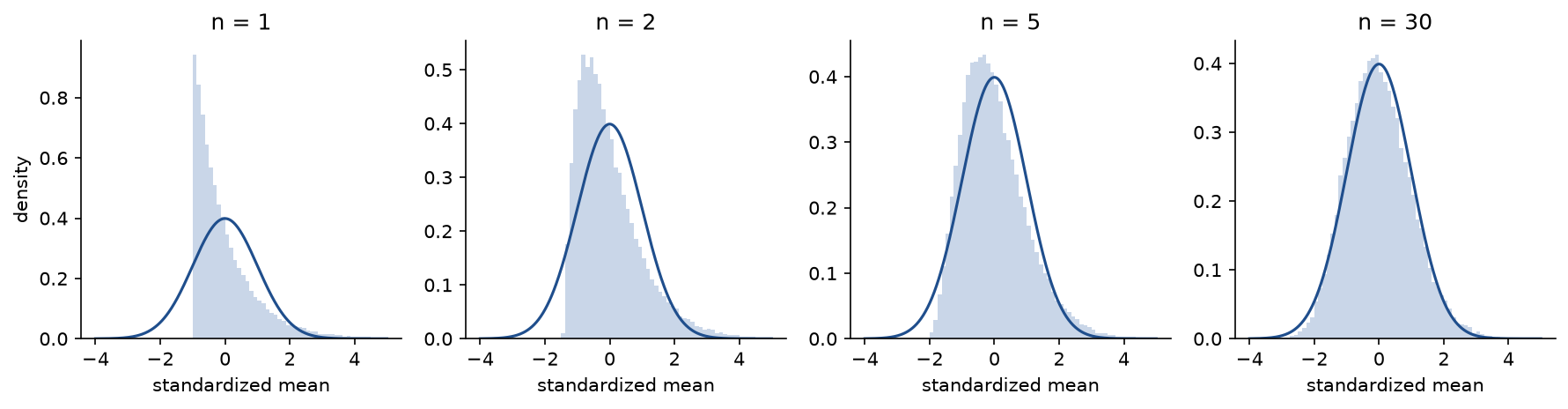
Histograms of 50,000 standardized means of exponential draws for n equal to 1, 2, 5 and 30, each against the standard normal density: the histogram is strongly skewed for n equal to 1 and nearly normal for n equal to 30

The skewness of the standardized means, 2 divided by the square root of n in theory, was 2.1040, 1.4191, 0.8863 and 0.3575 for n = 1, 2, 5 and 30, and at n = 30 the share within ±1.96 was 0.9530, close to the 0.95 of the normal distribution.

Maximum likelihood¶

For data drawn independently from a density or mass function with parameter θ, the likelihood is the probability of the observed data as a function of the parameter, and the maximum likelihood estimate maximizes it. Products of many small numbers underflow, and the logarithm turns the product into a sum without moving the maximum:

The likelihood L of theta is the product over i of f of x i given theta; the log-likelihood is its logarithm, the sum over i of the log of f of x i given theta

For k successes in n Bernoulli trials, setting the derivative of the log-likelihood to zero gives the share of successes:

The Bernoulli log-likelihood is k log p plus n minus k times log of one minus p; its derivative k over p minus n minus k over one minus p is zero when k times one minus p equals n minus k times p, so the estimate of p is k over n

The second derivative, -k/p² - (n - k)/(1 - p)², is negative, so this is a maximum. The negative log-likelihood per example is the binary cross-entropy, which is why logistic regression minimizes it. For Gaussian data both partial derivatives vanish at the sample mean and at the average squared deviation:

The Gaussian log-likelihood is minus n over two times the log of two pi sigma squared minus the sum of squared deviations from mu over two sigma squared; setting the derivative with respect to mu to zero gives the sample mean, and setting the derivative with respect to sigma squared to zero gives one over n times the sum of squared deviations from the sample mean

For a fixed variance, maximizing the Gaussian likelihood of μ is minimizing a sum of squares, so least squares in linear regression is maximum likelihood under Gaussian noise. Note the divisor n in the variance estimate, not n - 1.

MAP estimation and conjugate priors¶

A Bayesian treats θ as uncertain with a prior density, and by Bayes' rule the posterior is proportional to likelihood times prior. The maximum a posteriori estimate maximizes the log-likelihood plus the log-prior, so the prior acts as a penalty:

The posterior of theta given x is proportional to the likelihood times the prior; the MAP estimate maximizes the log-likelihood plus the log-prior

For a Bernoulli rate with a Beta(α, β) prior, the prior is proportional to p to the α - 1 times (1 - p) to the β - 1, so multiplying by the likelihood keeps the same form. A prior whose posterior stays in the same family is conjugate. The derivative used for the MLE gives the posterior mode, and the Beta mean gives the posterior mean:

The Beta prior times the Bernoulli likelihood is p to the alpha plus k minus one times one minus p to the beta plus n minus k minus one, a Beta distribution with parameters alpha plus k and beta plus n minus k; the MAP estimate is k plus alpha minus one over n plus alpha plus beta minus two, and the posterior mean is k plus alpha over n plus alpha plus beta

The prior acts like α - 1 extra successes and β - 1 extra failures. The uniform prior Beta(1, 1) gives back the MLE as its mode and Laplace's rule of succession (k + 1)/(n + 2) as its mean, the add-one smoothing that keeps a zero count from producing a probability of zero.

For a Gaussian mean with known noise σ and a Gaussian prior with mean μ0 and standard deviation σ0, the log-posterior is quadratic in μ. Setting its derivative to zero gives a precision-weighted average:

The posterior is Gaussian with precision n/σ² + 1/σ0², so its mode equals its mean. The estimate shrinks the sample mean towards the prior mean; the prior is worth σ²/σ0² observations, and its pull fades as n grows. A zero-mean Gaussian prior on the weights of a model adds a squared-norm penalty to the loss, which is L2 regularization.

Bias, variance and mean squared error¶

An estimator is a function of random data and therefore a random variable. Adding and subtracting its expectation inside the square, the cross term vanishes and the mean squared error splits in two:

The mean squared error of an estimator is the expectation of its squared error, which equals its variance plus its bias squared, where the bias is its expectation minus the true parameter

The variance estimators show the trade-off. Let SS be the sum of squared deviations from the sample mean. Since the expectation of each xi² is σ² + μ² and that of the squared sample mean is σ²/n + μ²:

SS is the sum of squared deviations from the sample mean, which is the sum of the squares minus n times the squared sample mean; its expectation is n times sigma squared plus mu squared minus n times sigma squared over n plus mu squared, which is n minus one times sigma squared

The MLE SS/n therefore has bias -σ²/n: the deviations are measured from the sample mean, which sits closer to the data than μ does. Dividing by n - 1 instead, Bessel's correction, gives the unbiased s². For normal data SS/σ² has a chi-square distribution with n - 1 degrees of freedom and variance 2(n - 1), so for the estimator SS/c:

The bias of SS over c is n minus one over c minus one, times sigma squared; its variance is two times n minus one times sigma to the fourth over c squared; its mean squared error is the variance plus the squared bias, smallest at c equal to n plus one

Setting the derivative with respect to 1/c to zero gives c = n + 1: that divisor has the smallest mean squared error, and the unbiased divisor n - 1 the largest of the three. Over 200,000 samples of five standard normal values the simulation reproduces the theory: bias 0.0012, -0.1991 and -0.3326 against 0, -0.2 and -0.3333, and mean squared error 0.5014, 0.3605 and 0.3335 against 0.5, 0.36 and 0.3333, for the divisors 4, 5 and 6. Unbiasedness is one property among several, not a guarantee of accuracy. It is also not preserved by non-linear maps: s underestimates σ on average, by a factor c4 that is 0.9400 for n = 5, and the simulated mean of s was 0.9396.

Sampling distributions: chi-square, Student's t and F¶

If Z1 to Zk are independent standard normal variables, the sum of their squares has the chi-square distribution with k degrees of freedom, mean k and variance 2k. If Z is standard normal and V is chi-square with ν degrees of freedom, independent of Z, then Z divided by the square root of V/ν has Student's t-distribution with ν degrees of freedom. A ratio of two independent chi-square variables, each divided by its degrees of freedom, has the F-distribution, and the square of a t variable is F with (1, ν) degrees of freedom.

For a normal sample, the sample mean and s² are independent and (n - 1)s²/σ² is chi-square with n - 1 degrees of freedom, hence:

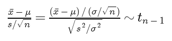
The t pivot: the sample mean minus mu over s over root n equals the standardized mean divided by the square root of s squared over sigma squared, which has a t distribution with n minus one degrees of freedom

Replacing the unknown σ by s adds the uncertainty of s, and the t-distribution has heavier tails than the normal to pay for it; it approaches the normal as the degrees of freedom grow. All three distribution functions are special functions of the previous section:

Two special cases can be checked by hand: the chi-square distribution with two degrees of freedom is exponential with mean 2, so its upper tail at x is e to the power -x/2; and since the incomplete beta function with second parameter 1 is x to the power a, the F-distribution with 2 numerator degrees of freedom has upper tail (1 + 2f/d2) to the power -d2/2.

Confidence intervals and the bootstrap¶

If σ is known, the standardized mean is standard normal whatever μ is, a pivot. It falls between the two critical values with probability 1 - α, and solving the two inequalities for μ gives the interval. With σ estimated, the t pivot gives the same form with a t quantile:

The z interval: the probability that the sample mean minus z times sigma over root n is at most mu and mu is at most the sample mean plus z times sigma over root n is one minus alpha; the t interval is the sample mean plus or minus the t quantile with n minus one degrees of freedom times s over root n

The interval is random and μ is fixed: before the data are drawn, the procedure has probability 1 - α of producing an interval that covers μ. A computed interval either contains μ or does not; the 95 % describes the method. In both forms the half-width, the margin of error, is the critical value times the standard error.

For a proportion estimated as k/n, the Wald interval plugs the estimate into the standard error and fails badly near 0 and 1; for k = 0 it has width zero. The Wilson interval instead collects every p for which the estimate lies within z standard errors computed at p itself. Squaring gives a quadratic inequality in p, and its roots are the interval:

The Wilson centre is pulled towards one half and its width never collapses, which matters near the edges. Simulation shows what the 95 % means. Over 10,000 samples of five readings from a sensor with true mean 4.0 and σ = 0.7, the t-interval covered 4.0 in a share of 0.9516 with mean width 1.6260, the z-interval with the true σ in 0.9526 with width 1.2271, and the z-interval with s in place of σ, a common shortcut, in only 0.8778 with width 1.1478.

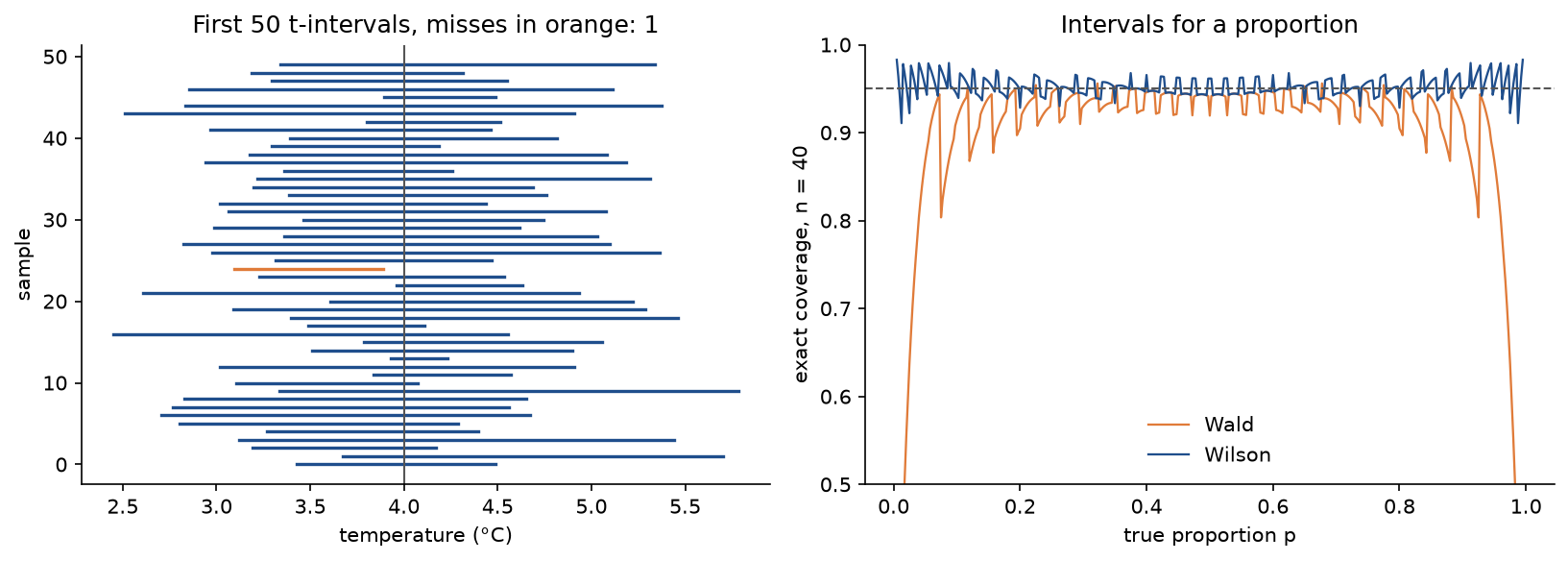
Left: the first 50 of the simulated t-intervals as horizontal segments around the true value 4.0, one of them in orange because it misses; right: the exact coverage of the Wald and Wilson intervals for a proportion with n equal to 40 against the true proportion, the Wald curve collapsing near 0 and 1 and the Wilson curve oscillating around 0.95

The coverage curves are exact, computed by adding the binomial probabilities of every count whose interval contains p. With n = 40, the Wald interval covers 0.5531 at p = 0.02, 0.8681 at p = 0.05 and only 0.9193 at p = 0.5, against 0.9543, 0.9520 and 0.9615 for the Wilson interval. For p between 0.1 and 0.9 the Wald coverage ranges from 0.8678 to 0.9559 and the Wilson coverage from 0.9283 to 0.9725; Wilson dips to 0.9108 only at the very edge of the grid, where Wald collapses. For 7 successes in 40, Wald gives (0.0572, 0.2928) and Wilson (0.0875, 0.3195).

When no formula for the standard error exists, the bootstrap estimates the sampling distribution by resampling. The plug-in principle replaces the unknown distribution by the empirical one, which puts mass 1/n on each data point. Draw B resamples of size n with replacement, compute the statistic on each, and use their spread as the spread of the statistic. The percentile interval takes the α/2 and 1 - α/2 quantiles of the resampled statistics. It works well for smooth statistics and moderate n; it fails for statistics that depend on extremes, such as the maximum, and in very small samples, where the empirical distribution is a poor stand-in. The BCa interval, SciPy's default, corrects the percentile interval for bias and skewness.

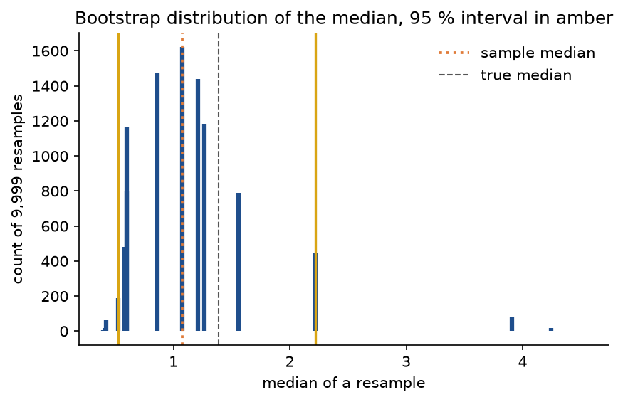
The bootstrap distribution of the median of 25 waiting times as blue spikes at a handful of values, with the 95 % percentile interval from 0.52 to 2.22 in amber, the sample median 1.08 dotted in orange and the true median 1.39 dashed in grey

Here the bootstrap gives an interval for the median of 25 exponential waiting times with mean 2: sample median 1.0788 against the true median 2 ln 2 = 1.3863, bootstrap standard error 0.5200 and 95 % percentile interval (0.5241, 2.2204). The distribution is lumpy, 17 distinct values in 9,999 resamples, because the median of a resample is always one of the data values. Over 1,000 fresh data sets the interval covered the true median in a share of 0.9460.

Hypothesis tests¶

A test compares a null hypothesis H0, such as μ = μ0, with an alternative H1. A test statistic summarizes the data, and its null distribution is its distribution when H0 holds. The p-value is the probability, computed under H0, of a statistic at least as extreme as the one observed, and the test rejects H0 at level α when p ≤ α. Rejecting a true H0 is a type I error, with probability α by construction; keeping a false H0 is a type II error, with probability β; and 1 - β is the power.

For a continuous statistic and a true H0, the p-value is uniformly distributed on (0, 1). For a one-sided test the p-value is one minus the null distribution function at the statistic, and that distribution function evaluated at its own random variable is uniform:

For a one-sided test p equals one minus F zero of T, so P of p at most u equals P of F zero of T at least one minus u, which equals u

That is why 5 % of tests of true nulls come out "significant" at the 5 % level, however large the sample. A two-sided test at level α rejects μ0 exactly when μ0 lies outside the 1 - α confidence interval built from the same pivot.

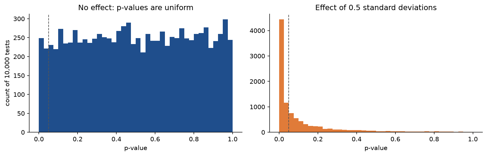
Histograms of p-values from 10,000 one-sample t-tests on samples of 20: flat between 0 and 1 when there is no effect, and piled up near zero when the true mean is half a standard deviation away

Under the null hypothesis the share of p-values below 0.05 was 0.0470; with a true effect of half a standard deviation it was 0.5597, the power of the test.

The common tests differ in their statistic and its null distribution. The one-sample tests standardize the distance of the mean from μ0, by σ when it is known and by s when it is not; the paired t-test is the one-sample t-test on the differences within pairs, with μ0 = 0:

The z statistic is the sample mean minus mu zero over sigma over root n, standard normal under H0; the t statistic is the sample mean minus mu zero over s over root n, t distributed with n minus one degrees of freedom under H0

Two independent samples are compared through the difference of their means. Student's test pools the two variances and is exact when they are equal; Welch's test keeps them apart and approximates the null distribution by a t-distribution with estimated degrees of freedom:

Two server builds with 12 and 30 runs and standard deviations of 2 and 6 give Student's t = -2.2684 with p = 0.0288 and Welch's t = -3.4003 on 36.4201 degrees of freedom with p = 0.0016. Here the larger group has the larger spread, so the pooled variance overstates the standard error and the pooled test is conservative; in the opposite arrangement it is anti-conservative, as the Pitfalls show.

Counts in categories are compared with their expected counts. In a goodness-of-fit test the expected counts are given, and the null distribution is approximately chi-square with k - 1 - m degrees of freedom when m parameters were fitted. In a test of independence on an r by c table, the share of row i and column j is estimated as the product of the row and column shares, so the expected count is the row total times the column total divided by the grand total; once the margins are fixed only (r - 1)(c - 1) cells are free:

The chi-square statistic is the sum over categories of observed minus expected squared over expected; under independence the expected count of row i and column j is the row total times the column total over the grand total, with r minus one times c minus one degrees of freedom

The chi-square approximation needs expected counts of about 5 or more in every cell. Comparing two proportions, the core of an A/B test, is the 2 by 2 case. Under H0 both groups share one rate, estimated by pooling them, and the square of the resulting z statistic is exactly the chi-square statistic of the 2 by 2 table:

The two-proportion z statistic is the difference of the two observed rates divided by the square root of the pooled rate times one minus the pooled rate times one over nA plus one over nB, where the pooled rate is the total successes over the total trials

The power of the two-sided z-test follows from its statistic under H1. With a standardized effect δ, the statistic is normal with mean δ times the square root of n and variance 1:

The power of the two-sided z-test is Phi of delta root n minus the critical value plus Phi of minus delta root n minus the critical value, with delta the difference of the means in units of sigma

For δ = 0.5, n = 20 and α = 0.05 that is 0.6088; the exact power of the t-test, from the noncentral t-distribution, is 0.5645, a little lower because σ is estimated, and the simulated 0.5597 above agrees. Solving the same equation for n plans an experiment. For two proportions pA and pB, keeping the larger term only:

The users needed per group are the square of the critical value times the square root of two p bar times one minus p bar, plus the power quantile times the square root of pA times one minus pA plus pB times one minus pB, divided by the squared difference of the two rates, where p bar is their average

The sample project uses this formula to size its A/B test before collecting any data. Choosing among the tests comes down to what the question compares:

The leaves in green are the tests this package implements, except the exact test for small counts, which SciPy provides as scipy.stats.fisher_exact.

Multiple testing¶

With m independent tests of true null hypotheses at level α, the probability of at least one false rejection, the family-wise error rate, grows quickly: 0.6415 for 20 tests at 0.05. The union bound gives the simplest remedy, testing each hypothesis at α/m:

The probability of at least one false rejection among m independent true nulls is one minus one minus alpha to the m; by the union bound, the probability of any false rejection is at most the sum of the probabilities of each, which is at most m times alpha over m, which is alpha

Three standard procedures, each written as adjusted p-values compared with α:

Bonferroni multiplies each p-value by m. It controls the family-wise error rate for any dependence between the tests.
Holm sorts the p-values and rejects step by step while the i-th smallest is at most α/(m - i + 1), stopping at the first failure. It also controls the family-wise error rate and rejects everything Bonferroni rejects, and sometimes more.
Benjamini-Hochberg finds the largest i whose sorted p-value is at most iα/m and rejects the first i. It controls the false discovery rate, the expected share of false rejections among all rejections, at the share of true nulls times α for independent tests. It accepts some false discoveries in exchange for much more power when many effects are real.

Adjusted p-values: Bonferroni, the minimum of one and m times p i; Holm, the running maximum over j up to i of the minimum of one and m minus j plus one times the j-th smallest p-value; Benjamini-Hochberg, the running minimum over j from i on of the minimum of one and m times the j-th smallest p-value over j

The running maximum in Holm's formula implements "stop at the first failure", and the running minimum in Benjamini-Hochberg's implements "reject everything up to the largest i that passes". Families of 20 t-tests on samples of 20, of which 5 have a true effect of 0.6 standard deviations, repeated 2,000 times, show the trade-off; each item gives the family-wise error rate, the mean false discovery proportion and the power:

No correction: 0.5450, 0.1527 and 0.7233.
Bonferroni: 0.0305, 0.0171 and 0.2582.
Holm: 0.0325, 0.0176 and 0.2633.
Benjamini-Hochberg: 0.1120, 0.0385 and 0.3833.

Bonferroni and Holm keep the family-wise error rate below 0.05 at a large cost in power. Benjamini-Hochberg allows an occasional false discovery, keeps their average share near 15/20 times 0.05, which is 0.0375, as the theory says, and finds half as many real effects again.

One-way ANOVA¶

Suppose k groups have nj observations each, N in total, group means x̄j and grand mean x̄. The model says each observation is an overall mean plus a group effect plus independent normal noise with variance σ², and H0 says all group effects are zero. Write each deviation from the grand mean as a within-group part plus a between-group part, square and sum; the cross term vanishes because deviations from a group's own mean sum to zero within the group:

Each deviation from the grand mean is the deviation from the group mean plus the deviation of the group mean from the grand mean; the total sum of squares equals the within-group sum of squares plus the between-group sum of squares, weighted by group sizes; SST equals SSW plus SSB, and N minus one degrees of freedom split into N minus k and k minus one

Dividing each sum of squares by its degrees of freedom gives the mean squares, and their ratio is the test statistic:

The F statistic is SSB over k minus one divided by SSW over N minus k, the ratio of the mean squares MSB over MSW, which has the F distribution with k minus one and N minus k degrees of freedom under H0; the expected MSW is sigma squared and the expected MSB is sigma squared plus the sum of n j times tau j squared over k minus one

F is near 1 when H0 holds and grows with the spread of the group means. With two groups, F equals the square of the pooled t statistic and the two tests agree exactly. ANOVA assumes independent observations, normal errors within groups and equal variances; a significant F says that some means differ, not which ones.

Worked example¶

Every number below is computed in double precision and shown to four decimals; where a sum written out from rounded terms differs in the last digit, the text says so. examples/worked_examples.py prints the results of each section, and the tests in tests assert every number, the hand-calculation steps included.

Two dice¶

Two fair dice have 36 equally likely ordered outcomes. The sum is 9 for (3, 6), (4, 5), (5, 4) and (6, 3), so the probability of a nine is 4/36 = 1/9. At least one six has probability 1 - 25/36 = 11/36 by the complement, and 1/6 + 1/6 - 1/36 = 11/36 by inclusion-exclusion. "The first die is even" (probability 1/2) and "the sum is 7" (probability 1/6) occur together for (2, 5), (4, 3) and (6, 1), probability 3/36 = 1/12, which is 1/2 times 1/6, so they are independent. "The sum is 9" and "the first die is 6" are not: given a 6 first, a nine needs a 3 second, so its probability rises from 1/9 to (1/36)/(1/6) = 1/6.

A screening test and the base rate¶

A test has sensitivity 0.96 and specificity 0.94 and is used in a population where 1.5 % have the condition. In natural frequencies for 10,000 people, 150 have the condition and 9,850 do not; the test finds 0.96 × 150 = 144 of the 150 and raises a false alarm for 0.06 × 9,850 = 591 of the others.

A natural-frequency tree: 10,000 people split into 150 with the condition and 9,850 without; the 150 split into 144 positive and 6 negative results, the 9,850 into 591 positive and 9,259 negative; the 144 and 591 positives together make 735 positive results, of which 144 have the condition, a share of 0.1959

Reading the tree from the right: 735 people test positive, 144 + 591, so the probability of a positive result is 0.0735, and of those only 144 have the condition. Bayes' rule says the same in symbols:

P of D given a positive result equals 0.96 times 0.015 over 0.96 times 0.015 plus 0.06 times 0.985, which is 0.0144 over 0.0144 plus 0.0591, which is 144 over 735, or 0.1959

Four in five positive results are false alarms, because people without the condition outnumber those with it 66 to 1 and 6 % of a large number is larger than 96 % of a small one. In odds:

The prior odds are 0.015/0.985 = 3/197 and the positive likelihood ratio is 0.96/0.06 = 16, so the posterior odds are 48/197 and the probability is 48/245 = 0.1959.
An independent second positive test multiplies the odds by 16 again, to 768/197, a probability of 768/965 = 0.7959.
A negative result has likelihood ratio 0.04/0.94 = 0.0426 and leaves a probability of 6/9,265 = 0.000648; a positive followed by a negative ends at 0.0103.

The same test gives P(D | +) = 0.0158 at a prevalence of 0.001, 0.1959 at 0.015, 0.6400 at 0.1 and 0.9412 at 0.5.

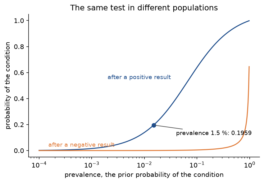
The probability of the condition after a positive result and after a negative result against the prevalence on a logarithmic axis: the positive curve rises from almost zero through 0.1959 at a prevalence of 1.5 % towards one, while the negative curve stays near zero until the prevalence is very high

Nothing about the test changes along the curves, only the population it is applied to. The figure is the reason a screening programme confirms every positive result with a second, independent test.

Six distributions at one point each¶

One value of each distribution, computed from the formulas under How it works:

Bernoulli(0.3): P(X = 1) = p = 0.3000, with mean 0.3 and variance 0.21.
Binomial(8, 0.25): P(X = 2) = 28 × 0.25² × 0.75⁶ = 1.75 × 0.1780 = 0.3115, and P(X ≤ 2) = 0.1001 + 0.2670 + 0.3115 = 0.6785, with mean 2 and variance 1.5. The three rounded terms add to 0.6786, against 0.6785 at full precision.
Poisson(3): P(X = 2) = (9/2) e⁻³ = 4.5 × 0.0498 = 0.2240, and P(X ≤ 2) = e⁻³ (1 + 3 + 4.5) = 0.4232, with mean and variance 3.
Uniform(2, 6): the density at 3 is 1/4 = 0.2500 and P(X ≤ 3) = (3 - 2)/4 = 0.2500, with mean 4 and variance 16/12 = 1.3333.
Exponential(0.5): the density at 2 is 0.5 e⁻¹ = 0.1839 and P(X ≤ 2) = 1 - e⁻¹ = 0.6321, with mean 2 and variance 4. It is memoryless: P(X > 5 | X > 3) is e to the power -2.5 divided by e to the power -1.5, which is e⁻¹ = 0.3679 = P(X > 2).
Normal(10, 2²): the density at 12 is e to the power -1/2 divided by 2√(2π), which is 0.1210, and P(X ≤ 12) = Φ(1) = 0.8413, with mean 10 and variance 4.

Estimating a pass rate: MLE and MAP¶

A component passes 13 of 20 stress runs. The MLE is 13/20 = 0.65, where the log-likelihood is 13 ln 0.65 + 7 ln 0.35 = -5.6002 - 7.3488 = -12.9489; the rounded terms add to -12.9490. With a Beta(3, 3) prior, a mild belief that the rate is near one half, the posterior is Beta(3 + 13, 3 + 7) = Beta(16, 10). Its mode, the MAP estimate, is (16 - 1)/(16 + 10 - 2) = 15/24 = 0.625, and its mean is 16/26 = 0.6154. Both are pulled from 0.65 towards the prior's 0.5. With 0 passes in 4 runs the MLE would be 0, a claim that the component can never pass; the posterior mean under the uniform prior is 1/6 = 0.1667.

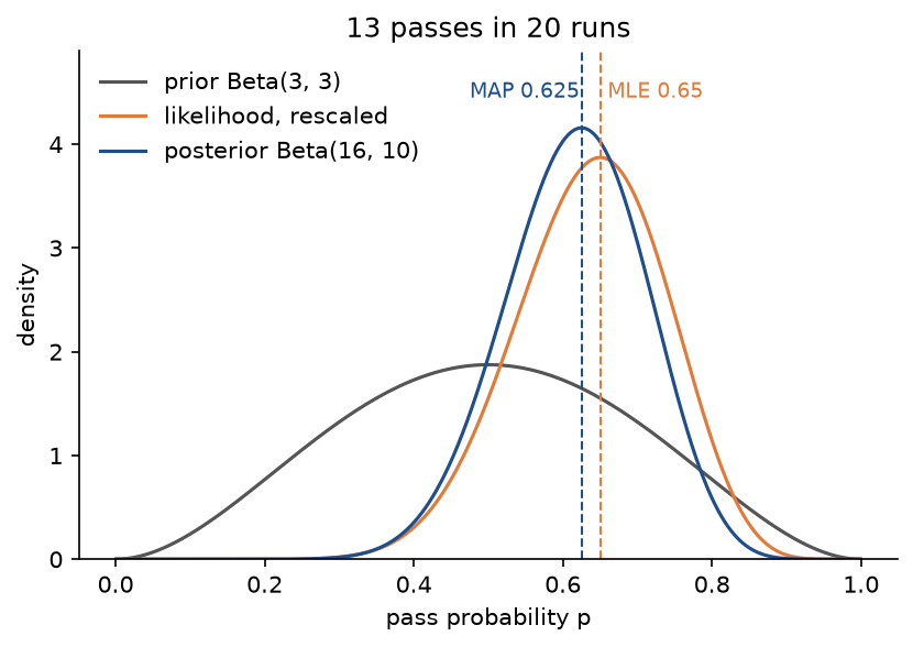
Prior Beta of 3 and 3, the likelihood rescaled to a density, and the posterior Beta of 16 and 10 for the pass probability, with the MLE 0.65 and the MAP estimate 0.625 marked by dashed lines

The posterior is narrower than both the prior and the likelihood and sits between them, closer to the likelihood because 20 runs carry more information than the prior's four pseudo-observations.

A thermometer check: estimates, an interval and two tests¶

A thermometer placed in a bath held at 4.0 °C reads 4.1, 5.3, 3.6, 4.8 and 5.2. The readings sum to 23.0, so the sample mean is 4.6. The deviations are -0.5, 0.7, -1.0, 0.2 and 0.6, their squares 0.25, 0.49, 1.00, 0.04 and 0.36, and SS = 2.14. Hence:

The MLE of the variance is 2.14/5 = 0.428, and s² = 2.14/4 = 0.535, so s = 0.7314 and the standard error is s/√5 = 0.3271.
MAP with a prior: if the maker states that the bias is small, a prior N(4.0, 0.5²), and the noise standard deviation σ = 0.7 is taken as known, the precisions are 1/0.25 = 4 for the prior and 5/0.49 = 10.2041 for the data. The MAP estimate is (4 × 4.0 + 10.2041 × 4.6)/(4 + 10.2041) = 62.9388/14.2041 = 4.4310, exactly 257/58, with posterior standard deviation 1/√14.2041 = 0.2653. The data get weight 0.7184 and the prior is worth 0.49/0.25 = 1.96 readings.
Confidence intervals: with σ estimated, the t quantile with 4 degrees of freedom is 2.7764 and the 95 % interval is 4.6 ± 2.7764 × 0.3271 = 4.6 ± 0.9082 = (3.6918, 5.5082). If σ = 0.7 is known, σ/√5 = 0.3130, z = 1.9600 and the interval is 4.6 ± 0.6136 = (3.9864, 5.2136); the rounded product 1.96 × 0.3130 is 0.6135.
Tests of H0: μ = 4.0 against μ ≠ 4.0: with σ known, z = 0.6/0.3130 = 1.9166 and p = 2(1 - Φ(1.9166)) = 0.0553. With σ estimated, t = 0.6/0.3271 = 1.8343 on 4 degrees of freedom and p = 0.1405, or 0.0703 one-sided for the alternative μ > 4.0.

Neither test is significant at 0.05, in line with both intervals containing 4.0. That is not evidence that the thermometer is accurate: the estimated bias is 0.6 °C and the t-interval allows anything from -0.31 to 1.51 °C. Five readings cannot tell. Referring the same t = 1.8343 to the normal distribution instead of the t-distribution with 4 degrees of freedom would give p = 0.0666.

Failures by sensor model: a chi-square test¶

Three sensor models were checked for readings that fail quality control. Model A failed 12 of 100 checks, model B 25 of 150 and model C 13 of 50, so 50 of the 300 readings failed. Under independence the expected counts are the row total times the column total over 300:

Model A: 100 × 50/300 = 16.6667 failures and 83.3333 passes; contributions to the statistic 1.3067 and 0.2613.
Model B: 25 failures and 125 passes, exactly as observed; contributions 0 and 0.
Model C: 8.3333 failures and 41.6667 passes; contributions 2.6133 and 0.5227.

The statistic is 1.3067 + 0.2613 + 2.6133 + 0.5227 = 4.704 exactly, since every non-zero deviation is ±14/3. With (3 - 1)(2 - 1) = 2 degrees of freedom, p is e to the power -4.704/2 = -2.352, which is 0.0952. Model C fails most often, 26 % against 12 % and 16.7 %, but with these counts the difference is not significant at 0.05.

Three cache settings: one-way ANOVA¶

Latencies in milliseconds of three cache settings, four runs each, are A (6, 9, 7, 6), B (10, 12, 9, 9) and C (5, 7, 4, 8). The group means are 7, 10 and 6 and the grand mean is 92/12 = 7.6667.

Between groups: SSB = 4 × (0.4444 + 5.4444 + 2.7778) = 34.6667 on 2 degrees of freedom, a mean square of 17.3333.
Within groups: the deviations from 7 are -1, 2, 0 and -1, from 10 are 0, 2, -1 and -1, and from 6 are -1, 1, -2 and 2, so SSW = 6 + 6 + 10 = 22 on 9 degrees of freedom, a mean square of 2.4444.
Total: SST = 56.6667 on 11 degrees of freedom, which matches 762 - 92²/12 computed directly.

F = 17.3333/2.4444 = 78/11 = 7.0909, and with 2 numerator degrees of freedom the p-value has the closed form (1 + 2 × 7.0909/9) to the power -4.5, which is 0.0142. The cache setting matters at the 5 % level. Settings A and B alone give F = 9 = t² with p = 0.0240 from either test.

Five p-values: corrections for multiple testing¶

Five tests give p-values 0.004, 0.012, 0.021, 0.030 and 0.240, already sorted; α = 0.05 and m = 5.

No correction rejects the four below 0.05.
Bonferroni adjusts to 0.02, 0.06, 0.105, 0.15 and 1 and rejects one.
Holm compares with the thresholds 0.01, 0.0125, 0.0167, 0.025 and 0.05: it passes 0.004 ≤ 0.01 and 0.012 ≤ 0.0125 and stops at 0.021 > 0.0167, rejecting two. Its adjusted p-values are 0.02, 0.048, 0.063, 0.063 and 0.24; the fourth, 2 × 0.030 = 0.060, is raised to the running maximum 0.063.
Benjamini-Hochberg compares with 0.01, 0.02, 0.03, 0.04 and 0.05, finds the largest i with a p-value below i × 0.01, which is i = 4 (0.030 ≤ 0.04), and rejects the first four. Its adjusted p-values are 0.02, 0.03, 0.035, 0.0375 and 0.24.

The code¶

The package probability_and_statistics is plain NumPy and the Python standard library, split into one module per idea. SciPy, scikit-learn and pandas are imported only inside the functions that compare with them or load data, so everything else works without them.

arrays.py holds the array types and two helpers that let every function take a number or an array.
events.py holds event_probability with exact fractions, bayes_update, and DiagnosticTest with likelihood ratios, predictive values, posterior_after and expected_counts.
special.py holds the regularized incomplete gamma and beta functions, evaluated with series and continued fractions, and invert_cdf, a bisection that turns any distribution function into a quantile function.
standard_normal.py and sampling_distributions.py hold the density, distribution function, upper tail and quantile of the standard normal, t, chi-square and F distributions, and the Beta density.
discrete.py and continuous.py hold the six distributions as frozen dataclasses with pmf or pdf, cdf, mean, variance and sample, and a Cauchy sampler.
moments.py holds sample means, variances with a ddof argument, standard errors, covariance and correlation, and the confounded pair.
limit_theorems.py holds running means, Chebyshev's bound and the simulations behind the two theorems.
estimation.py holds the MLE and MAP estimates, a golden-section maximizer that checks them numerically, and the bias and variance of the variance estimators.
intervals.py holds z, t, Welch, Wald and Wilson intervals, their exact coverage, and the percentile bootstrap.
hypothesis_tests.py, chi_square_tests.py, anova.py, multiple_testing.py and proportions.py hold the tests, the corrections, the two-proportion test and the sample size formula.
simulations.py and pitfalls.py hold the coverage, p-value and multiple-testing simulations and the experiments behind the Pitfalls.
ab_testing.py simulates the sample project's experiment, resamples two groups and runs A/A experiments.
worked_examples.py, probability_reports.py and statistics_reports.py hold the worked-example data and print each section.
datasets.py and iris_analysis.py load and analyse Fisher's iris data.
comparisons.py and inference_comparisons.py compute the same quantities with SciPy.
plotting.py, probability_plots.py and inference_plots.py draw every figure in the handbook's four colours.

Functions that work along the last axis, such as sample_variance, standard_error, t_interval and z_interval, accept a matrix with one sample per row, which is how 10,000 intervals are built in one call. The two-sided t p-value is one call to the incomplete beta function; both x and 1 - x are passed, because for a small t the value of x rounds to 1 and 1 - x computed by subtraction would lose every digit of t:

def t_p_value(t: float, df: float, alternative: str = "two-sided") -> float:
    check_alternative(alternative)
    if alternative == "two-sided":
        return float(regularized_beta(0.5 * df, 0.5, df / (df + t * t), t * t / (df + t * t)))

The examples and the project import the package, so install the repository first as described in the main README. Each example demonstrates one idea and runs in about two seconds from the repository root:

examples/worked_examples.py prints every number of the Worked example section and draws the base-rate and posterior figures.
examples/distributions_and_correlation.py checks the samplers against the distributions, verifies the expectation and variance identities on simulated data, and draws the three correlation pitfalls and Simpson's paradox in the iris data.
examples/limit_theorems.py simulates both theorems, Chebyshev's bound, the Cauchy counterexample and the variance estimators.
examples/interval_coverage.py measures the coverage of intervals for a mean and for a proportion and runs the bootstrap for a median.
examples/testing_pitfalls.py simulates p-values, Student against Welch, families of tests and every testing pitfall below.
examples/compare_with_scipy.py compares every function with scipy.stats and repeats the iris analysis with SciPy alongside.

python foundations/probability-and-statistics/examples/worked_examples.py
python foundations/probability-and-statistics/examples/distributions_and_correlation.py
python foundations/probability-and-statistics/examples/limit_theorems.py
python foundations/probability-and-statistics/examples/interval_coverage.py
python foundations/probability-and-statistics/examples/testing_pitfalls.py
python foundations/probability-and-statistics/examples/compare_with_scipy.py

The sample project, project/ab_test_report.py, runs an A/B test from plan to report. A checkout page converts 10 % of its visitors, and a redesign is hoped to raise that to 11.5 %. The script follows the steps an analyst would take:

Each box is a few lines of the script built on the package. The A/A simulations on the side run the same test on experiments without any true difference, which measures the false positive rate of the whole procedure rather than trusting the nominal α.

With the defaults the run takes about a second and reports:

Plan: detecting 0.100 against 0.115 at α = 0.05 with power 0.8 needs 6,693 users per group.
Split: 6,690 users landed in control and 6,696 in treatment; the goodness-of-fit chi-square is 0.0027 with p = 0.9586, so the randomization looks healthy.
Conversion: control 684 of 6,690, a rate of 0.1022 with Wilson interval (0.0952, 0.1097); treatment 785 of 6,696, 0.1172 with interval (0.1097, 0.1252). The difference is 0.0150 with interval (0.0044, 0.0256), a relative lift of 14.7 %. The two-proportion test gives z = 2.7747 and p = 0.0055, and the chi-square test of the 2 by 2 table gives 7.6988 = z² with the same p.
Revenue per user: 4.3073 in control and 4.5977 in treatment, a difference of 0.2904 with Welch interval (-0.3398, 0.9205), t = 0.9033 and p = 0.3664.
Bootstrap check with 2,000 resamples: (0.0045, 0.0250) for the conversion difference and (-0.3548, 0.9008) for the revenue difference, close to the formula intervals; the bootstrap standard errors are 0.00534 and 0.3206.
A/A check over 2,000 experiments: testing once gives a false positive rate of 0.0555, near the nominal 0.05, while an analyst who peeks after every tenth of the users and stops at the first p below 0.05 is fooled in 0.1950 of them.

The conversion lift is clear, while the revenue per user, which is zero for nine users in ten and exponentially spread for the rest, is far noisier: the same users that pin the conversion difference down leave the revenue difference undecided. An experiment meant to decide on revenue would have to be sized for that noisier metric.

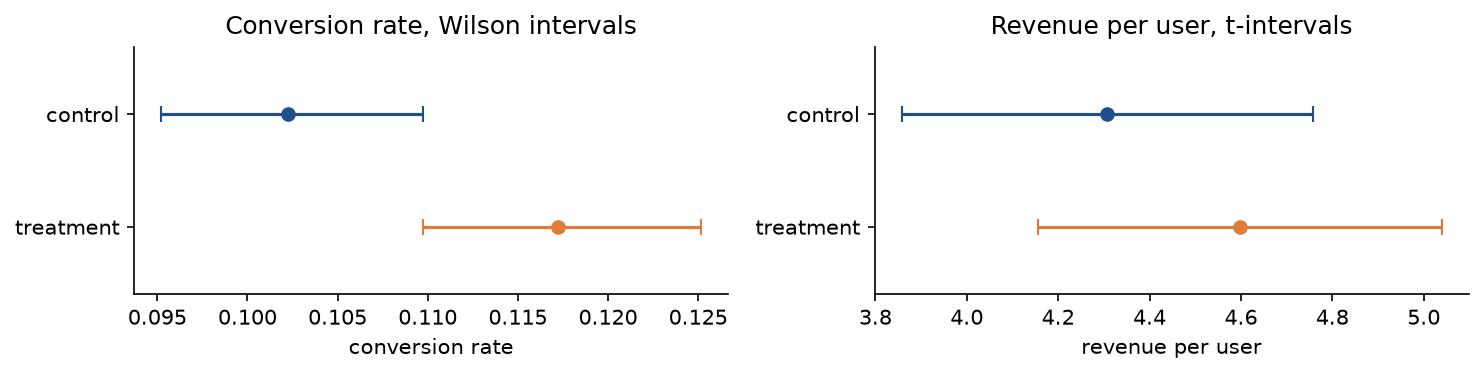
Left: the conversion rates of control and treatment with their Wilson intervals, the treatment interval starting where the control interval ends; right: the revenue per user of both groups with t-intervals that overlap widely

The two panels show the same users through two metrics. Overlapping or touching per-group intervals do not by themselves mean "no difference"; the interval for the difference, below, is the one to read.

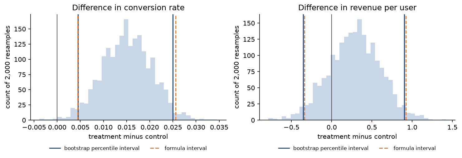
Bootstrap distributions of the difference in conversion rate and of the difference in revenue per user, each with the bootstrap percentile interval in blue and the formula interval dashed in orange: the conversion interval lies above zero, the revenue interval straddles it

The percentile interval and the formula interval nearly coincide for both metrics, which confirms the normal approximation behind the formulas at this sample size, even for the very skewed revenue.

The default seed, 4, gives a run whose estimated lift happens to equal the true one. Power 0.8 also means one run in five misses an effect of this size, and --seed 0 is such a run: the rates come out 0.1059 and 0.1088, z = 0.5466 and p = 0.5847. Options such as --baseline, --target, --power, --mean-order-value, --resamples, --aa-runs and --looks change the setup, and --figures sends the two PNGs to another folder so a custom run does not overwrite the ones shown here.

python foundations/probability-and-statistics/project/ab_test_report.py
python foundations/probability-and-statistics/project/ab_test_report.py --seed 0 --figures ab-test-figures

The notebook probability_and_statistics.ipynb is a guided tour in the order of this page: the dice and the screening test, the distributions and their samplers, correlation, the limit theorems, estimation, intervals, tests, the pitfalls, the iris data, a short A/B test and the comparison with SciPy. The tests in tests check the worked example value by value, the mathematical properties above, the simulations quoted here and the agreement with SciPy, and run in a few seconds:

python -m pytest foundations/probability-and-statistics

Data: everything except the iris analysis is synthetic, generated from fixed seeds. The iris analysis uses Fisher's iris measurements (R. A. Fisher, 1936), which scikit-learn ships with the library, so nothing is downloaded; the data set is distributed by the UCI Machine Learning Repository under the CC BY 4.0 licence.

In practice¶

Production code uses scipy.stats, and for every function here there is a SciPy or NumPy equivalent:

Distributions: Binomial(8, 0.25).pmf and Normal(10, 2).cdf correspond to scipy.stats.binom(8, 0.25).pmf and scipy.stats.norm(10, 2).cdf; note that SciPy writes the exponential with scale, the inverse of our rate.
Sampling distributions: student_t_cdf, chi_square_sf, f_sf and the quantile functions correspond to scipy.stats.t.cdf, chi2.sf, f.sf and the ppf methods.
Moments: sample_variance(x, ddof=1) and correlation correspond to np.var(x, ddof=1), np.corrcoef and scipy.stats.pearsonr.
Intervals: t_interval corresponds to scipy.stats.ttest_1samp(x, mu0).confidence_interval() or scipy.stats.t.interval, wilson_interval to scipy.stats.binomtest(k, n).proportion_ci(method="wilson"), and bootstrap_replicates with percentile_interval to scipy.stats.bootstrap(..., method="percentile").
Tests: one_sample_t_test, two_sample_t_test and paired_t_test correspond to scipy.stats.ttest_1samp, ttest_ind(equal_var=...) and ttest_rel; the chi-square tests to scipy.stats.chisquare and chi2_contingency(correction=False); one_way_anova to scipy.stats.f_oneway; and benjamini_hochberg to scipy.stats.false_discovery_control.

examples/compare_with_scipy.py evaluates every pair on grids of arguments and on the data of this page. The largest relative difference is 1.3 × 10⁻¹³, for the iris ANOVA p-value of 4.5 × 10⁻¹⁷; the distribution functions agree to within 6 × 10⁻¹⁴ everywhere, tails included, and the other test results to within 3 × 10⁻¹⁵. scipy.stats.bootstrap draws its resamples with rng.integers(0, n, (resamples, n)), as bootstrap_replicates does, so with the same seed the replicates are identical and so are the intervals. SciPy has no z-test; with a known σ it is two lines with scipy.stats.norm.sf. Holm's and Bonferroni's adjustments and the two-proportion sample size are not in SciPy and are checked against the worked examples and their defining properties only. The tests assert all of these agreements.

A realistic run on Fisher's iris data, sepal and petal length and width in centimetres for 50 flowers of each of three species, gives the same answers as SciPy:

The 95 % t-intervals for mean petal length are (1.4126, 1.5114) for setosa, (4.1265, 4.3935) for versicolor and (5.3952, 5.7088) for virginica, identical to scipy.stats.t.interval.
A one-way ANOVA of sepal width across the species gives F = 49.1600 on (2, 147) degrees of freedom with p = 4.492 × 10⁻¹⁷.
Welch's test of sepal length between versicolor and virginica gives t = -5.6292 on 94.0255 degrees of freedom with p = 1.866 × 10⁻⁷.
All twelve pairwise Welch tests, four measurements by three pairs of species, stay significant after Holm's and Benjamini-Hochberg's corrections; the weakest is sepal width between versicolor and virginica, with p = 0.0018.

The data also contain a textbook case of Simpson's paradox. Across all 150 flowers the correlation between sepal length and sepal width is -0.1176; within the species it is 0.7425, 0.5259 and 0.4572.

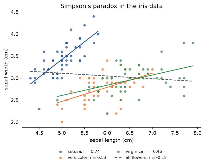
Sepal width against sepal length for the three iris species, each with its own rising regression line, and a dashed line for all flowers together that falls slightly

Setosa flowers have short, wide sepals and the other two species long, narrow ones, so pooling the species creates a downward trend that none of them shows. The species is a confounder of the pooled correlation.

When to use which:

Use the from-scratch functions to see what a test computes, to check a formula, or where a dependency on SciPy is unwelcome. Use scipy.stats for everything else: it covers far more distributions and tests, handles edge cases and vectorizes over axes.
For comparing two means, use Welch's test by default; scipy.stats.ttest_ind uses the pooled test unless equal_var=False. For paired measurements, use the paired test, which removes the variation between subjects.
For a proportion, report a Wilson interval rather than a Wald interval. For a statistic without a standard-error formula, use the bootstrap, preferably the BCa interval that scipy.stats.bootstrap computes by default.
For counts in a table, use the chi-square test when every expected count is at least about 5, and scipy.stats.fisher_exact or an exact permutation test otherwise.
For more than two groups, run one ANOVA and then corrected pairwise comparisons, for example Tukey's HSD (scipy.stats.tukey_hsd), instead of all pairwise t-tests.
With many tests, decide in advance what to control: the family-wise error rate (Holm) when a single false claim is costly, the false discovery rate (Benjamini-Hochberg) when screening many candidates.
For an A/B test, fix the sample size from a power calculation before the experiment, check the split, report the difference with its interval, and do not stop early unless the design was built for repeated looks.
statsmodels, which is not among this handbook's dependencies, adds z-tests, power calculations, two-way ANOVA and multipletests with Holm and many other procedures.

Pitfalls¶

Confusing P(A | B) with P(B | A). A test that is positive for 96 % of people with the condition does not mean that 96 % of positive people have it: at a prevalence of 1.5 % only 19.59 % do. Always ask for the base rate; the base-rate figure shows the same test at every prevalence.
Reading a p-value as the probability that the null hypothesis is true. The p-value is the probability of data this extreme given H0, not the probability of H0 given the data. A significance test is a screening test for hypotheses, with power as its sensitivity and 1 - α as its specificity: if one tested hypothesis in ten is true and power is 0.5, then 0.4737 of the results with p < 0.05 are false, and 0.9083 if one in a hundred is true (false_discovery_share, printed by examples/testing_pitfalls.py).
Reading "not significant" as "no effect", or "significant" as "important". The thermometer's p = 0.1405 comes with an estimated bias of 0.6 °C and an interval reaching 1.51 °C: absence of evidence, not evidence of absence. The project's revenue difference, p = 0.3664, is likewise undecided rather than zero. Conversely, with a large enough sample a negligible effect becomes significant. Report the estimate and its interval, not only the p-value.
Misreading a confidence interval. "There is a 95 % probability that μ lies in (3.6918, 5.5082)" is wrong in the frequentist framework: the 95 % is the long-run coverage of the procedure, 0.9516 in the simulation. A statement about the probability of μ needs a prior and a posterior, as in the MAP example.
Using the normal critical value with an estimated standard deviation. For n = 5, 1.96 instead of 2.7764 turns the thermometer's p = 0.1405 into 0.0666 and lowers the coverage of a nominal 95 % interval to 0.8778. The t quantile is 4.3027 with 2 degrees of freedom, 2.2622 with 9, still 2.0452 with 29 and 1.9842 with 99.
Confusing the standard deviation with the standard error. s = 0.7314 describes the spread of single readings and s/√n = 0.3271 the uncertainty of their mean; an interval for the mean built from s is √5 times too wide, and a check of single readings against s/√n flags far too many as outliers.
Dividing by n or by n - 1 without noticing. np.var and np.std divide by n unless given ddof=1, pandas divides by n - 1, and the standard library has pvariance and variance; for the thermometer that is 0.428 against 0.535 (variance_conventions). Remember also that s is biased for σ even though s² is unbiased for σ².
Treating "mutually exclusive" as "independent". Disjoint events with positive probabilities are always dependent; independence means the joint probability factorizes, as for "first die even" and "sum 7".
Treating a density as a probability. The density of Uniform(0, 0.5) is 2 and that of Normal(0, 0.1²) at its mean is 3.9894; only areas under a density are probabilities.
Reading correlation as causation, or zero correlation as independence. A common cause produces a correlation of 0.7353 between variables that do not influence each other (0.7342 in 20,000 simulated draws), which vanishes under intervention (-0.0095); Y = X² has zero correlation with X (0.0064 simulated) although it is completely determined by it; and in the iris data the pooled correlation of -0.1176 reverses to positive within every species. The correlation figure and the Simpson figure show all three.
Expecting every average to settle down. The law of large numbers and the central limit theorem need a finite mean and a finite variance. Heavy-tailed data, such as Cauchy draws, give averages that jump around forever; the median is the robust alternative.
Peeking at the data and stopping when p < 0.05. Testing after every batch of 10 values, up to 10 batches, raises the false positive rate from 0.05 to 0.1936, and with 50 looks to 0.3175, while testing once at the end stays near 0.05 (peeking_table). The A/A check of the sample project shows the same inflation, 0.1950 with 10 looks. Fix the sample size in advance or use a sequential method designed for repeated looks.
Running many tests without correction. Twenty tests of true nulls produce at least one false positive with probability 0.6415. Testing all ten pairs of five identical groups finds a "difference" in 0.2873 of experiments, against 0.0500 for one ANOVA (pairwise_versus_anova).
Pooling variances that differ. With 10 values of standard deviation 3 against 40 of standard deviation 1, Student's pooled test rejects a true null in 0.2525 of the cases at α = 0.05 and Welch's test in 0.0489 (pooled_variance_false_positives). Welch costs almost nothing when the variances are equal, so use it by default.
Computing chi-square from percentages, or with small expected counts. The statistic scales with the number of observations: the failure table gives 4.704 from counts, 47.04 with ten times the data and 1.568 from percentages of the total. Use counts, and switch to an exact test when expected counts fall below about 5. Note also that scipy.stats.chi2_contingency applies Yates' continuity correction to 2 by 2 tables by default, 0.6992 instead of 1.0362 for the first two rows of the failure table.
Using the Wald interval for a proportion. Its exact coverage at p = 0.02 and n = 40 is 0.5531 for a nominal 0.95, and for zero successes it has width zero. Use the Wilson interval.
Trusting a maximum likelihood estimate from zero counts. 0 passes in 4 runs gives an estimate of 0, a claim of impossibility. A Beta prior, which amounts to add-one smoothing for the uniform prior, gives 0.1667; naive Bayes needs the same correction for words never seen with a class.
Mis-stated ANOVA facts. Some summaries describe two-way ANOVA as a comparison of two groups. Two-way ANOVA has two categorical factors, for example cache setting and server type, and can test their interaction; two groups are compared by a t-test, which a one-way ANOVA with two groups reproduces with F = t². The degrees of freedom of the F ratio are k - 1 and N - k, not N - 1 or n - 1 per group. And a significant F only says that not all means are equal; which ones differ needs a post-hoc procedure.
Analysing an A/B test whose split is broken. If users are not placed in the groups by a fair, independent mechanism, a difference between the groups may come from who landed where rather than from the treatment. Check the split against 50 / 50 with a goodness-of-fit test before reading any other number, as the sample project does.