Ensembles

A single decision tree is easy to grow and easy to read, but it is unstable: change a few training rows and the tree, and its predictions, change a lot. A single decision stump is stable but far too simple. Ensembles fix both problems by combining many models. Bagging and random forests average many deep trees grown on perturbed copies of the data, which cancels much of their variance; boosting fits simple models one after another, each concentrating on what the previous ones got wrong, which removes bias. This page derives why averaging helps and where it stops helping, works out bootstrap sampling and the out-of-bag error, measures how random forests decorrelate their trees, runs AdaBoost round by round on ten points with every weight shown, by reweighting and by resampling, derives AdaBoost as stagewise minimization of the exponential loss, builds gradient boosting from residual fitting and extends it to classification with Newton steps, and checks everything against scikit-learn on a real medical data set. Afterwards you will be able to compute a boosting round by hand, explain why a forest's error stops falling as trees are added, choose between the methods and spot the common mistakes in implementations and in their evaluation. It builds on Decision trees.

To run the code in this topic, install the base and ml groups.

Intuition

Ask many people to guess the weight of an ox and average the answers: the average is usually closer than most individual guesses, because the errors partly cancel. They cancel only to the extent that they are independent. If everyone copied the loudest guesser, averaging would change nothing. Ensembles of models face the same trade. Models trained on the same data make similar mistakes, and the similarity, not the number of models, decides how much averaging can achieve.

Two families follow from two ways of making models differ.

• Averaging methods train flexible models, typically fully grown decision trees, each on a bootstrap sample (rows drawn with replacement), and average their predictions. Each tree has low bias and high variance; the average keeps the low bias and loses much of the variance. That is bagging. A random forest adds a second source of randomness, a random subset of candidate features at every split, so that the trees resemble each other less and their average cancels more.
• Boosting trains weak models, such as one-split stumps, one after another. Each round raises the weight of the rows the ensemble still gets wrong, so the next model is forced to work on them, and the final prediction is a weighted vote in which better models count more. A stump on its own has high bias; a weighted sum of hundreds of stumps can draw a complicated boundary.

In the averaging family the trees never see each other: they can be grown in parallel, and the only link between them is the data they share. In the boosting family every learner depends on all the ones before it, through the weights it is trained on, so the rounds run in sequence. A third idea, stacking, learns how to combine the models instead of fixing the rule in advance; it is described near the end of the next section.

How it works

Notation

The training set has n rows, each with p features, and a label or target. An averaging ensemble has B models, and the prediction of model b at an input is written with a hat. A boosting run has T rounds; in round t the weak learner is h, the weight of row i is w, the weighted error is ε, and β and α are derived from ε. In boosting the labels are coded as -1 and +1. The formula images write the round as a subscript t, or as a superscript (t) on the weights; the text writes them plainly, for example "the weight w of row i in round t" or ε1 for the error of round 1. Square brackets around a statement in a formula mean 1 if the statement is true and 0 if it is not.

Why averaging reduces variance

Fix an input and treat the B predictions there as random variables, random because the training data and the bootstrap draws are. Suppose they share a mean, a variance σ² and a pairwise correlation ρ, so that the covariance of two different predictions is ρσ². The mean of their average is the shared mean: averaging leaves the bias unchanged. Its variance is a double sum of covariances with B terms on the diagonal and B(B - 1) off it:

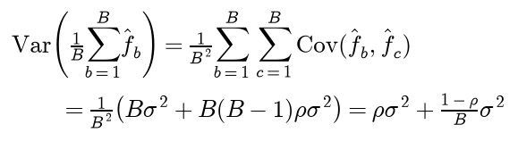
The second term disappears as B grows; the first does not. With σ² = 4 and ρ = 0.3, ten models give 1.2 + 0.28 = 1.48, and no number of models gets below ρσ² = 1.2. Adding trees to a forest therefore never hurts its accuracy, but the gains flatten out at a level set by ρ, and the only way below it is to make the models less correlated without making each one much worse. That is the design brief of the random forest.

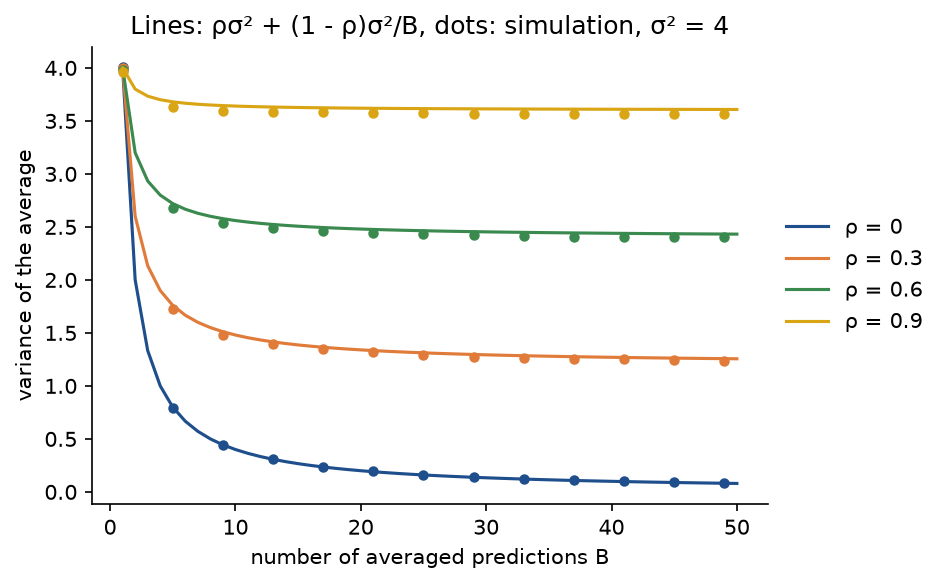
The lines are the formula and the dots a simulation of correlated predictions. Uncorrelated predictions keep falling towards zero; with ρ = 0.9, averaging fifty predictions removes only a tenth of the variance.

For classifiers the same effect appears in the vote. If B classifiers (an odd number) are each right with probability q above one half and err independently, the majority is right when more than half of them are:

For q = 0.6 this is 0.6826 with five voters, 0.8462 with 25 and 0.9791 with 101. Real classifiers trained on one data set are far from independent, so the gain is much smaller, and if q is below one half the vote makes things worse.

Bootstrap samples and the out-of-bag error

A bootstrap sample draws n rows from the n training rows, uniformly and with replacement. One draw misses a given row with probability 1 - 1/n, and the n independent draws all miss it with that probability raised to the power n, so

For n = 10 the probability is 1 - 0.9 to the power 10 = 0.6513, so a sample contains 6.5132 distinct rows on average; by n = 1000 it is 0.6323. Every bootstrap sample has the full size n and repeats about a third of its rows. Unlike a mini-batch, which draws without replacement, the same row can appear several times.

Bagging (bootstrap aggregating) draws B bootstrap samples, fits one model to each and combines them: the average for regression, a vote for classification. The rows a sample did not draw, about 36.8 % of them, are that model's out-of-bag rows. The out-of-bag prediction for row i combines only the models that did not see row i:

The out-of-bag error is the error of these predictions over all rows. Each prediction comes from models that never saw the row, so it estimates the test error without setting rows aside.

The estimate comes free with the forest, but it describes an ensemble of about 0.368B trees, not B, and is therefore slightly pessimistic, noticeably so when B is small. With few trees some rows are out of bag for none of them: a row is in all B samples with probability about 0.632 to the power B, which is still 1 % for B = 10.

Random forests

A random forest is bagging of trees with one change: at every split, the tree may choose only among m features drawn at random from the p, fresh for each split. Breiman's defaults are m equal to the square root of p, rounded down, for classification and p/3 for regression; scikit-learn uses the square root of p for classification and all p features for regression. With m = p the forest is bagging.

The effect is on ρ. Without the restriction, every tree splits first on the same strong features and the trees look alike. With small m, the strong features are often unavailable and the trees diverge, so ρ falls. The price is a weaker individual tree: higher σ² and often higher bias, because some splits are forced onto poor features. Whether the trade pays off depends on the problem, and it can be measured. The Friedman regression problem has ten features uniform on [0, 1], a target that uses only the first five, and unit Gaussian noise:

examples/forest_experiments.py draws 20 independent training sets of 200 rows, grows a 25-tree regression forest with leaves of at least five rows on each, and predicts 200 fixed test points. For each test point the variance of a single tree splits into a part due to the training set, the variance of the forest mean across training sets corrected for the finite forest, and a part due to the bootstrap and feature draws, the variance within a forest. Averaging both parts over the test points gives the correlation:

The results, with errors measured as mean squared differences from the noise-free target, listed as ρ, the variance of one tree, the forest variance, the squared bias, the forest error and the error of one tree:

• m = 1: 0.034, 11.923, 0.870, 12.021, 12.847 and 23.900.
• m = 2: 0.043, 11.808, 0.956, 8.010, 8.917 and 19.770.
• m = 3: 0.055, 11.031, 1.020, 6.363, 7.332 and 17.344.
• m = 5: 0.082, 9.424, 1.122, 5.118, 6.184 and 14.486.
• m = 7: 0.114, 8.419, 1.260, 4.723, 5.920 and 13.079.
• m = 10: 0.159, 7.700, 1.481, 4.420, 5.828 and 12.047.

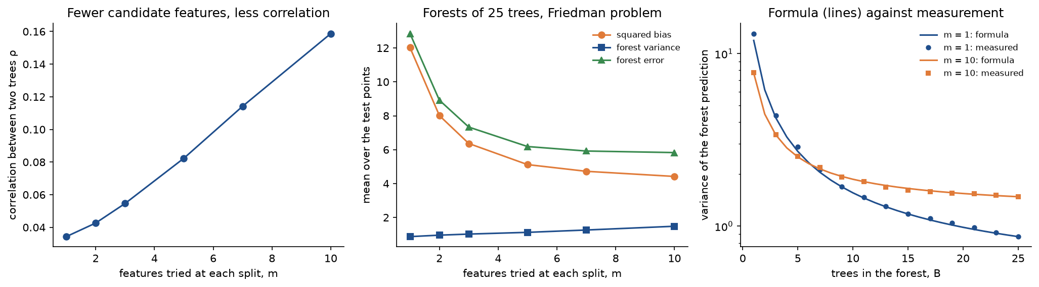
Feature subsampling does what it promises: the correlation between trees falls from 0.159 with all ten features to 0.034 with one, and the forest variance falls from 1.481 to 0.870. But half the features are noise, a tree that may only look at one random feature per split often has to split on noise, and the squared bias rises from 4.420 to 12.021. Here the bias wins and bagging (m = 10) is best, which is why scikit-learn's regression forests use every feature by default. On the breast cancer data used by the project, where nearly every feature carries signal, a small m costs little bias: out-of-bag accuracies of 200-tree forests on all 569 rows are 0.9631 for m = 1, 0.9596 for 2, 0.9631 for 5, 0.9684 for 10, 0.9666 for 20 and 0.9561 for m = 30, which is bagging. The right panel checks the variance formula on real trees: ρ and σ² are estimated once from the 25-tree forests, and the formula follows the measured variance of forests made of their first B trees.

Hard and soft voting

For a classifier with K classes, hard (majority) voting predicts the class most models predict; soft voting averages the predicted class probabilities and takes the largest:

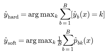
Three models that give class 1 the probabilities 0.90, 0.40 and 0.45 vote 1, 0, 0, so the majority says 0, while the mean probability is 0.5833 and soft voting says 1. Soft voting uses how confident each model is, which helps when the probabilities mean something. scikit-learn's forests and BaggingClassifier vote softly. A fully grown tree has pure leaves and predicts probabilities of exactly 0 or 1, and then the two rules agree.

AdaBoost

AdaBoost.M1 keeps one weight per training row, starting at 1/n for every row. In round t = 1, ..., T it fits the weak learner to the weighted rows, measures its weighted error, stops if the error is not below one half, and otherwise computes β and the vote weight α and updates the weights:

The final classifier is the sign of the weighted vote, ties going to the first class:

A decision stump makes a good weak learner: one threshold on one feature, with each side predicting its weighted majority, chosen to minimize the weighted error.

Normalization keeps the weights a probability distribution. It is needed for ε to be an error rate between 0 and 1, comparable with one half, and it gives AdaBoost its defining property. After the multiplication the misclassified rows still weigh ε in total and the correct ones (1 - ε)β = ε, so after dividing by 2ε each group weighs exactly one half:

The learner just used has error exactly one half on the new distribution, a coin flip, so the next round must find something it does not already know.

Several equivalent forms of the update circulate. Multiplying the misclassified rows by 1/β = e to the power α instead of the correct ones by β gives the same weights after normalization, and so does the symmetric form in the first line below; some texts call α/2 the vote weight. Scaling every vote weight by the same constant, including changing the base of the logarithm, leaves the classifier unchanged. For K > 2 classes AdaBoost.M1 still needs ε below one half, which is hard for a stump; SAMME, the variant in scikit-learn, adds ln(K - 1) to the vote weight and only needs ε below 1 - 1/K. For two classes the two coincide.

When the weak learner cannot take weights, boosting by resampling draws a sample of n rows with replacement and probabilities equal to the weights, fits the learner to the sample without weights, and computes ε as above, on all n rows with their weights, not on the sample. If ε is not below one half, it draws again. The rest of the round is unchanged: every row is updated according to whether it is classified correctly, whether or not it was drawn, and the normalization runs over all n rows.

AdaBoost as forward stagewise additive modelling

Consider additive models, weighted sums F of weak learners, and the exponential loss e to the power -yF, which is small when the margin yF is large and positive. Forward stagewise fitting adds one term at a time and never revisits earlier ones. With the score F of the earlier rounds fixed, adding c times a learner h gives

Since y times h(x) is +1 for a correct row and -1 for a wrong one, the sum splits into

For any c > 0 the best h is the one with the smallest weighted error under the weights v. With ε that error after normalizing the v, setting the derivative with respect to c to zero gives

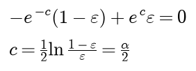
The new weights are v times e to the power -cyh, which multiplies the wrong rows by e to the power 2c = (1 - ε)/ε relative to the correct ones, exactly AdaBoost's update. So AdaBoost.M1 is forward stagewise minimization of the exponential loss with F equal to half the weighted vote, and its weights in round t are the normalized loss terms of the earlier rounds' score. Two consequences:

• The normalizer of the symmetric update is the factor by which the average exponential loss falls in round t. Because a mistake has a margin of at most zero and so a loss term of at least 1, the training error is bounded by the average exponential loss, and after T rounds by a product that shrinks geometrically as long as every ε stays below one half by a margin:

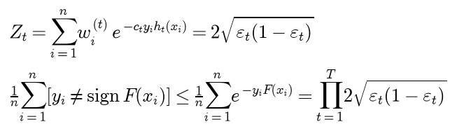
The bound is loose, but it explains why AdaBoost's training error keeps falling.

• The minimizer of the expected exponential loss is half the log-odds, the same target as logistic regression:

The exponential loss punishes a confidently wrong prediction far more than the logistic loss does, which is why AdaBoost reacts badly to mislabelled rows.

Gradient boosting

Forward stagewise fitting works for any differentiable loss if each step moves F a little in the direction that lowers the loss fastest, evaluated at the training points: the negative gradient of the loss with respect to the score. A regression tree fitted to these values generalizes the step to new inputs. For squared error the negative gradient is the residual, and the algorithm becomes residual fitting:

Each leaf of the tree predicts the mean residual of its rows, the best constant for squared error. The learning rate ν, between 0 and 1, shrinks every step. With ν = 1 each tree removes as much of the residual as it can and the training error falls fastest, but the model soon fits noise; a small ν needs proportionally more trees and usually reaches a lower test error. The number of trees is then the main thing to tune, by early stopping on held-out rows: training error falls for ever.

For a binary label coded 0 and 1 the same loop runs on the logistic loss (log loss). The score F is now the log-odds of class 1, the start is the log-odds of the share of class 1, and the negative gradient is y - p with p the sigmoid of the score. A tree is fitted to y - p by squared error as before, but its leaf values are then replaced by one Newton step on the loss of the rows in the leaf, which accounts for the curvature p(1 - p):

This is what scikit-learn's GradientBoostingClassifier does, and the comparison under In practice shows that the two agree stage by stage.

XGBoost and its successors make the Newton view the whole algorithm. They expand the loss to second order around the current scores, with g and h the first and second derivatives of the loss of each row:

For a leaf j containing the rows I, with G and H the sums of g and h over those rows, a penalty λ on large leaf values and a cost γ for each extra leaf, the objective is minimized by a Newton step, and a split is worth its gain:

For squared error, with λ = 0, the leaf value is the mean residual and the gain is half the drop in squared error, exactly the residual-fitting tree above. For the log loss the curvature matters, and with λ = 0 the leaf value is the Newton step of scikit-learn's classifier.

Shrinkage is easy to see on the Friedman problem. examples/gradient_boosting_by_hand.py fits depth-3 trees to 500 rows and scores them on 2,000 fresh rows, whose noise variance is 1:

• ν = 1: best test error 5.2571 after 5 trees; after 1,500 trees the test error is 6.2446 and the training error 0.0000.
• ν = 0.3: best 2.7768 after 90 trees; after 1,500 trees 2.8172, training error 0.0000.
• ν = 0.1: best 2.4284 after 353 trees; after 1,500 trees 2.4526, training error 0.0001.
• ν = 0.03: best 2.4064 after 1,267 trees; after 1,500 trees 2.4125, training error 0.0500.

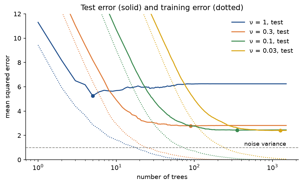
Without shrinkage the model is at its best after five trees and then fits the noise; with ν = 0.1 or less it needs hundreds of trees, but its best test error is less than half as large. The training error reaches zero in every run and says nothing about when to stop.

Stacking

Stacking fits a second-level model, the meta-learner, to the predictions of several first-level models. The meta-learner must be trained on predictions the first-level models made for rows they did not see, usually out-of-fold predictions from k-fold cross-validation; otherwise it learns how well each model fits its own training rows, which says little about new rows. After that the first-level models are refitted on all training rows, and their predictions for new rows go through the meta-learner. A regularized logistic regression is the usual meta-learner.

Stacking works best with first-level models that are good and different, so that their mistakes fall on different rows; three forests with different seeds would add little.

Feature importance

The impurity importance (mean decrease in impurity) of feature j in one tree adds up the weighted drop in impurity over every node s that splits on j, where W is the training weight in a node and i its Gini impurity or variance; a forest averages its trees, and the result is normalized to sum to one:

It is free, but it is measured on the training rows, so splits that only fit noise count too, and features with many possible thresholds collect more of them. Permutation importance instead shuffles the values of one feature in held-out data, which breaks its link to the target while keeping its distribution, and records the drop in the score:

It measures what the fitted model actually relies on, at the cost of extra predictions, and it underrates features whose information is duplicated by others. On the breast cancer data used by the project, with two noise columns appended, a standard normal one and a fair coin, the impurity importances of a 200-tree forest put worst area, worst concave points and mean concave points on top and rank the noise columns 27th and 32nd of 32, with importances 0.0035 and 0.0004. Permutation importance on the test rows gives both noise columns exactly zero, but no real feature more than 0.0080 either.

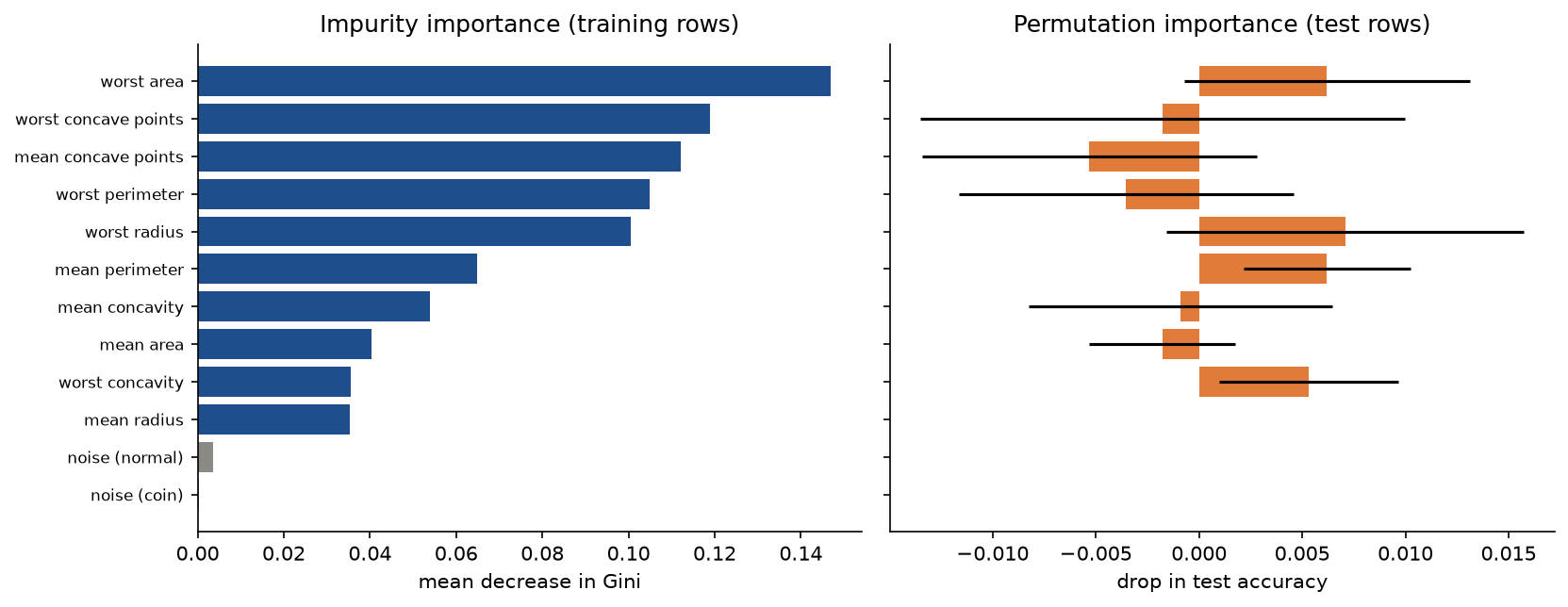
The 30 features come in near-duplicate groups (radius, perimeter and area, for example), and when one is shuffled the trees use its siblings, so permutation importance cannot single any of them out. examples/common_mistakes.py draws this figure.

Worked example

AdaBoost by reweighting

Ten points with two integer features x1 and x2, and labels -1 and +1:

• Label +1: row 2 at (1, 6), row 4 at (9, 9), row 5 at (10, 5) and row 10 at (4, 4).
• Label -1: row 1 at (3, 3), row 3 at (6, 7), row 6 at (2, 10), row 7 at (5, 1), row 8 at (7, 2) and row 9 at (8, 8).

The weak learner is a stump that thresholds one feature halfway between two neighbouring values and lets each side predict its weighted majority; the stump with the smallest weighted error wins. Weights are shown to four decimals, with exact fractions where they are short.

Round 1. All weights are 0.1. The best stump on each feature:

• On x1: x1 ≤ 8.5 predicts -1, otherwise +1. It gets rows 2 and 10 wrong, weighted error 0.2.
• On x2: x2 ≤ 3.5 predicts -1, otherwise +1. It gets rows 3, 6 and 9 wrong, weighted error 0.3.

The first stump wins: rows 4 and 5 are the only points with x1 above 8.5 and both are +1, and the two +1 points on the left, rows 2 and 10, are its mistakes. So ε1 = 0.2, β1 = 0.2/0.8 = 0.25 and α1 = ln 4 = 1.3863. The eight correct rows drop to 0.1 × 0.25 = 0.025; rows 2 and 10 stay at 0.1. The total is 8 × 0.025 + 2 × 0.1 = 0.4 = 2ε1, and dividing by it gives 1/16 = 0.0625 for the eight correct rows and 1/4 = 0.25 for rows 2 and 10. The two mistakes now carry half the weight between them.

Round 2. Under the new weights:

• On x1: x1 ≤ 4.5 predicts +1, otherwise -1. It gets rows 1, 4, 5 and 6 wrong, weighted error 4 × 0.0625 = 0.25.
• On x2: x2 ≤ 3.5 predicts -1, otherwise +1. It gets rows 3, 6 and 9 wrong, weighted error 3 × 0.0625 = 0.1875.

The stump that lost round 1 with an error of 0.3 wins round 2: it classifies rows 2 and 10 correctly, and they now weigh four times as much as any other row. ε2 = 3/16 = 0.1875, β2 = 3/13 = 0.2308 and α2 = ln(13/3) = 1.4663. Multiplying the seven correct rows by 3/13 turns 1/16 into 3/208 = 0.0144 and 1/4 into 3/52 = 0.0577; rows 3, 6 and 9 keep 0.0625. The total is 0.375 = 2ε2, and after normalization the weights are:

• 1/26 = 0.0385 for rows 1, 4, 5, 7 and 8,
• 2/13 = 0.1538 for rows 2 and 10,
• 1/6 = 0.1667 for rows 3, 6 and 9, the round's mistakes, which again weigh 3 × 1/6 = 1/2 together.

Round 3. Under these weights:

• On x1: x1 ≤ 1.5 predicts +1, otherwise -1. It gets rows 4, 5 and 10 wrong, weighted error 1/26 + 1/26 + 2/13 = 0.2308.
• On x2: x2 ≤ 6.5 predicts +1, otherwise -1. It gets rows 1, 4, 7 and 8 wrong, weighted error 4 × 1/26 = 0.1538.

The x1 stump puts only row 2 on the +1 side and so misses the other three +1 rows, one of them heavy. The x2 stump gets the heavy rows 3, 6 and 9 right and pays only for four light rows: ε3 = 2/13 = 0.1538, β3 = 2/11 = 0.1818 and α3 = ln 5.5 = 1.7047. After the update the four mistakes weigh 1/8 = 0.125 each, and the correct rows are rescaled by 13/22 to 1/11 = 0.0909 for rows 2 and 10, 13/132 = 0.0985 for rows 3, 6 and 9 and 1/44 = 0.0227 for row 5.

The vote. The three stumps alone are right on 8, 7 and 6 of the ten rows. The weighted vote 1.3863 h1 + 1.4663 h2 + 1.7047 h3 gets all ten:

• Rows 1, 7 and 8: the stumps say -1, -1, +1, score -1.1479, label -1.
• Rows 2 and 10: -1, +1, +1, score 1.7848, label +1.
• Rows 3, 6 and 9: -1, +1, -1, score -1.6247, label -1.
• Row 4: +1, +1, -1, score 1.1479, label +1.
• Row 5: +1, +1, +1, score 4.5574, label +1.

Adding the rounded vote weights gives 1.7847 for rows 2 and 10 and 4.5573 for row 5; the list shows the full-precision values.

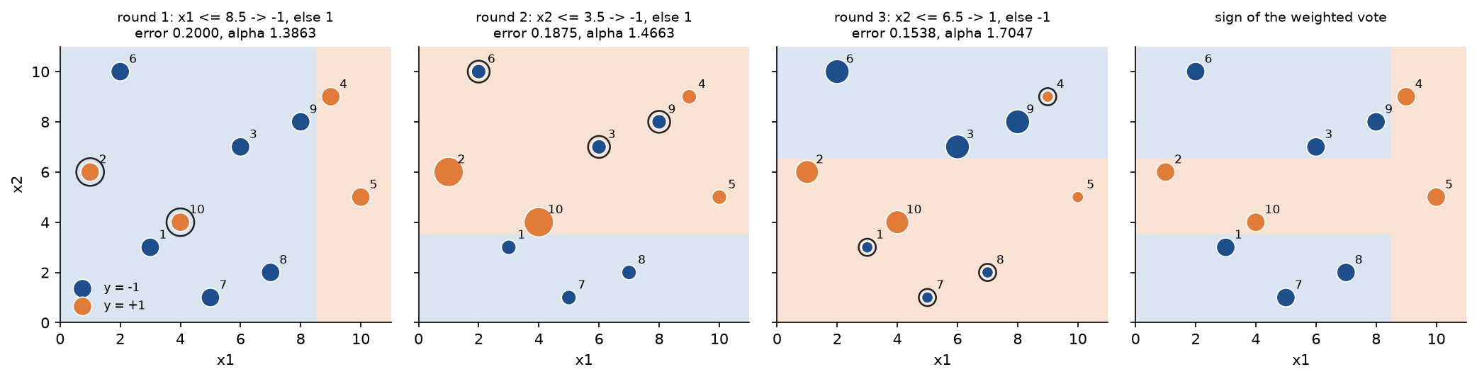
The growing and shrinking markers show the reweighting at work: the ringed mistakes of one round are the large markers of the next. No single stump separates the two classes, but the vote of three draws a staircase that does.

The exponential-loss view

The training-error bound after the three rounds is the product of 2√(0.2 × 0.8), 2√(0.1875 × 0.8125) and 2√((2/13)(11/13)), with partial products 0.8, 0.6245 and 0.4506; the actual training error is 0. The average exponential loss of half the final vote is exactly 0.4506, the bound. A grid search for the step along h3 that minimizes the exponential loss, starting from half the vote of the first two rounds, finds 0.852, and α3/2 = 0.8524.

Boosting by resampling, with the correct and a broken normalization

Boosting by resampling with seed 5 draws rows 1, 1, 1, 3, 4, 5, 6, 9, 9, 10 in round 1. Rows 2, 7 and 8 are not drawn. The best stump on the sample is again x1 ≤ 8.5. Its error is measured on all ten rows with their weights: rows 2 and 10 are wrong, so ε1 = 0.2, although row 2 never appeared in the sample. On the sample alone the error would be 1/10, and the vote weight ln 9 = 2.1972 instead of ln 4. With every row updated and the normalization over all ten rows, the weights after round 1 are exactly those of reweighting, 1/16 and 1/4. The second sample, rows 1, 2, 4, 4, 5, 8, 8, 10, 10, 10, again gives x2 ≤ 3.5 and the same weights as round 2 above.

A variant that appears in some write-ups updates and rescales only the rows that were drawn. It multiplies the correctly classified drawn rows by β1 and then rescales the drawn rows so that their sum over the sample, duplicates counted, is what it was before; the rows that were not drawn keep their weights. In round 1 every row starts at 0.1, and:

• Rows 1, 3, 4, 5, 6 and 9, drawn and right, drop to 0.025 and are rescaled to 0.0769.
• Row 10, drawn and wrong, keeps 0.1 and is rescaled to 0.3077.
• Row 2, not drawn and wrong, keeps 0.1.
• Rows 7 and 8, not drawn and right, keep 0.1.

The sum over the sample is 3 × 0.1 + 6 × 0.1 + 0.1 = 1 before and 3 × 0.025 + 4 × 0.025 + 2 × 0.025 + 0.1 = 0.325 after the multiplication (row 1 three times, rows 3, 4, 5 and 6 once, row 9 twice and row 10 once), hence the factor 1/0.325 = 3.0769. Three things have gone wrong:

• The weights add up to 6 × 0.0769 + 0.3077 + 3 × 0.1 = 1.0692, not 1.
• The update depends on whether a row was drawn. Row 2 is a mistake but keeps 0.1, while row 10, the same kind of mistake, rises to 0.3077; rows 7 and 8 are correct but are not down-weighted. The correct values are 0.25 for both mistakes and 0.0625 for every correct row.
• The stump just used has weighted error (0.1 + 0.3077)/1.0692 = 0.3813 under the new weights instead of exactly one half, so the next round is not pushed towards new information.

In round 2 the variant draws rows 1, 3, 6, 6, 7, 9, 9, 10, 10, 10 and picks x2 ≤ 5.5 for +1, otherwise -1, which is wrong on rows 1, 2, 4, 7 and 8. Its error, the sum of the weights of those rows, is 0.4538, a sum over weights that total 1.0692; as a fraction of the total it is 0.4245. The vote weight ln(0.5462/0.4538) = 0.1851 is tiny and the total after round 2 is 1.0874. On a real data set the drift continues until the inflated errors pass one half and boosting stops; see Pitfalls.

Gradient boosting by hand

Six points x = 1, ..., 6 with targets y = (5, 3, 2, 4, 7, 9), regression stumps and learning rate ν = 0.5. At every stage:

• F0 = 30/6 = 5 everywhere, mean squared error 5.6667. The residuals are (0, -2, -3, -1, 2, 4).
• The best stump on those residuals splits at x ≤ 4.5. The left mean is (0 - 2 - 3 - 1)/4 = -1.5 and the right mean (2 + 4)/2 = 3, which lowers the sum of squared residuals from 34 by (4 × 2 / 6) × (3 - (-1.5))² = 27, more than any other split.
• Half a step gives F1 = (4.25, 4.25, 4.25, 4.25, 6.5, 6.5), mean squared error 2.2917. The residuals are (0.75, -1.25, -2.25, -0.25, 0.5, 2.5).
• The best split is now x ≤ 5.5, with means (0.75 - 1.25 - 2.25 - 0.25 + 0.5)/5 = -0.5 and 2.5.
• Half a step gives F2 = (4, 4, 4, 4, 6.25, 7.75), mean squared error 1.3542, with residuals (1, -1, -2, 0, 0.75, 1.25).

The second stump separates the point at x = 6, which the first step left furthest from its target. With the second-order formulas, g = F0 - y and h = 1: the right leaf of the first stump has G = -6 and H = 2, so the Newton step is 3 with λ = 0, the mean residual, and 6/3 = 2 with λ = 1. The gain of the split x ≤ 4.5 with λ = γ = 0 is 13.5, half of the drop of 27 in the sum of squared residuals. For the log loss at score 0, four rows with labels 1, 1, 0 and 1 have g = (-0.5, -0.5, 0.5, -0.5) and h = 0.25 each, and the Newton step of a leaf holding them is 1/1 = 1.

Every number in this section is asserted by tests/test_adaboost.py, tests/test_exponential_loss.py, tests/test_gradient_boosting.py, tests/test_second_order.py and tests/test_trace.py, and printed by examples/adaboost_by_hand.py and examples/gradient_boosting_by_hand.py.

The code

The package ensembles is plain NumPy, split into one module per idea. scikit-learn is imported only inside load_breast_cancer_data and the functions of comparisons.py, so everything else works without it.

• arrays.py holds the array types and as_features, which insists on one example per row.
• averaging.py holds the variance of an average, simulated correlated predictions, the majority-vote accuracy, the measurement of ρ and σ² from real trees, and the hard and soft voting rules.
• bootstrap.py holds the inclusion probability, bootstrap draws and out-of-bag rows.
• splits.py holds the split search: per-node statistics, impurities, leaf values and best_split, which scores every threshold of every candidate feature at once.
• tree.py holds the frozen Tree, stored as flat arrays like scikit-learn's trees, with apply, predict, predict_proba and feature_importances.
• growing.py holds fit_tree, a CART-style tree with weighted Gini impurity, weighted misclassification error or squared error, depth and leaf-size limits and random feature subsets per split.
• forest.py holds fit_forest, with fit_bagging and fit_random_forest as shortcuts, and the Forest with soft or hard voting, staged predictions, out-of-bag values and scores and impurity importances; feature_sampling="tree" gives the random subspace method instead.
• adaboost.py holds fit_adaboost by reweighting or resampling, with normalization="all" (correct) or "sampled" (the broken variant), and an AdaBoost that keeps every round's weights, sample, stump, error, β and α.
• exponential_loss.py holds the exponential loss, the stagewise coefficient and the training-error bound.
• gradient_boosting.py holds fit_gradient_boosting for squared error and for the log loss, with Newton leaves for the latter.
• second_order.py holds the derivatives of both losses, the Newton leaf value and the gain of a split.
• stacking.py holds out-of-fold predictions, a small nearest-neighbour model and a logistic meta-learner fitted by Newton's method.
• evaluation.py holds accuracy, mean squared error, stratified splits and folds, cross-validation and permutation importance.
• datasets.py holds the two worked examples, the Friedman problem, a synthetic classification problem, the data for the importance pitfall and the breast cancer loader.
• trace.py prints the worked examples round by round; pitfalls.py holds the quantities only a mistaken implementation computes.
• experiments.py runs the measurements behind the plots; benchmark.py holds the project's comparison; plotting.py, averaging_figures.py and boosting_figures.py draw every figure in the handbook's four colours.
• comparisons.py builds the same models in scikit-learn on the same samples and settings.

The split search of fit_tree sorts each candidate column, accumulates the weighted class counts, or the weighted sums of the target, down the sorted rows and scores every threshold at once. For Gini it maximizes the score below, where c is the weight of class k on a side and W the side's total weight; it orders splits exactly as the impurity decrease does, because the parent's impurity is the same for every candidate:

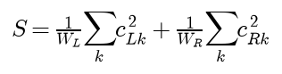
Thresholds lie halfway between neighbouring distinct values; ties go to the lowest feature index and then the lowest threshold. A round with zero error ends the AdaBoost loop and keeps its stump with vote weight 1, the convention scikit-learn uses. Bagging passes the bootstrap counts to the tree as row weights, which grows the same tree as duplicating the rows and is what scikit-learn does. The AdaBoost update is short enough to show whole:

if normalization == "all":
    updated = np.where(misclassified, weights, weights * beta)
    return updated, updated * (weights.sum() / updated.sum())
multiplicity = np.bincount(sample, minlength=weights.size).astype(np.float64)
drawn = multiplicity > 0
updated = np.where(drawn & ~misclassified, weights * beta, weights)
factor = np.sum(multiplicity * weights) / np.sum(multiplicity * updated)
return updated, np.where(drawn, updated * factor, weights)

and gradient boosting is residual fitting, with the log loss adding Newton leaves:

for _ in range(n_trees):
    if loss == "squared_error":
        residuals = targets - scores
    else:
        gradients, hessians = logistic_derivatives(targets, scores)
        residuals = -gradients
    tree = fit_tree(
        features,
        residuals,
        criterion="squared_error",
        max_depth=max_depth,
        min_samples_leaf=min_samples_leaf,
    )
    if loss == "log_loss":
        tree = newton_leaves(tree, features, gradients, hessians)
    scores = scores + learning_rate * tree.predict(features)

The examples and the project import the package, so install the repository first as described in the main README. The examples each demonstrate one idea and run in one to fifteen seconds from the repository root:

• examples/averaging_and_bootstrap.py checks the variance of an average against simulation, prints the majority-vote accuracies, the bootstrap inclusion probabilities and the two voting rules, and saves the averaging plot.
• examples/adaboost_by_hand.py prints every round of the worked example, the best stump on each feature, the vote, the exponential-loss checks and both resampling runs, and saves the four-panel figure.
• examples/gradient_boosting_by_hand.py prints the residual-fitting example and its second-order view, runs the shrinkage experiment and saves its plot.
• examples/forest_experiments.py runs the tree-correlation experiment and saves its figure, then measures the number of candidate features, per-tree feature sampling and the two voting rules on the breast cancer data.
• examples/common_mistakes.py demonstrates the mistakes of the Pitfalls section and saves the broken-normalization and importance figures.
• examples/compare_with_sklearn.py puts every ensemble next to its scikit-learn counterpart.

python machine-learning/ensembles/examples/averaging_and_bootstrap.py
python machine-learning/ensembles/examples/adaboost_by_hand.py
python machine-learning/ensembles/examples/gradient_boosting_by_hand.py
python machine-learning/ensembles/examples/forest_experiments.py
python machine-learning/ensembles/examples/common_mistakes.py
python machine-learning/ensembles/examples/compare_with_sklearn.py

The sample project, project/ensemble_benchmark.py, compares a single fully grown tree, bagging with 100 trees, a random forest with 100 trees and m = 5, AdaBoost with 300 stumps chosen by weighted error, and gradient boosting with 100 depth-3 trees on the log loss with learning rate 0.1, all from the package, on the Breast Cancer Wisconsin (Diagnostic) data: 569 fine-needle aspirates of breast masses, each described by 30 features of the cell nuclei (the mean, standard error and worst value of ten measurements such as radius, texture and concavity), 212 malignant and 357 benign.

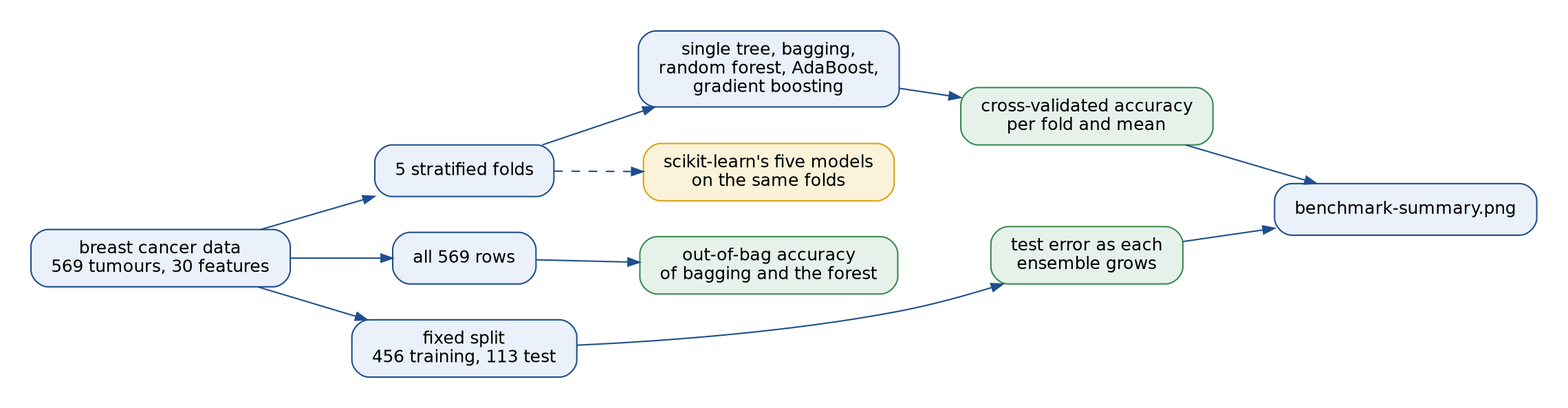
It scores every model by five-fold stratified cross-validation on the same folds, compares the out-of-bag accuracy of bagging and the forest on all rows with their cross-validated accuracy, follows the test error of every ensemble as it grows on a fixed split into 456 training and 113 test rows, and finally runs scikit-learn's versions of the five models on the same folds. Options such as --seed, --folds, --trees, --rounds, --boosting-trees, --max-features and --learning-rate change the setup, --skip-sklearn leaves out the library run, and --figures sends the PNG to another folder so a custom run does not overwrite the one shown here. The default run takes about 20 seconds.

python machine-learning/ensembles/project/ensemble_benchmark.py
python machine-learning/ensembles/project/ensemble_benchmark.py --max-features 1 --skip-sklearn

With the defaults the cross-validated accuracies, with the standard deviation over the folds in brackets, are:

• single tree 0.9315 (0.0103),
• bagging 0.9526 (0.0118),
• random forest 0.9649 (0.0235),
• AdaBoost 0.9789 (0.0172),
• gradient boosting 0.9667 (0.0218).

Every ensemble beats the single tree, by two to five points, and the random forest beats bagging, as it should on data with many strong, redundant features. The out-of-bag accuracy on all rows is 0.9596 for bagging and 0.9561 for the forest, within a point of the cross-validated values, without any folds. On the fixed split the single tree's test error is 0.1150; after 200 trees bagging reaches 0.0708 and the forest 0.0442, AdaBoost reaches 0.0442 after 400 rounds and gradient boosting 0.0354 after 400 trees. The forest's out-of-bag error, computed from the training rows alone, is 0.0713 after 5 trees, 0.0442 after 10 and 0.0329 after 200. With 113 test rows one mistake is 0.0088, so differences of one or two rows mean little, and the fold standard deviations are as large as the gaps between the ensembles.

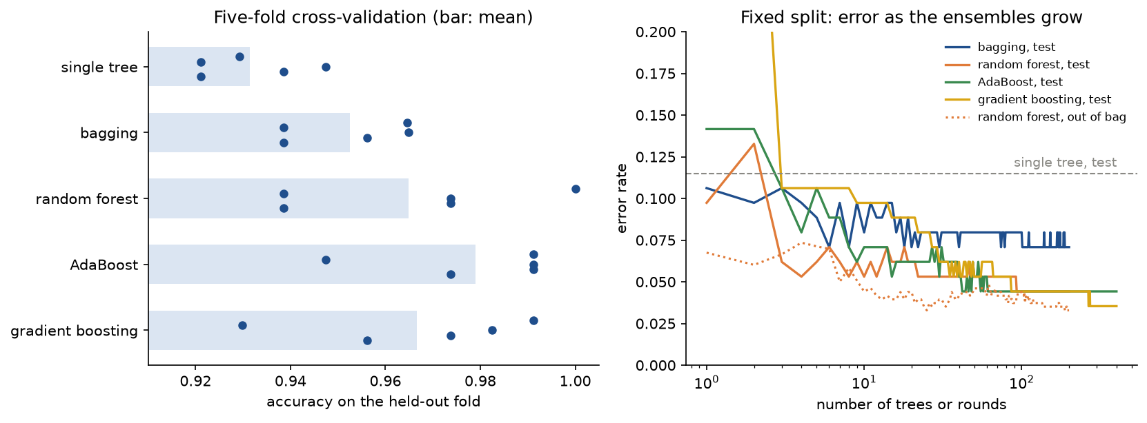
The fold dots show how much of the ranking is noise: each model's five folds spread over three to six points. On the right, every ensemble drops below the single tree within a few members. Gradient boosting starts above the top of the axis, at 0.3717, because its first two trees, small steps from the log-odds of the share of malignant tumours, still call every tumour benign; from the third tree on it falls with the others. scikit-learn's models on the same folds score 0.9350, 0.9544, 0.9596, 0.9684 and 0.9649, within about a point of ours everywhere; the largest gap, for AdaBoost, comes from the library choosing its stumps by Gini impurity rather than by weighted error.

The notebook ensembles.ipynb is a guided tour in the order of this page: averaging and the bootstrap, the AdaBoost worked example with its figure, resampling with both normalizations, the exponential-loss checks, gradient boosting by hand, a smaller tree-correlation experiment, the pitfalls, a short benchmark and the comparison with scikit-learn. The tests in tests check the worked examples value by value, the mathematical properties above and the agreement with scikit-learn, and run in a few seconds:

python -m pytest machine-learning/ensembles

Data: the Breast Cancer Wisconsin (Diagnostic) data were created by W. H. Wolberg, W. N. Street and O. L. Mangasarian (1995) and are distributed by the UCI Machine Learning Repository under the Creative Commons Attribution 4.0 licence. scikit-learn ships a copy as sklearn.datasets.load_breast_cancer, so nothing is downloaded. The target is recoded so that malignant is 1. The Friedman regression problem (J. H. Friedman, 1991) and every other data set here are synthetic and generated from fixed seeds.

In practice

scikit-learn has a counterpart for every model on this page, and with the same samples and settings it gives the same numbers. examples/compare_with_sklearn.py and tests/test_comparisons.py check:

• BaggingClassifier exposes the bootstrap samples it drew as estimators_samples_. On those samples, with depth-2 trees on synthetic data, our probabilities are identical to the library's, with a largest difference of 0, and both out-of-bag accuracies are 0.7667. With fully grown trees on the breast cancer split the test accuracies are 0.9292 (ours) and 0.9381, and the out-of-bag accuracies 0.9605 and 0.9583.
• RandomForestClassifier with max_features=None on the same samples is bagging and matches ours exactly. With feature sampling the two draw different features, so they agree on average: over five seeds of 100-tree forests the test accuracy is 0.9451 ± 0.0066 for ours and 0.9398 ± 0.0103 for the library, and the out-of-bag accuracy 0.9627 ± 0.0048 and 0.9645 ± 0.0043.
• AdaBoostClassifier runs SAMME, which for two classes is AdaBoost.M1, with Gini stumps. With criterion="gini" our 300 rounds on the breast cancer split agree with it to 2.1 × 10⁻¹⁴ in the errors and 9.6 × 10⁻¹⁴ in the vote weights, with identical test predictions and accuracy 0.9381. Stumps chosen by weighted error reach 0.9558 on the same split.
• GradientBoostingRegressor with 300 depth-3 trees and ν = 0.1 on 500 Friedman rows agrees with ours at every stage on the training rows to within 1.4 × 10⁻¹⁴; with at least ten rows per leaf, predictions on new rows agree to 1.8 × 10⁻¹⁴ and both test errors are 2.3468.
• GradientBoostingClassifier with stumps on synthetic data gives the same probabilities as ours to 2.2 × 10⁻¹⁶, which confirms the Newton leaves. With its default depth-3 trees on the breast cancer split our test accuracy is 0.9558 and the library's 0.9469, and the predictions agree on 112 of 113 rows.
• StackingClassifier with a forest, AdaBoost and 15 nearest neighbours and a logistic meta-learner with C = 100 builds the out-of-fold predictions itself and reaches test accuracy 0.9469.

The only disagreements come from exact ties between candidate splits. With bootstrap counts as weights, Gini scores are ratios of small integers, and features such as radius, perimeter and area sort the rows almost identically, so two different splits often score exactly the same. scikit-learn visits the features in a random order and keeps the first best split it meets; we keep the lowest feature index. The rate at which our trees differ from scikit-learn's equals the rate at which scikit-learn's differ from themselves under another seed: on the breast cancer split our bagged trees agree with the library's on 96.18 % of test predictions, and the library's trees with refits under other seeds on 96.26 %, while the two forests agree on 99.12 %. The same happens in gradient boosting with single-row leaves: on new rows our predictions differ from the library's by up to 0.90, and two library runs that differ only in random_state differ by up to 0.61, while the test errors, 2.4481 and 2.4573, are as close as two library runs. The first tree of a log-loss model fits residuals that take only two values, so ties are frequent there too, which is why the exact classifier comparison uses stumps. scikit-learn converts features to 32-bit floats before growing trees, so the exact comparisons use data that are representable in 32 bits.

When to use which:

• A random forest is the safest default for tabular data: few settings matter, it rarely overfits as trees are added, and the out-of-bag error comes free. RandomForestClassifier and ExtraTreesClassifier, which also randomizes the thresholds, are fast and parallel.
• Gradient-boosted trees are usually the most accurate choice on tabular data when tuned, with a small learning rate, shallow trees and early stopping on a validation set. Use HistGradientBoostingClassifier or HistGradientBoostingRegressor in scikit-learn, or XGBoost, LightGBM or CatBoost; they use second-order leaf values, and most of them bin the features into histograms for speed. They are a common choice for detection problems on tabular records, such as flagging network intrusions from flow features; there the rare classes are handled with class weights or with resampling applied inside the training folds only (Data leakage and pitfalls), and the result is judged with per-class metrics rather than accuracy (Evaluation metrics).
• AdaBoost with stumps is simple and strong on clean data, as in the benchmark above, but sensitive to label noise.
• Bagging helps any unstable learner, not only trees; BaggingClassifier takes any estimator. It does little for stable learners such as linear models or k-nearest neighbours with large k.
• Stacking squeezes out the last percent when several different, comparably good models exist; it costs training time and makes the system harder to maintain. StackingClassifier builds the out-of-fold predictions itself.
• The Isolation Forest of Anomaly detection is another averaging ensemble of randomized trees, built for scoring outliers rather than predicting labels.
• Use the from-scratch versions here to see every weight and every split; use the library versions for anything else, since they are faster, parallel and maintained.

Pitfalls

• Normalizing the AdaBoost weights over the sampled rows only. The weights must be renormalized over all n rows after every round, and every row must be updated by whether it is classified correctly, drawn or not. Rescaling only the drawn rows to their old sum over the sample, as some write-ups do, breaks the sum: 1.0692 after the first round of the worked example. On the breast cancer split the total climbs to 1.6522; errors computed against it are inflated by the same factor, the vote weights shrink, and after 14 rounds no draw gives an error below one half, so boosting stops with test accuracy 0.9115, against 0.9558 for 300 correctly normalized rounds (examples/common_mistakes.py). A one-line check catches it: assert that the weights sum to one and that the last stump has weighted error exactly one half after each update, as tests/test_adaboost.py does. Code that samples with numpy.random.Generator.choice refuses weights that do not sum to one, which tempts implementers to renormalize only for the draw and hide the problem.

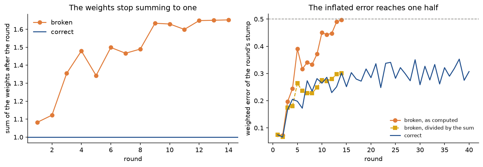
The inflated error, not the model, reaches one half: divided by the drifting sum, the broken run's errors look like the correct run's.

• Computing a resampled round's error on the sample. The error must use all training rows with their weights. In the worked example row 2 is never drawn in round 1, so the error on the sample is 0.1 instead of 0.2 and the vote weight would be ln 9 = 2.1972 instead of ln 4 = 1.3863 (tests/test_pitfalls.py).
• Mixing two forms of the vote weight. The vote weight, half of it, or the same expression with another logarithm base all give the same classifier, because they scale every vote equally; tests/test_pitfalls.py checks it with base-10 logarithms. The weight update, however, must multiply the mistakes by exactly (1 - ε)/ε relative to the correct rows. In round 1 of the worked example the correct factor leaves the mistakes with half the weight; e to the power α/2 leaves them 0.3333, and e to the power of a base-10 α leaves them 0.3134 (examples/common_mistakes.py).
• Calling boosting bootstrap aggregation. Bagging is short for bootstrap aggregating. Boosting reweights the data sequentially and does not need bootstrap samples at all.
• Drawing the random feature subset once per tree. A random forest draws m candidate features at every split. Drawing them once per tree and growing the whole tree on them is the random subspace method; with small m many trees never see the informative features. Out-of-bag accuracy on the breast cancer data with 100 trees and m = 1 is 0.9631 per split and 0.9016 per tree (examples/forest_experiments.py).
• Assuming more decorrelation is always better. Lower m lowers ρ but raises the bias. On the Friedman problem, where half the features are noise, the forest error is 12.847 with m = 1 and 5.828 with m = 10 (How it works, Random forests). Treat m as a setting to tune, for instance by out-of-bag error.
• Assuming forests take a majority vote. scikit-learn's forests average probabilities. The two rules coincide for fully grown trees and differ only for shallow ones: with depth-2 trees one of 113 test predictions on the breast cancer split changes, and the soft vote is right there (examples/forest_experiments.py).
• Reading the out-of-bag error of a small forest as the forest's error. Each row's out-of-bag prediction uses only about 37 % of the trees, and a row has no out-of-bag tree at all with probability about 0.632 to the power B. The forest's out-of-bag error on the project's split is 0.0713 after 5 trees and 0.0329 after 200.
• Boosting noisy labels. The exponential loss grows exponentially with the negative margin, so AdaBoost keeps raising the weight of rows it cannot fit. With 15 % of the breast cancer training labels flipped, the 68 flipped rows end up with 0.4251 of the weight, and the test error of AdaBoost rises from 0.1062 after 10 rounds to 0.1593 after 400, while a random forest goes from 0.0442 on clean labels to only 0.0619 (examples/common_mistakes.py). Prefer forests, gradient boosting with the logistic or a robust loss, or early stopping when labels are noisy.
• Choosing the number of boosting rounds on the test set, or not at all. Training error falls to zero whatever the learning rate, and test error has a minimum: after 5 trees for ν = 1 and after 353 for ν = 0.1 on the Friedman problem. Pick the number of rounds on a validation split or by cross-validation, and keep the test set for the final number.
• Trusting impurity importance. It is computed on the training rows and rewards features with many split points. In examples/common_mistakes.py the label depends only on a binary feature, which agrees with it three times in four, yet a forest of fully grown trees gives a continuous noise feature the larger impurity importance, 0.465 against 0.233; permutation importance on fresh rows gives 0.171 to the real feature and -0.012 to the noise. Larger leaves (at least ten rows) reduce the bias, to 0.565 against 0.224. Permutation importance has its own blind spot: correlated features share credit, and on the breast cancer data no single feature exceeds 0.0080.
• Stacking on in-sample predictions. On their own training rows a forest and a 100-round AdaBoost look nearly perfect, so a logistic meta-learner fitted to those predictions gives the forest the weight 11.52 and the 15-nearest-neighbour model, the best of the three on the test rows (0.9646), only 1.03. With out-of-fold predictions from five folds the weights become 1.52 for the forest, 11.07 for AdaBoost and 3.84 for the neighbours, and the test log loss improves from 0.2235 to 0.1545, although one more test row ends up on the wrong side, 0.9469 against 0.9558 in accuracy (examples/common_mistakes.py).
• Expecting two tree implementations to agree split for split. Exact ties between candidate splits are common with integer counts, redundant features and two-valued residuals, and every implementation breaks them its own way. Compare predictions on the training rows, aggregate accuracy, or shallow trees on continuous data, as the tests do, and remember that scikit-learn rounds features to 32-bit floats.

Further reading

• L. Breiman, "Bagging predictors", Machine Learning 24(2), 123-140, 1996.
• L. Breiman, "Random forests", Machine Learning 45(1), 5-32, 2001. Defines the forest, its out-of-bag estimates and the bound in terms of strength and correlation.
• T. K. Ho, "The random subspace method for constructing decision forests", IEEE Transactions on Pattern Analysis and Machine Intelligence 20(8), 832-844, 1998.
• Y. Freund and R. E. Schapire, "Experiments with a new boosting algorithm", Proceedings of ICML, 148-156, 1996. AdaBoost.M1, and boosting by resampling against reweighting.
• Y. Freund and R. E. Schapire, "A decision-theoretic generalization of on-line learning and an application to boosting", Journal of Computer and System Sciences 55(1), 119-139, 1997.
• J. Friedman, T. Hastie and R. Tibshirani, "Additive logistic regression: a statistical view of boosting", The Annals of Statistics 28(2), 337-407, 2000. AdaBoost as stagewise minimization of the exponential loss.
• J. H. Friedman, "Greedy function approximation: a gradient boosting machine", The Annals of Statistics 29(5), 1189-1232, 2001, and "Stochastic gradient boosting", Computational Statistics and Data Analysis 38(4), 367-378, 2002.
• J. H. Friedman, "Multivariate adaptive regression splines", The Annals of Statistics 19(1), 1-67, 1991. The source of the Friedman regression problem.
• T. Chen and C. Guestrin, "XGBoost: a scalable tree boosting system", Proceedings of KDD, 785-794, 2016.
• J. Zhu, H. Zou, S. Rosset and T. Hastie, "Multi-class AdaBoost", Statistics and Its Interface 2(3), 349-360, 2009. The SAMME algorithm.
• D. H. Wolpert, "Stacked generalization", Neural Networks 5(2), 241-259, 1992.
• C. Strobl, A.-L. Boulesteix, A. Zeileis and T. Hothorn, "Bias in random forest variable importance measures: illustrations, sources and a solution", BMC Bioinformatics 8, 25, 2007.
• B. Efron and R. J. Tibshirani, An Introduction to the Bootstrap, Chapman and Hall, 1993.
• T. Hastie, R. Tibshirani and J. Friedman, The Elements of Statistical Learning, second edition, Springer, 2009, chapters 8, 10, 15 and 16.
• R. E. Schapire and Y. Freund, Boosting: Foundations and Algorithms, MIT Press, 2012.
• W. N. Street, W. H. Wolberg and O. L. Mangasarian, "Nuclear feature extraction for breast tumor diagnosis", Proceedings of SPIE 1905, 861-870, 1993. The features of the breast cancer data.