Linear algebra for machine learning

Almost every model in this handbook stores its data as a matrix with one example per row, and most of them use a small set of ideas from linear algebra. Linear regression projects a vector of targets onto the space spanned by the feature columns. PCA finds the axes along which a cloud of points spreads most, which are eigenvectors of its covariance matrix and singular vectors of the data. A neural network layer is a matrix acting on a vector. This page treats those ideas as they are used: vectors and angles, matrices as maps of space, linear systems and their subspaces, orthogonal projection and least squares, orthonormal bases with Gram-Schmidt and QR, eigenvalues and the spectral theorem, power iteration, the singular value decomposition, the Eckart-Young theorem behind low-rank approximation and PCA, and the condition number that decides how many digits a computation keeps. One four-point data set is carried through all of it by hand, every routine is then written from scratch in NumPy and checked against numpy.linalg, and a sample project compresses an image with the truncated SVD. Afterwards you will be able to derive the normal equations from a picture, compute an eigen-decomposition and an SVD on paper, explain why PCA is an SVD of centred data, and tell a numerically sound least-squares solver from one that throws away half the digits.

To run the code in this topic, install the base group; the ml group adds the comparisons with scikit-learn and SciPy, and the vision group adds the optional photograph in the sample project.

Intuition

A vector is a list of numbers that can be read as a point or an arrow: one example's features, one word's embedding, one column of a data table. The dot product of two vectors measures how far they point the same way. Divided by both lengths it is the cosine of the angle between them, the cosine similarity used to compare embeddings.

A matrix is a machine that moves every point of space at once, and it does so linearly: straight lines stay straight, parallel lines stay parallel and the origin stays put. Such a map is fixed by where it sends the basis vectors, and those images are the columns of the matrix.

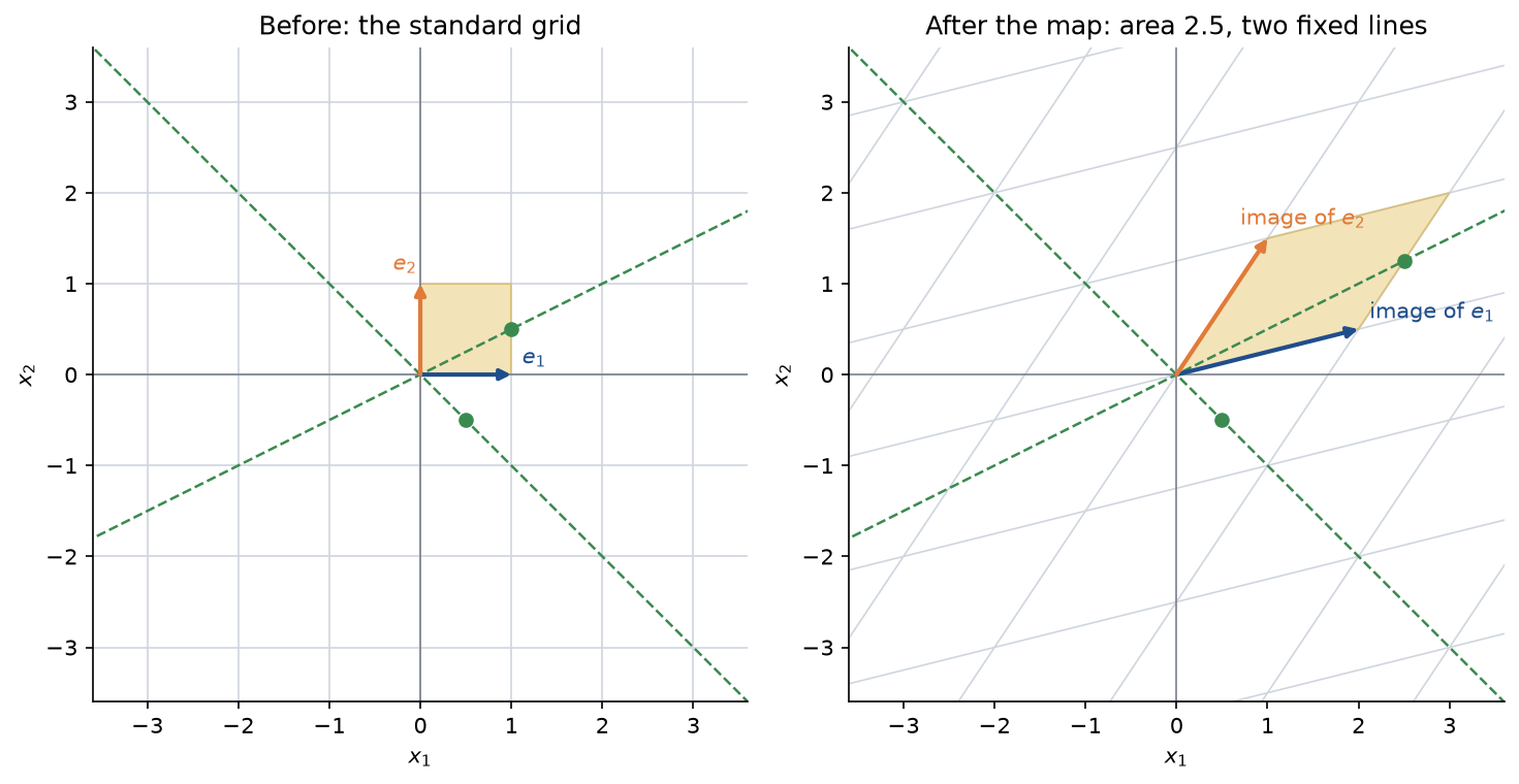
The figure shows the matrix M with rows (2, 1) and (0.5, 1.5) acting on the plane. The unit square becomes a parallelogram whose area, 2.5, is the determinant. The two dashed lines are mapped onto themselves: points on them are only stretched, the dot on the line through (2, 1) moves outwards by a factor of 2.5 and the dot on the line through (1, -1) does not move at all. These directions are the eigenvectors.

Doing one map after another is again a linear map, and its matrix is the product of the two matrices. Order matters, as the letter F shows.

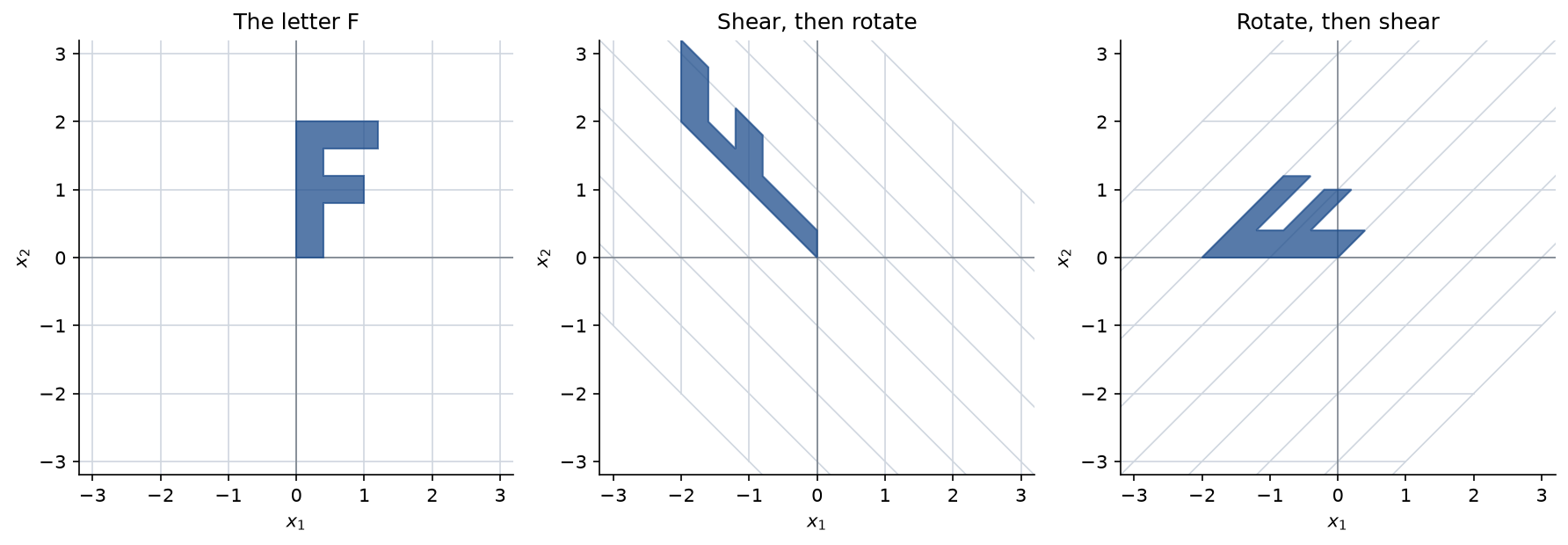
Shearing first and rotating second is not the same as rotating first and shearing second, so the two products of the matrices differ.

Least squares is a question about distance. A linear model can only produce prediction vectors that are combinations of the feature columns. Those combinations form a flat subspace, the column space, and the target vector usually lies outside it. The best prediction is the point of the column space closest to the target, the foot of the perpendicular. Writing down "the error is perpendicular to every column" gives the normal equations directly, without calculus.

The singular value decomposition says that every matrix is a rotation, a stretch along the coordinate axes and another rotation (rotations may include a reflection). Keeping only the largest stretches gives the best low-rank approximation of the matrix, and applied to centred data, the directions of those stretches are the principal components.

The map shows how the sections below connect. Least squares can be reached in two ways, through the normal equations or through an orthonormal basis, and the dashed amber edge marks why the second is usually preferred: the normal equations square the condition number.

How it works

Notation

Vectors are columns. A data matrix holds one example per row, as in NumPy, scikit-learn and PyTorch. A matrix A has m rows and n columns, its column j is the vector aj and its entry in row i and column j is Aij. The formula images write indices as subscripts and the transpose as a superscript T; in the text, Aᵀ is the transpose of A, a1 and a2 are the first two columns, σ1 is the largest singular value, λ1 the largest eigenvalue, and q1, u1 and v1 the matching vectors. The column space of A is C(A), its null space N(A) and its rank r. The condition number is κ, and ε is machine epsilon, 2⁻⁵² or about 2.2 × 10⁻¹⁶ in double precision.

Vectors, dot products, norms and angles

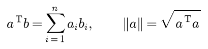
The dot product multiplies matching entries and adds them up, and the Euclidean length is the square root of the dot product of a vector with itself:

Two other norms appear often: the 1-norm, the sum of absolute values behind lasso penalties and absolute errors, and the max norm, the largest absolute entry. All three are special cases of the p-norm for p of at least 1:

The dot product carries the angle. Expanding the squared length of the difference of two vectors, and comparing the result with the law of cosines for the triangle with sides a, b and b - a, leaves the geometric meaning of the dot product:

In more than three dimensions the last line is the definition of the angle, and it needs the dot product to be no larger than the product of the lengths in absolute value, the Cauchy-Schwarz inequality. For any number t the squared length of b - t a is at least zero. The right side is smallest at the t shown in the second line, and substituting that value gives the inequality:

The minimizing t will return as the coefficient of a projection. Vectors with a zero dot product are orthogonal. The cosine of the angle, the dot product divided by both lengths, is the cosine similarity of text representations and retrieval.

For a = (1, 0, 1) and b = (2, 1, 2): the dot product is 4, b has 1-norm 5, length 3 and max norm 2, a has length √2 = 1.4142, the cosine of the angle is 4 / (3√2) = 0.9428 and the angle is 19.47 degrees.

Matrices as linear maps

A map f is linear when it respects combinations:

Writing x as a combination of the basis vectors ej shows that f(x) is the same combination of the vectors f(ej), so f is fixed by those n vectors. Put them side by side as the columns of A and the map becomes the matrix-vector product, which has two readings:

The first form is the column picture: A x is a combination of the columns with weights taken from x. The second is the row picture: output i is the dot product of row i with x. A fully connected layer in perceptrons and multilayer networks is a linear map followed by a shift.

For M in the figure, the first basis vector goes to (2, 0.5) and the second to (1, 1.5). The determinant of a 2 by 2 matrix is the signed area of the parallelogram spanned by its columns, so it is the factor by which the map scales every area:

For M that is 2 × 1.5 - 1 × 0.5 = 2.5. A negative determinant means the map flips orientation, and a zero determinant means the columns are dependent and the map flattens the plane onto a line or a point. In n dimensions the determinant scales volumes in the same way.

Matrix multiplication is composition

Applying B (k by n) and then A (m by k) is a linear map, so it has a matrix, and its column j is where ej ends up: A times column j of B. That is the definition of the product:

The inner sizes must agree, and the result is m by n. Several rules follow from composition without any index juggling:

• Composition of functions is associative. The two orders of evaluation can still cost very different amounts of arithmetic.
• It is not commutative. For the quarter turn R with rows (0, -1) and (1, 0) and the shear S with rows (1, 1) and (0, 1), the product RS has rows (0, -1) and (1, 1), but SR has rows (1, -1) and (1, 0).
• Area factors multiply, and undoing a composition undoes the last map first.

Linear systems, rank and the four subspaces

The system A x = b asks for weights x that combine the columns of A into b. It has a solution exactly when b lies in the column space. The directions that A flattens to zero form the null space:

Gaussian elimination answers both questions. Swapping rows, scaling a row and adding a multiple of one row to another do not change the solution set, and they reduce A to reduced row echelon form, where each nonzero row starts with a 1, a pivot, that is the only nonzero entry in its column. The number of pivots is the rank r. It equals the dimension of the column space and of the row space. Columns without a pivot correspond to free variables, and setting one free variable to 1, the others to 0 and reading the pivot variables off the reduced rows gives one basis vector of the null space per free column. Every column is either a pivot column or a free column, which is the rank-nullity theorem:

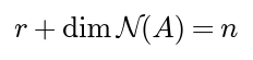
If one solution of A x = b is known, every solution is that one plus a null-space vector, so a solution is unique only when the null space holds the zero vector alone, that is when r = n. A square matrix is invertible exactly when r = n, which is when its determinant is not zero.

The matrix A with rows (1, 2, 1, 3), (2, 4, 0, 2) and (3, 6, 1, 5) has a third row equal to the sum of the first two. Its reduced form has rows (1, 2, 0, 1), (0, 0, 1, 2) and (0, 0, 0, 0), with pivots in columns 1 and 3, so r = 2. The free columns 2 and 4 give the null-space basis (-2, 1, 0, 0) and (-1, 0, -2, 1), and 2 + 2 = 4. The system is solvable exactly when b3 = b1 + b2: for b = (7, 8, 15) it is, for b = (1, 0, 0) it is not.

Two orthogonality facts complete the picture. If A x = 0 then x is orthogonal to every row of A, so the null space is orthogonal to the row space. Applied to Aᵀ, the left null space, the null space of Aᵀ, is orthogonal to the column space.

The diagram shows the four fundamental subspaces with their dimensions. A carries the row space one to one onto the column space and sends the null space to zero; Aᵀ does the same in the other direction. Least squares lives in the right-hand pair: the residual of a least-squares fit lies in the left null space.

Orthogonal projection

Projecting b onto the line through a means finding the multiple t a closest to b. The error b - t a must be perpendicular to a, which fixes t:

For the vectors above, p = (4 / 2)(1, 0, 1) = (2, 0, 2) and the error is (0, 1, 0), which is orthogonal to a.

Now project onto the column space of A, an m by n matrix with independent columns, so r = n. The projection is some combination A x̂, and the error b - A x̂ must be perpendicular to every column. Stacking these n conditions gives the normal equations, named because the error is normal (perpendicular) to the column space:

The matrix AᵀA is invertible when the columns are independent: if AᵀA x = 0, then xᵀAᵀA x, the squared length of A x, is 0, so A x = 0 and x = 0. The same argument shows that AᵀA has the same null space as A for any A. Hence:

Projecting twice changes nothing, the projection matrix is symmetric, its trace is n, and I - P projects onto the left null space. The projection is also the closest point of the column space. For any x, b - A x splits into the error e and A(x̂ - x), which lies in the column space and is therefore orthogonal to e, so Pythagoras applies:

Equality holds only at A x = A x̂, and taking x = 0 splits the squared length of b into those of p and e.

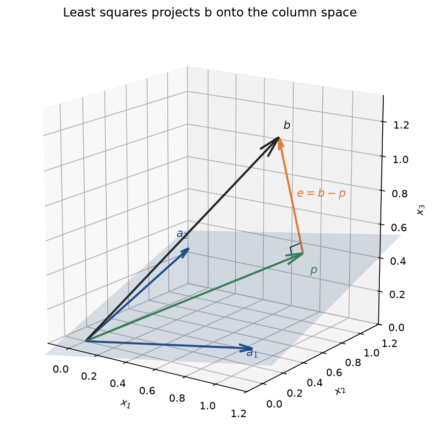
The picture shows the plane spanned by a1 = (1, 0.2, 0.1) and a2 = (0, 1, 0.3) and the target b = (0.7, 0.9, 1.1). The least-squares coefficients are (0.7294, 0.9745), the projection is p = (0.7294, 1.1204, 0.3653), the error e = (-0.0294, -0.2204, 0.7347) is perpendicular to both columns, and the squared lengths satisfy 2.5100 = 1.9208 + 0.5892.

Least squares as projection

A linear model predicts X w for coefficients w, and least squares chooses w to minimize the sum of squared residuals. As w varies, X w runs over the column space of X, a subspace with one coordinate per example. The best prediction is therefore the projection of y onto that column space, and the coefficients solve the normal equations; calculus, through the gradient in the second line, gives the same equations:

The geometry adds two facts calculus leaves implicit: the minimum exists, and it is unique exactly when the columns are independent. With a column of ones for the intercept, the residual is orthogonal to that column, so the residuals sum to zero.

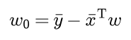
Centring removes the intercept from the algebra. Subtract the mean of each feature and of the target. The centred columns sum to zero, so they are orthogonal to the column of ones, and the design with raw features and a column of ones has the same column space as the one with centred features and a column of ones. Projection onto a space spanned by two orthogonal pieces is the sum of the two projections: onto the ones it is the mean target, and onto the centred columns it is X w with w from the centred normal equations. The intercept follows from the means x̄ of the features and ȳ of the target:

Linear regression builds on this with gradient descent, feature scaling and ridge regularization.

Orthonormal bases, Gram-Schmidt and QR

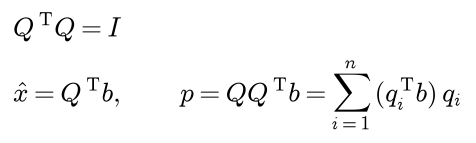
Vectors q1 to qn are orthonormal when each has length 1 and every two are perpendicular. As the columns of Q this reads QᵀQ = I, and projection then needs no system solving, because the normal equations collapse:

A square Q with orthonormal columns is an orthogonal matrix. Its inverse is its transpose, and it preserves lengths and angles because the squared length of Q x is xᵀQᵀQ x = xᵀx. Its determinant is 1 or -1, a rotation or a reflection.

Gram-Schmidt turns independent vectors a1 to an into orthonormal ones spanning the same spaces. Subtract from aj its projections onto the directions already found, then normalize:

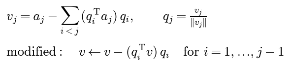
The modified variant subtracts the projections one at a time from the running vector. Because qi is orthogonal to the earlier directions, the coefficient taken from the running vector equals the one taken from aj in exact arithmetic, so the two variants agree on paper. In floating point they do not, as Pitfalls shows.

Read backwards, Gram-Schmidt writes each aj as a combination of q1 to qj, with the coefficients removed above the diagonal and the leftover lengths on it. In matrix form A = QR with R upper triangular and a positive diagonal, and least squares then avoids AᵀA altogether:

The triangular system is solved by back substitution from the last row up. In floating point, Qᵀb should be formed the way modified Gram-Schmidt would treat b as an extra column: take its coordinate along q1, remove that component, then take the coordinate along q2 of what is left, and so on. LAPACK, and so numpy.linalg.qr, computes QR with Householder reflections instead, which are orthogonal to working precision by construction.

Eigenvalues and eigenvectors

A nonzero vector q is an eigenvector of a square matrix A, with eigenvalue λ, when the map only stretches it by the factor λ. Then A - λI sends q to zero, so it is singular, and λ solves a polynomial equation of degree n, the characteristic equation:

In general the eigenvalues sum to the trace and multiply to the determinant. For M, λ² - 3.5λ + 2.5 = 0 gives λ = 2.5 and λ = 1. The null spaces of M - 2.5I and M - I are spanned by (2, 1) and (1, -1), the dashed lines in the grid figure. If A has n independent eigenvectors, collect them as the columns of E and the eigenvalues in the diagonal matrix Λ. Then AE = EΛ, so:

In the eigenvector coordinates the map is just a stretch along each axis, and powers become powers of numbers. For M, E has columns (2, 1) and (1, -1) and Λ holds 2.5 and 1. Not every matrix can be diagonalized like this. The shear S has the eigenvalue 1 twice but only the eigenvector direction (1, 0), and a rotation by 90 degrees has eigenvalues i and -i and no real eigenvectors at all.

Symmetric matrices and the spectral theorem

Symmetric matrices, equal to their transposes, are the ones machine learning meets most: covariance matrices, Gram matrices XᵀX, Hessians and kernel matrices. For them the eigenvalue problem behaves perfectly. The spectral theorem says that a real symmetric matrix has real eigenvalues and an orthonormal basis of eigenvectors:

Two parts of the proof are short. Real eigenvalues: if A q = λ q with a possibly complex q, multiplying by the conjugate transpose of q, and conjugating the result using that A is real and symmetric, gives the same number once with λ and once with its conjugate. Since the conjugate of q times q is a positive sum of squared magnitudes, λ equals its conjugate:

Orthogonal eigenvectors for distinct eigenvalues: move A across the dot product of two eigenvectors.

So (λ1 - λ2) q2ᵀq1 = 0, and q2ᵀq1 = 0 whenever the eigenvalues differ. For a repeated eigenvalue an orthonormal basis of its eigenvectors can still be chosen; the full proof is by induction on n (see Further reading). Writing x in the eigenvector basis turns every quadratic form into a weighted sum of eigenvalues:

Two consequences follow:

• A is positive semidefinite, with xᵀA x at least zero for all x, exactly when every eigenvalue is at least zero. Every Gram matrix is, since xᵀXᵀX x is the squared length of X x.
• The Rayleigh quotient is a weighted average of the eigenvalues. Its maximum over all nonzero x is λ1, attained at q1. Over the vectors orthogonal to q1 the maximum is λ2, attained at q2, and so on. This is the variance-maximization step of PCA.

Power iteration

Power iteration finds the eigenvalue of largest magnitude by applying the matrix again and again and rescaling:

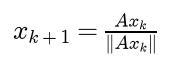
Suppose the eigenvalues are ordered by magnitude with a strict gap after the first, and write the start vector as a combination of eigenvectors with a nonzero coefficient c1 on q1. Then every power of A multiplies each coefficient by a power of its eigenvalue:

So the direction of the iterate approaches q1 or -q1, with an error that shrinks like the ratio of the second eigenvalue to the first, to the power k. For a symmetric matrix the Rayleigh quotient of the iterate converges to λ1 twice as fast, like the square of that ratio to the power k. A practical stopping rule is a small residual A x - λ x.

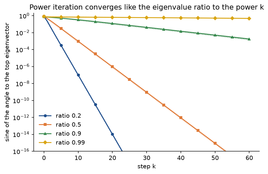
The plot runs power iteration on diagonal matrices with eigenvalues 1, the ratio and 0.1, starting from (1, 1, 1). Every curve follows its prediction, which is the whole story of power iteration: the gap between the top two eigenvalues sets the speed, and without a gap there is no convergence. To get further eigenpairs of a symmetric matrix, deflate:

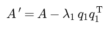
The deflated matrix has the same eigenvectors, with λ1 replaced by 0, so power iteration on it finds λ2. Libraries use the shifted QR algorithm or divide and conquer instead, but power iteration is still the method behind PageRank and inside randomized SVD.

The singular value decomposition

Every real m by n matrix A of rank r can be written as a sum of r rank-one pieces, each a singular value times the outer product of a left and a right singular vector, both sets orthonormal:

The decomposition follows from the spectral theorem. AᵀA is symmetric and positive semidefinite, so it has orthonormal eigenvectors v1 to vn with eigenvalues σ1² to σn², all at least zero. Its rank is r because it has the null space of A, so exactly r eigenvalues are positive. For those, define ui as A vi divided by σi. These are orthonormal, by the second line below, and since the vi form an orthonormal basis, inserting the identity as the sum of the products vi viᵀ gives the decomposition in the third:

For i beyond r, A vi has squared length viᵀAᵀA vi = 0, which is why those terms vanish. Likewise AAᵀ ui = σi² ui, so the ui are eigenvectors of AAᵀ. The SVD also hands over bases of all four subspaces: u1 to ur span the column space, v1 to vr the row space, the remaining v vectors the null space and the remaining u vectors the left null space. Geometrically, A maps the unit sphere onto an ellipsoid with semi-axes σi ui, so the largest stretch is σ1:

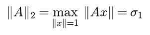
This largest stretch is the spectral norm, the size of a matrix that matters when errors are amplified. The figure below shows the stretching for M.

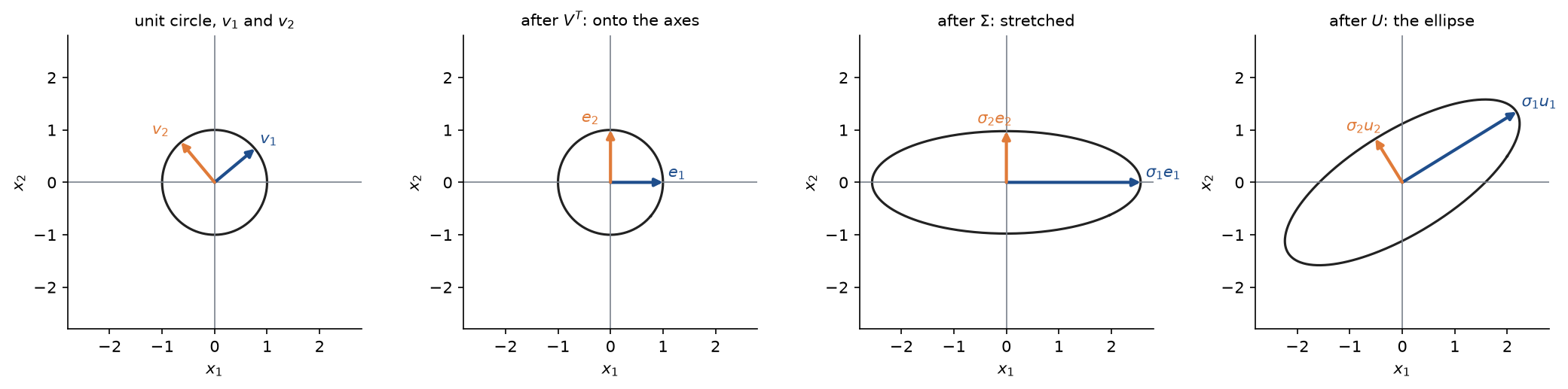
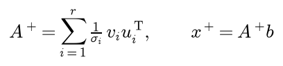
The four panels follow the unit circle through the three factors of M: a rotation, a stretch along the axes and another rotation. The pseudo-inverse inverts each stretch that is not zero and solves least squares in general. The solution it gives minimizes the residual and, among all minimizers, has the smallest length; for independent columns it equals the normal-equations solution:

Singular values are not eigenvalues except for symmetric positive semidefinite matrices. For M, MᵀM has rows (4.25, 2.75) and (2.75, 3.25) and eigenvalues 6.5451 and 0.9549, so σ1 = 2.5583 and σ2 = 0.9772, while the eigenvalues of M are 2.5 and 1. Both products equal the absolute determinant, 2.5.

Low-rank approximation and the Eckart-Young theorem

The Frobenius norm, the square root of the sum of squared entries, is also the square root of the sum of squared singular values:

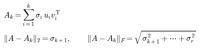
Truncating the sum after k terms gives a matrix of rank k, and the errors of the truncation follow at once, because what is left over is the sum of the discarded terms:

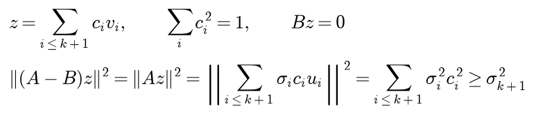
The Eckart-Young theorem says that no matrix B of rank at most k does better, in either norm. The proof for the spectral norm counts dimensions. The null space of B has dimension at least n - k, and the span of v1 to vk+1 has dimension k + 1. Their dimensions add up to more than n, so they share a unit vector z, on which B gives zero and A stretches by at least σk+1:

For the Frobenius norm, Weyl's inequality for singular values, applied with j = k + 1 where the singular value of B is zero, gives one inequality per singular value of A:

Squaring and summing over i shows that the squared Frobenius norm of A - B is at least the sum of the squared singular values of A beyond the k-th. The sample project below uses this theorem on an image: keeping 20 of the 192 singular triplets of a 192 by 256 test image stores 18 % of the numbers and leaves a relative error of 0.0455, exactly the value the discarded singular values predict.

From the SVD to PCA

Let the raw data have m examples of n features, and let X be the centred data matrix. The sample covariance matrix is XᵀX divided by m - 1. Project the data onto a unit direction w. The scores X w have mean zero because X is centred, and their sample variance is a Rayleigh quotient of the covariance:

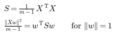
The direction of largest variance is therefore the top eigenvector of S, the next direction, orthogonal to the first, is the second eigenvector, and so on. These are the principal components, and the eigenvalues are the variances along them. The SVD of the centred data gives everything at once:

So the principal directions are the right singular vectors, the variances are the squared singular values divided by m - 1, and the scores are UΣ. Their covariance is diagonal, so the scores are uncorrelated. Keeping k components reconstructs the centred data as its best rank-k approximation, and the squared error is exactly the discarded variance times m - 1:

Maximizing the variance kept and minimizing the reconstruction error are the same problem.

The diagram is the whole of PCA as code. Libraries compute it from the SVD of X rather than the eigen-decomposition of S, for two reasons: forming XᵀX squares the condition number, as the next section shows, and the SVD never builds an n by n matrix when n is large. Dimensionality reduction applies PCA to real data and compares it with t-SNE and UMAP.

Conditioning

The condition number says how much a matrix can amplify relative errors. Let A be square and invertible, and perturb the right-hand side of A x = b. The change δx is A⁻¹ times the change δb, whose largest stretch is 1 / σn, and b itself is at most σ1 times as long as x. Multiplying the two inequalities gives the bound:

Equality holds when b points along u1 and δb along un. Every number stored in double precision carries a relative error of up to ε / 2, so even a perfect algorithm can return a solution with a relative error near κε. A computation loses about log₁₀ κ of its roughly 16 significant digits. For a matrix with independent columns, σ1 / σn plays the same role in least squares. Forming the normal equations squares it, because AᵀA has the squared singular values:

Solving the normal equations therefore loses about twice as many digits, whatever solver is used afterwards. QR with Householder reflections, modified Gram-Schmidt with the right-hand side treated as an extra column, and SVD-based solvers work with A itself and, when the residual is small, lose only about log₁₀ κ digits. (In general the sensitivity of least squares has a κ² term proportional to the residual, so a large residual on an ill-conditioned problem hurts every method.) Remedies, in order of preference: centre and scale the features, use an orthogonal basis such as orthogonal polynomials, and regularize. Ridge regression adds α times the identity to AᵀA, which lifts every squared singular value by α:

The smallest squared singular values gain the most, so even a small α shrinks a huge condition number dramatically, at the price of a small bias in the coefficients.

Worked example

Four observations of two features and one target:

• observation 1: features (2, 2), target 1
• observation 2: features (4, 2), target 3
• observation 3: features (7, 3), target 9
• observation 4: features (7, 5), target 11

The feature means are 5 and 3 and the mean target is 6. Every value below is computed in double precision and rounded to four decimals for display; where exact fractions are simple they are given as well.

Centring and the four subspaces

Subtracting the means gives the centred data matrix X with rows (-3, -1), (-1, -1), (2, 0) and (2, 2), and the centred targets y = (-5, -3, 3, 5).

The columns of X are independent, so r = 2, the null space holds only the zero vector and the column space is a plane in four dimensions. The left null space has dimension 4 - 2 = 2. Both columns sum to zero, so it contains the vector of ones. It also contains g = (-3, 5, -3, 1), since the first column gives 9 - 5 - 6 + 2 = 0, the second gives 3 - 5 + 0 + 2 = 0, and g is orthogonal to the ones as well. So the ones and g span the left null space. The residual of the regression with intercept is orthogonal to the ones and to both columns, so it must be a multiple of g.

Projection by the normal equations

The Gram matrix XᵀX has rows (18, 8) and (8, 6), and Xᵀy = (15 + 3 + 6 + 10, 5 + 3 + 0 + 10) = (34, 18). The determinant is 18 × 6 - 8 × 8 = 44, so the inverse of XᵀX is 1/44 times the matrix with rows (6, -8) and (-8, 18), and

• w1 = (6 × 34 - 8 × 18) / 44 = 60 / 44 = 15/11 = 1.3636,
• w2 = (-8 × 34 + 18 × 18) / 44 = 52 / 44 = 13/11 = 1.1818.

The projection of y onto the column space is p = X w = (-58, -28, 30, 56) / 11 = (-5.2727, -2.5455, 2.7273, 5.0909), and the residual is e = y - p = (3, -5, 3, -1) / 11 = (0.2727, -0.4545, 0.2727, -0.0909). As predicted, e = -g / 11. It is orthogonal to both columns: (-9 + 5 + 6 - 2) / 11 = 0 and (-3 + 5 + 0 - 2) / 11 = 0. Pythagoras holds: the squared length of y is 68, that of p is 8184/121 = 67.6364 and that of e is 4/11 = 0.3636. The fraction of the target's variation explained is 1 - 0.3636 / 68 = 0.9947. In the raw units the intercept is 6 - (5 × 15 + 3 × 13) / 11 = -48/11 = -4.3636, so the fitted model predicts -4.3636 + 1.3636 times the first feature + 1.1818 times the second. Least squares on the raw features with a column of ones gives exactly these three numbers.

The same projection by Gram-Schmidt and QR

The first column has length r11 = √18 = 4.2426, so q1 = (-3, -1, 2, 2) / √18 = (-0.7071, -0.2357, 0.4714, 0.4714). The second column a2 has component r12 = q1ᵀa2 = 8 / √18 = 1.8856 along q1. Subtracting it leaves v2 = a2 - (8/18) a1 = (3, -5, -8, 10) / 9, with length r22 = √198 / 9 = √22 / 3 = 1.5635, so q2 = (3, -5, -8, 10) / √198 = (0.2132, -0.3553, -0.5685, 0.7107). Together:

• Q has rows (-0.7071, 0.2132), (-0.2357, -0.3553), (0.4714, -0.5685) and (0.4714, 0.7107).
• R has rows (4.2426, 1.8856) and (0, 1.5635).

As a check, r11² r22² = 18 × 22/9 = 44, the determinant of XᵀX. Then Qᵀy = (34/√18, 26/√198) = (8.0139, 1.8477), and back substitution gives w2 = (26/√198) / (√198/9) = 234/198 = 13/11 and w1 = (34 - 8 × 13/11) / 18 = 15/11, the same coefficients without ever forming XᵀX. With the rounded values, w1 = (8.0139 - 1.8856 × 1.1818) / 4.2426 comes out as 1.3637, one unit off in the last digit.

Eigen-decomposition of the Gram matrix

The characteristic equation of XᵀX is λ² - 24λ + 44 = (λ - 22)(λ - 2) = 0, so λ1 = 22 and λ2 = 2, with trace 24 and determinant 44 as they must be. The null space of XᵀX - 22I, with rows (-4, 8) and (8, -16), is spanned by (2, 1), and that of XᵀX - 2I, with rows (16, 8) and (8, 4), by (-1, 2). The two are orthogonal, as the spectral theorem promises. Normalized, with the sign convention of the code (the largest entry in magnitude is positive), q1 = (2, 1)/√5 = (0.8944, 0.4472) and q2 = (-1, 2)/√5 = (-0.4472, 0.8944). Rebuilding the matrix from them, 22/5 times the matrix with rows (4, 2) and (2, 1) plus 2/5 times the matrix with rows (1, -2) and (-2, 4) gives back the rows (18, 8) and (8, 6).

Power iteration by hand

Start from x0 = (1, 0) and multiply by XᵀX, dropping common factors since only the direction matters. The ratio of the two entries should approach 2, the slope of q1:

• Step 0: (1, 0), Rayleigh quotient 18.
• Step 1: (18, 8), proportional to (9, 4); normalized (0.9138, 0.4061); ratio 2.25, distance from 2 equal to 0.25; Rayleigh quotient 2130/97 = 21.9588.
• Step 2: (194, 96), proportional to (97, 48); normalized (0.8963, 0.4435); ratio 2.0208, distance 0.0208; Rayleigh quotient 21.9997.
• Step 3: (2130, 1064), proportional to (1065, 532); normalized (0.8946, 0.4469); ratio 2.0019, distance 0.0019; Rayleigh quotient 22.0000.

The distance from 2 shrinks by factors of 12 and 11.08, approaching λ1/λ2 = 11 as the analysis predicts, and the Rayleigh quotient converges to 22 even faster. Continued in integers for two more steps, (11713, 5856) and (128841, 64420), the shrink factors are 11.01 and 11.00.

The SVD and the rank-one approximation

The singular values of X are the square roots of the eigenvalues of XᵀX, σ1 = √22 = 4.6904 and σ2 = √2 = 1.4142, and the right singular vectors are q1 and q2. The left singular vectors follow from ui = X vi / σi:

• X v1 = (-7, -3, 4, 6)/√5, so u1 = (-7, -3, 4, 6)/√110 = (-0.6674, -0.2860, 0.3814, 0.5721).
• X v2 = (1, -1, -2, 2)/√5, so u2 = (1, -1, -2, 2)/√10 = (0.3162, -0.3162, -0.6325, 0.6325).

They are orthogonal: -7 + 3 - 8 + 12 = 0. The least-squares coefficients come out a third time through the pseudo-inverse. Uᵀy = (86/√110, 2/√10) = (8.1998, 0.6325); dividing by the singular values gives (1.7482, 0.4472), and w = 1.7482 v1 + 0.4472 v2 = (1.5636 - 0.2000, 0.7818 + 0.4000) = (1.3636, 1.1818).

The rank-one approximation keeps the first term, σ1 u1 v1ᵀ, the outer product of (-7, -3, 4, 6) and (2, 1) divided by 5, with rows (-2.8, -1.4), (-1.2, -0.6), (1.6, 0.8) and (2.4, 1.2). The remainder is σ2 u2 v2ᵀ, with rows (-0.2, 0.4), (0.2, -0.4), (0.4, -0.8) and (-0.4, 0.8). Its Frobenius norm is the square root of 0.04 + 0.16 + 0.04 + 0.16 + 0.16 + 0.64 + 0.16 + 0.64 = 2, which is √2 = 1.4142 = σ2. Its spectral norm is also σ2, because the remainder is a single rank-one term. By Eckart-Young no rank-one matrix comes closer to X.

PCA

The sample covariance is XᵀX / 3, with rows (6, 2.6667) and (2.6667, 2), and total variance 6 + 2 = 8. The principal directions are v1 = (0.8944, 0.4472) and v2 = (-0.4472, 0.8944), with variances 22/3 = 7.3333 and 2/3 = 0.6667, so the first component explains 22/24 = 0.9167 of the variance. The scores UΣ = X V are (-3.1305, -1.3416, 1.7889, 2.6833) on the first component and (0.4472, -0.4472, -0.8944, 0.8944) on the second. Adding the means back to the rows of the rank-one approximation gives the points projected onto the first axis: (2.2, 1.6), (3.8, 2.4), (6.6, 3.8) and (7.4, 4.2). Their squared distances from the data sum to σ2² = 2, which is (m - 1) λ2 = 3 × 0.6667, the discarded variance.

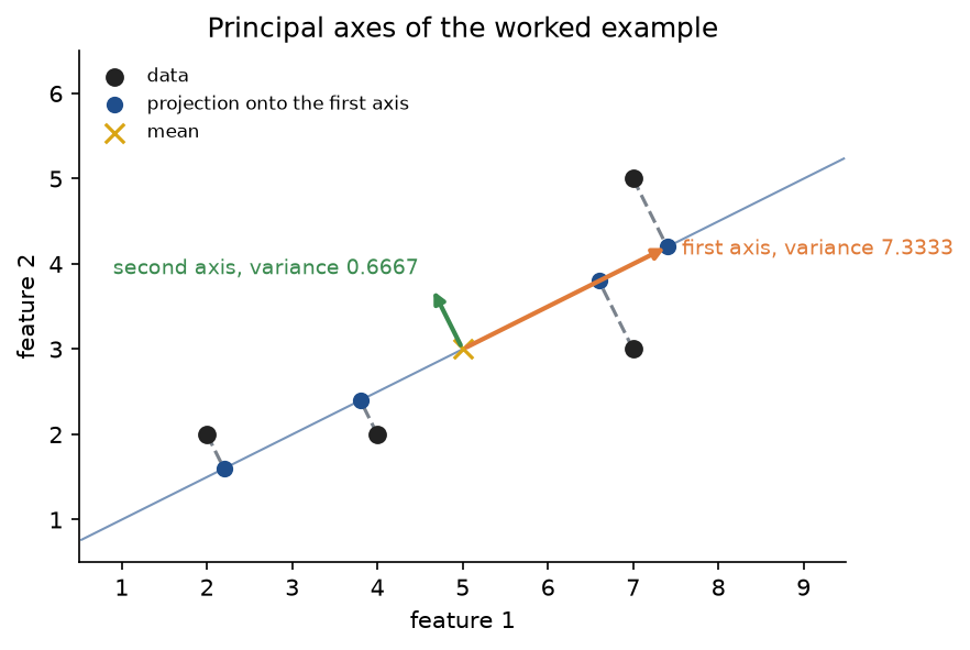
The dashed lines are the errors of the rank-one approximation. Each runs parallel to the second axis, because projecting onto the first axis removes exactly the second component.

Conditioning

The condition number of X is σ1/σ2 = √11 = 3.3166, and that of XᵀX is 22/2 = 11, the square. With such a small condition number every method on this page gives the same coefficients to 15 digits; Pitfalls shows what happens when κ grows.

Every number in this section is asserted by tests/test_trace.py and printed by examples/worked_example.py.

The code

The package linear_algebra_for_ml is plain NumPy, split into one module per idea. It uses array arithmetic and the @ product, but every factorization, solver and eigenvalue routine is written out. scikit-learn and SciPy are imported only inside the functions of comparisons.py, and scikit-image only when the sample project is asked for the photograph.

• arrays.py holds the Array type and the checks that turn inputs into vectors, matrices, square and symmetric matrices.
• vectors.py holds dot, norm for any p of at least 1 and for infinity, angle, cosine_similarity and project_onto_line.
• maps.py holds rotation, shear and scaling, matvec as a combination of columns and matmul as composition.
• elimination.py holds reduced_row_echelon, rank, column_space_basis, null_space_basis, elimination with partial pivoting, back_substitution, solve_linear_system and determinant.
• orthogonal.py holds qr_decomposition with classical or modified Gram-Schmidt, gram_schmidt and orthogonal_coordinates, which forms Qᵀb one direction at a time.
• least_squares.py holds least_squares_normal, projection_matrix, project_onto_column_space and least_squares_qr.
• eigen.py holds the closed form for a symmetric 2 by 2 matrix, power_iteration with its full history and symmetric_eigen by power iteration with deflation.
• svd.py holds the SVD class, svd_via_eigen, solve_with_svd, low_rank_approximation, frobenius_norm, spectral_norm and condition_number.
• pca.py holds pca, which returns components as rows (the scikit-learn layout), variances, ratios and scores.
• datasets.py generates polynomial design matrices, latent-factor data, the test image and matrices with chosen singular values.
• trace.py holds worked_example, trace_worked_example, which keeps every quantity of the worked example, and integer_power_iteration; report.py prints them.
• stability.py and pitfalls.py hold the experiments behind Pitfalls, comparisons.py the agreement checks with the libraries and compression.py the computations of the sample project.
• plotting.py, geometry_plots.py, analysis_plots.py and compression_plots.py draw every figure in the handbook's four colours and save it reproducibly.

Modified Gram-Schmidt differs from the classical version in one expression, the vector the projection coefficient is taken from:

for j in range(columns):
    v = a[:, j].copy()
    for i in range(j):
        r[i, j] = q[:, i] @ (v if modified else a[:, j])
        v -= r[i, j] * q[:, i]
    r[j, j] = np.sqrt(v @ v)
    q[:, j] = v / r[j, j]

power_iteration stops when the residual is below tolerance times the Frobenius norm of the matrix. symmetric_eigen runs it from a random start, deflates and repeats; in exact arithmetic deflation alone would keep later iterates away from the eigenvectors already found, but rounding errors slowly bring those directions back, so they are projected out at every step. Eigenvalues of equal size, such as 3 and -3, raise an error instead of returning a wrong vector, and each eigenvector is flipped so that its largest entry is positive. svd_via_eigen applies symmetric_eigen to AᵀA (or to AAᵀ through the transpose when A is wide), takes square roots and forms ui = A vi / σi. Eigenvalues below the tolerance come back as zero, so singular values below roughly 10⁻⁶ σ1 are dropped: they cannot be recovered through AᵀA anyway, as Pitfalls shows.

The examples and the project import the package, so install the repository first as described in the main README. The examples each demonstrate one idea and run in a few seconds at most from the repository root:

• examples/worked_example.py prints every value of the worked example in the order above and the integer power iteration, and saves the principal-axes figure.
• examples/linear_maps.py covers vectors, the matrix M as a map with its eigenvectors and singular values, and composition, and saves the grid, letter and SVD figures.
• examples/subspaces_and_projection.py runs elimination on the rank-two matrix, decides solvability, projects onto a plane in three dimensions and saves the projection figure.
• examples/numerical_stability.py sweeps polynomial fits through every least-squares method, computes singular values through AᵀA, tests singularity with determinants and measures power iteration against the eigenvalue gap, and saves the stability and convergence figures.
• examples/common_mistakes.py demonstrates the eigh column order, PCA without centring, the broadcast residual, the two variance divisors, eigenvalues mistaken for singular values and the wrong covariance product.
• examples/compare_with_libraries.py compares every routine with numpy.linalg, PCA with scikit-learn and the null space with SciPy, and saves the PCA figure.

python foundations/linear-algebra-for-ml/examples/worked_example.py
python foundations/linear-algebra-for-ml/examples/linear_maps.py
python foundations/linear-algebra-for-ml/examples/subspaces_and_projection.py
python foundations/linear-algebra-for-ml/examples/numerical_stability.py
python foundations/linear-algebra-for-ml/examples/common_mistakes.py
python foundations/linear-algebra-for-ml/examples/compare_with_libraries.py

The sample project, project/svd_image_compression.py, compresses a grey-scale image with the truncated SVD. It loads a 192 by 256 test image (or, with --image camera, a 512 by 512 photograph, or any image file), takes the thin SVD with LAPACK and, before relying on it, recomputes the ten leading triplets with the from-scratch svd_via_eigen and stops if they disagree. It then keeps the top k triplets for ranks 1, 5, 10, 20 and 50, reports the numbers stored, the relative error, the Eckart-Young prediction of that error and the PSNR, finds the ranks that keep 99 % and 99.9 % of the energy and the smallest rank reaching 30 dB, and saves two figures. A rank-k approximation stores k columns of U, k rows of Vᵀ and k singular values, so it saves space only below the break-even rank:

Quality is measured by the peak signal-to-noise ratio, and Eckart-Young turns the discarded singular values directly into the mean squared error, so a rank can be chosen for a quality target without rebuilding a single image:

The diagram shows the two checks around the compression: the from-scratch triplets against the library before, and the measured error against Eckart-Young after. Options such as --image, --ranks, --panels, --energy and --psnr change the setup, and --figures sends the two PNGs to another folder so a custom run does not overwrite the ones shown here; the default run takes under a second.

python foundations/linear-algebra-for-ml/project/svd_image_compression.py
python foundations/linear-algebra-for-ml/project/svd_image_compression.py --image camera --ranks 1 5 10 20 50 100 --panels 10 50 100 --figures camera-figures

With the defaults the from-scratch singular values agree with LAPACK to a relative 8.0 × 10⁻¹⁶. The image has 49,152 pixels and the break-even rank is 109:

• rank 1 stores 449 numbers (0.91 % of the pixels), relative error 0.1981, 19.42 dB;
• rank 5 stores 2,245 numbers (4.57 %), relative error 0.0864, 26.63 dB;
• rank 10 stores 4,490 numbers (9.13 %), relative error 0.0577, 30.13 dB;
• rank 20 stores 8,980 numbers (18.27 %), relative error 0.0455, 32.19 dB;
• rank 50 stores 22,450 numbers (45.67 %), relative error 0.0306, 35.64 dB.

Every measured error equals its Eckart-Young prediction to all four digits. Rank 4 already keeps 99 % of the energy and rank 48 keeps 99.9 %, while 30 dB needs rank 10.

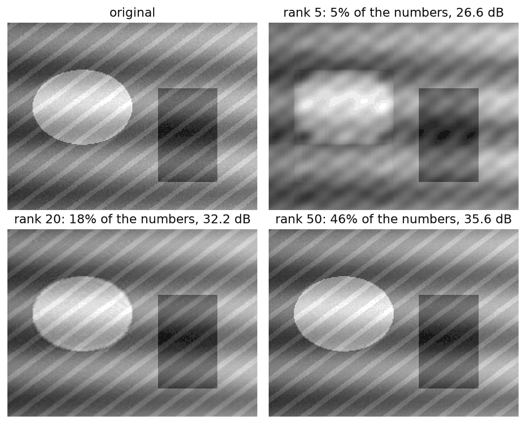
The panels show what rank means for a picture. The dark rectangle is an outer product of two indicator vectors, a rank-one matrix, so it is sharp from the start, and the horizontal gradient and the horizontal waves are rank-one patterns too. The disc and the diagonal stripes are not aligned with the rows and columns, so they need many terms, and the pixel noise needs almost all of them.

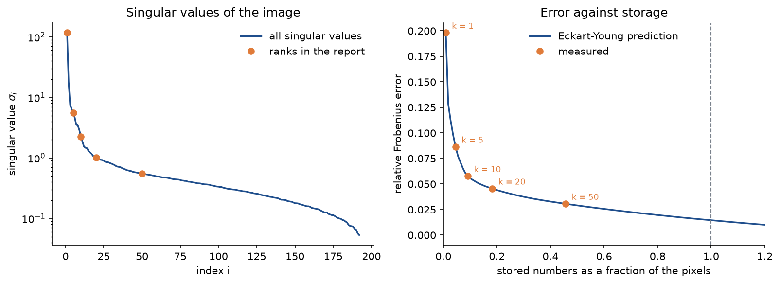
The spectrum explains the trade-off. The first singular value, 117.23, carries the average brightness and most of the energy, which is why the energy fraction is a poor guide to quality: 99 % of the energy is reached at rank 4, where the picture is still blurred. After about rank 20 the values settle onto a slowly falling floor made by the noise, which no low-rank approximation compresses, so extra triplets mostly store noise. The CC0 photograph from scikit-image shows the same shape with a slower fall: rank 50 stores 19.55 % of its numbers at 28.63 dB, 30 dB needs rank 65, 99 % of the energy needs rank 21 and the break-even rank is 255.

The notebook linear_algebra_for_ml.ipynb is a guided tour in the order of this page: vectors and maps, elimination, the worked example through trace_worked_example and again in bare NumPy, power iteration and the SVD, each pitfall, PCA on latent-factor data, image compression and the comparison with numpy.linalg. The tests in tests check the worked example value by value, the properties derived above and the agreement with NumPy, scikit-learn and SciPy, and run in a few seconds:

python -m pytest foundations/linear-algebra-for-ml

All data are synthetic, generated from fixed seeds by latent_factor_data, synthetic_image and the other generators in datasets.py, so nothing is downloaded. The optional photograph is the "camera" image bundled with scikit-image, released under CC0 by its photographer, Lav Varshney.

In practice

In production code these operations come from numpy.linalg and scipy.linalg, which call LAPACK. On a random 50 by 8 least-squares problem, examples/compare_with_libraries.py prints the largest difference between each from-scratch routine and its library equivalent, relative to the largest entry of the library result, after aligning the arbitrary signs of Q, eigenvectors and singular vectors:

• solve_linear_system against np.linalg.solve (LU with partial pivoting): 1.2 × 10⁻¹⁶.
• least_squares_normal and least_squares_qr against np.linalg.lstsq (SVD based): 5.6 × 10⁻¹⁶ and 7.4 × 10⁻¹⁶.
• qr_decomposition against np.linalg.qr (Householder): 4.7 × 10⁻¹⁶.
• symmetric_eigen against np.linalg.eigh: eigenvalues 4.7 × 10⁻¹⁶, eigenvectors 4.3 × 10⁻¹¹.
• svd_via_eigen against np.linalg.svd(a, full_matrices=False): singular values 2.8 × 10⁻¹⁶, left singular vectors 4.0 × 10⁻¹¹.
• solve_with_svd against np.linalg.pinv(a) @ b: 4.7 × 10⁻¹².
• condition_number against np.linalg.cond: 3.5 × 10⁻¹⁶; determinant against np.linalg.det: 7.8 × 10⁻¹⁶; rank against np.linalg.matrix_rank: equal.

The eigenvectors and singular vectors agree to about 10⁻¹¹ rather than 10⁻¹⁶. That is the effect of stopping power iteration at a residual of 10⁻¹² times the size of the matrix: an eigenvector's error is about the residual divided by the gap to the nearest other eigenvalue. The eigenvalues themselves converge twice as fast, so they agree to rounding error. The tests check each pair on random matrices, tall, wide and square. A comparison takes a few lines:

import numpy as np

from linear_algebra_for_ml import align_signs, svd_via_eigen

a = np.random.default_rng(0).normal(size=(50, 8))
ours = svd_via_eigen(a)
u, s, vt = np.linalg.svd(a, full_matrices=False)
print(np.max(np.abs(ours.s - s)), np.max(np.abs(ours.u - align_signs(ours.u, u))))

The same script runs PCA on 500 samples of 12 features driven by three hidden factors. It finds explained variance ratios of 0.5366, 0.4227 and 0.0325, followed by a flat floor of about 0.001 per component, so the first three components explain 0.9918 of the variance, and the reconstruction error with k components equals the sum of the discarded variances to within 1.4 × 10⁻¹⁴ for every k. Against sklearn.decomposition.PCA the explained variances agree to 5.3 × 10⁻¹⁶ and, after aligning signs, the components to 3.9 × 10⁻⁸ and the scores to 1.6 × 10⁻⁹; the larger differences come from the noise-floor components, whose eigenvalues are close together. The elimination null-space basis of the 3 by 4 matrix spans the same plane as scipy.linalg.null_space, to 9.9 × 10⁻¹⁶.

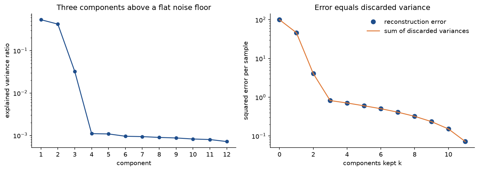
The left panel is the scree plot a practitioner reads to choose k: the elbow after the third component is the number of hidden factors. The right panel is Eckart-Young applied to PCA.

When to use which:

• Never solve least squares through np.linalg.inv(A.T @ A). Use np.linalg.lstsq or scipy.linalg.lstsq, or a QR factorization when the same A is reused with many right-hand sides. The normal equations are acceptable only when κ(A) is known to be small, for example after standardizing a handful of features, and their speed matters.
• For symmetric matrices use np.linalg.eigh, not eig. It is faster, returns real eigenvalues and orthonormal eigenvectors, and sorts eigenvalues in ascending order. eig is for general matrices, whose eigenvalues may be complex and whose eigenvectors need not be orthogonal.
• Use np.linalg.svd(a, full_matrices=False) for the thin SVD; the full version builds an m by m matrix U that is rarely needed. For the top few singular triplets of a large or sparse matrix, scipy.sparse.linalg.svds (Lanczos iterations) and randomized SVD (subspace iteration on a block of random vectors) build on the same repeated products with A and Aᵀ as power iteration.
• sklearn.decomposition.PCA centres the data (it does not scale it) and offers several solvers: a full SVD of the centred data, truncated SVDs by ARPACK or randomized subspace iteration, and, since version 1.5, an eigen-decomposition of the covariance matrix that is fast when there are many more samples than features and inherits the squared condition number. It reports explained_variance_ with the divisor m - 1, stores components_ as rows as PCAResult does, and fixes signs with its own convention.
• scipy.linalg.null_space and scipy.linalg.orth return orthonormal bases of the null space and column space from the SVD. They are more robust than the elimination-based null_space_basis, whose basis vectors are not orthogonal.
• Write these routines yourself to understand them, to reason about where accuracy is lost, and for the few algorithms that need a custom variant, such as power iteration on a matrix that is only available as a function computing A x. Low-rank factorizations also appear as models in their own right in recommender systems.

Pitfalls

• Solving the normal equations of an ill-conditioned problem. Their condition number is the square of that of A, so they lose twice as many digits as necessary. For a degree-9 polynomial fit in the monomial basis on 40 points in [0, 1], κ(A) = 3.5 × 10⁶ and κ(AᵀA) = 1.2 × 10¹³. The normal equations recover the coefficients with a relative error of 4.4 × 10⁻⁴, least_squares_qr with 4.3 × 10⁻¹¹ and np.linalg.lstsq with 5.1 × 10⁻¹¹. From degree 11 on, AᵀA is singular to working precision although A has full rank. Inverting AᵀA explicitly is worse still: on the degree-8 fit the inverse gives a relative error of 3.3 × 10⁻⁵ against 1.3 × 10⁻¹¹ for lstsq. examples/numerical_stability.py prints these numbers.

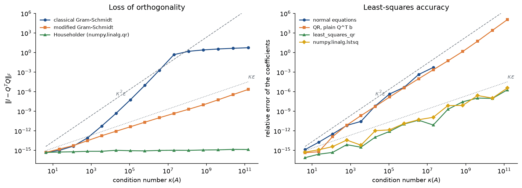
The two guide lines are the error levels κε and κ²ε. The squaring methods ride the upper line and the sound ones the lower.

• Classical Gram-Schmidt in floating point. Classical Gram-Schmidt loses orthogonality like κ²ε, modified Gram-Schmidt like κε, and Householder QR stays at ε. On the same polynomial fits the distance of QᵀQ from the identity at degree 9 is 2.0 × 10⁻³ for classical, 1.0 × 10⁻¹⁰ for modified and 1.0 × 10⁻¹⁵ for Householder, and at degree 11 the classical Q is no longer close to orthogonal at all (1.6). A related trap is computing Qᵀb as a plain product with a Gram-Schmidt Q that has lost orthogonality: in the figure that is no more accurate than the normal equations, while orthogonalizing b step by step, as least_squares_qr does, tracks lstsq.
• Computing the SVD through AᵀA. Squaring the singular values squares their spread. For singular values 1, 10⁻⁴ and 10⁻¹⁰, the eigenvalues of AᵀA include 10⁻²⁰, far below the rounding error of about 10⁻¹⁶ in its entries. The square roots of LAPACK's own eigvalsh(A.T @ A) give 6.5411 × 10⁻¹⁰ instead of 10⁻¹⁰, svd_via_eigen drops the value entirely, and np.linalg.svd on A recovers it. Use the from-scratch routine to learn and the library SVD for anything ill-conditioned; the same applies to PCA through the covariance matrix.
• Reading the wrong column after an eigen-decomposition. np.linalg.eigh returns eigenvalues in ascending order, so the direction of largest variance is the last column. Taking column 0 silently uses the direction of least variance, (0.4472, -0.8944) with variance 0.6667 for the worked example, instead of (0.8944, 0.4472) with variance 7.3333. The same slip happens when eigenvalues are sorted in descending order but the eigenvectors are not reordered with them; check that S v = λ v holds for the pair you use (examples/common_mistakes.py).
• Comparing eigenvectors or singular vectors without aligning signs. If v is an eigenvector, so is -v. eigh returns (-0.8944, -0.4472) for the worked example's top direction, and pca returns (0.8944, 0.4472). Tests and comparisons must align signs first, as align_signs does, and models that store components should fix a sign convention.
• PCA on uncentred data. Without centring, the first right singular vector points at the mean rather than along the spread. For points spread along the first axis around (0, 20) it is (0.0042, 1.0000), while the first principal component of the centred data is (1.0000, 0.0078). Fitting the mean and the components on all data before a train-test split is a separate mistake, a leak described in data leakage and pitfalls.
• Mixing the divisors m and m - 1. np.cov divides by m - 1 by default, np.var and np.std by m unless ddof=1. Principal directions and explained variance ratios do not depend on the choice, but reported variances differ by the factor m/(m - 1): for the first feature of the worked example np.var gives 4.5 and np.cov gives 6, a factor of 4/3.
• Treating a one-dimensional array as a column. NumPy vectors of shape (n,) have no orientation, so v.T does nothing. Subtracting an (n, 1) column from an (n,) vector broadcasts to an n by n matrix without any error: for the worked example, y - X @ w[:, None] has shape (4, 4) and a "sum of squared residuals" of 542.5455 instead of 0.3636.
• Testing singularity with the determinant or with exact zeros. The determinant measures volume, not conditioning. The determinant of 0.1 times the 30 by 30 identity is 10⁻³⁰ although the matrix is perfectly conditioned, and a 5 by 5 matrix of rank 3 has determinant 4.9 × 10⁻³³ rather than 0, with two singular values near 10⁻¹⁶. Rank needs a tolerance relative to the size of the entries or of σ1, as both rank and np.linalg.matrix_rank use.
• Confusing eigenvalues with singular values. They coincide only for symmetric positive semidefinite matrices. M has eigenvalues 2.5 and 1 but singular values 2.5583 and 0.9772, and its eigenvector lines through (2, 1) and (1, -1) meet at 71.57 degrees, not at a right angle. The largest stretch of a matrix is σ1, not the largest eigenvalue in magnitude.
• Expecting power iteration to converge without a gap. The error shrinks like the eigenvalue ratio to the power k. For the diagonal matrices in the convergence figure, ratios of 0.5, 0.9 and 0.99 need 39, 238 and 2257 iterations to reach the stopping tolerance. Eigenvalues 3 and -3 never separate: the iterate flips between (0.7071, -0.7071) and (0.7071, 0.7071). A start vector orthogonal to q1 would in exact arithmetic never find it; a random start avoids that.
• Covariance from the wrong product. With one example per row the covariance is XᵀX / (m - 1), an n by n matrix over features. XXᵀ is the m by m matrix of inner products between examples. It has the same nonzero eigenvalues (22 and 2 for the worked example, then two zeros), which is useful when m is smaller than n, but its eigenvectors are the left singular vectors, not the principal directions.

Further reading

• G. Strang, Introduction to Linear Algebra, sixth edition, Wellesley-Cambridge Press, 2023. The four fundamental subspaces, projections and the SVD, developed as on this page.
• S. Axler, Linear Algebra Done Right, fourth edition, Springer, 2024. Open access; a complete proof of the spectral theorem.
• L. N. Trefethen and D. Bau, Numerical Linear Algebra, SIAM, 1997. Gram-Schmidt and Householder QR, the conditioning of least squares and why the normal equations lose accuracy.
• G. H. Golub and C. F. Van Loan, Matrix Computations, fourth edition, Johns Hopkins University Press, 2013. The algorithms inside LAPACK.
• N. J. Higham, Accuracy and Stability of Numerical Algorithms, second edition, SIAM, 2002.
• M. P. Deisenroth, A. A. Faisal and C. S. Ong, Mathematics for Machine Learning, Cambridge University Press, 2020. Chapters 2 to 4 and 10 cover this page's material with machine learning in view.
• Å. Björck, "Solving linear least squares problems by Gram-Schmidt orthogonalization", BIT 7, 1-21, 1967. Why modified Gram-Schmidt with the right-hand side as an extra column is accurate.
• C. Eckart and G. Young, "The approximation of one matrix by another of lower rank", Psychometrika 1(3), 211-218, 1936.
• K. Pearson, "On lines and planes of closest fit to systems of points in space", Philosophical Magazine 2(11), 559-572, 1901. PCA as the best-fitting subspace.
• H. Hotelling, "Analysis of a complex of statistical variables into principal components", Journal of Educational Psychology 24, 417-441 and 498-520, 1933. PCA as variance maximization.
• R. von Mises and H. Pollaczek-Geiringer, "Praktische Verfahren der Gleichungsauflösung", Zeitschrift für Angewandte Mathematik und Mechanik 9, 58-77 and 152-164, 1929. The power method.
• N. Halko, P. G. Martinsson and J. A. Tropp, "Finding structure with randomness: probabilistic algorithms for constructing approximate matrix decompositions", SIAM Review 53(2), 217-288, 2011. Randomized SVD, the modern descendant of power iteration.