Search algorithms

Route planners, puzzle solvers, robot planners and game engines all face the same question: which sequence of actions leads from where we are to where we want to be, and which of those sequences is cheapest? Once a task is written down as states, actions, a transition model, a goal test and action costs, a handful of general algorithms answer it without knowing anything else about the domain. They differ only in the order in which they explore, and that order decides whether they find a solution at all, whether it is the cheapest one, and how much time and memory they spend. This page formulates search problems, explains tree search and graph search, derives the properties of breadth-first, depth-first, depth-limited, iterative deepening, uniform-cost, greedy best-first and A search, proves when A is optimal and shows what goes wrong when its heuristic overestimates. Every algorithm is run by hand on a small road network, a small maze and the 8-puzzle, implemented from scratch in Python, drawn as it explores larger mazes, measured with the effective branching factor and checked against networkx. Afterwards you will be able to formulate a new problem, pick the right algorithm, design a heuristic for it and prove that the heuristic keeps A* optimal. The page closes the Foundations part after Information theory and needs nothing from the earlier topics beyond comfortable Python.

To run the code in this topic, install the base group, and the data group for the comparison with networkx.

Intuition

Imagine standing at the start with a map that reveals a place only when you visit it. From the start you can see the places one action away. Each of them, once visited, reveals the places one action further, and so on. At any moment the places you know about split into two groups: those you have already visited, the explored set, and those you have seen but not yet visited, the frontier. The frontier is the boundary between the explored region and the unknown, and every search algorithm on this page is the same loop around it.

The loop never changes. What changes is the strategy, the rule that decides which frontier node leaves next, and the data structure that implements it.

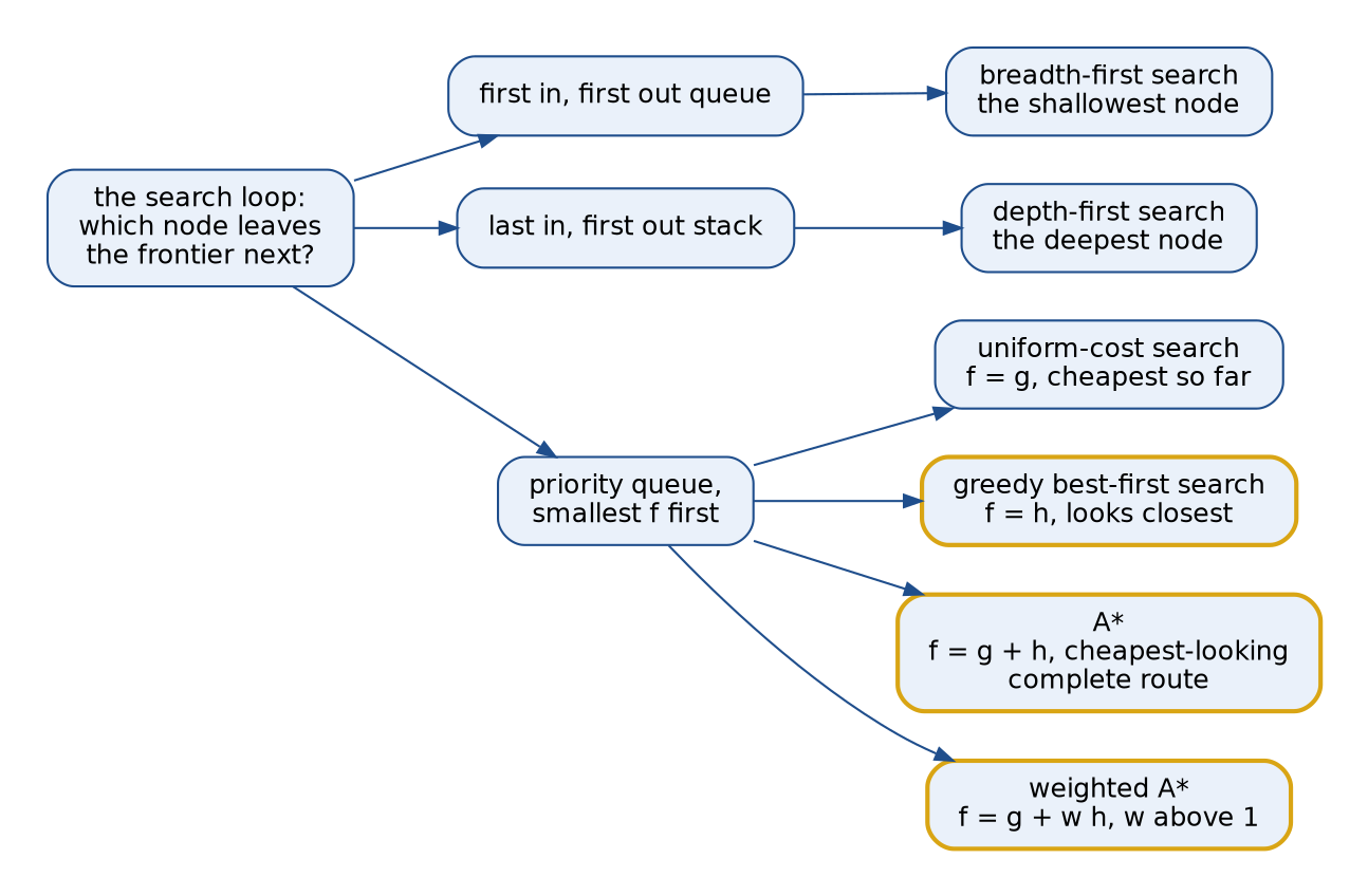
The diagram sorts the algorithms by their frontier:

• Breadth-first search uses a first-in first-out queue and removes the shallowest node, the one with the fewest actions from the start.
• Depth-first search uses a last-in first-out stack and removes the deepest node, the newest child.
• Uniform-cost search uses a priority queue on the path cost g and removes the node reached most cheaply so far.
• Greedy best-first search uses a priority queue on the heuristic h and removes the node that looks closest to the goal.
• A* uses a priority queue on g + h and removes the node on the cheapest-looking complete route.

Breadth-first and depth-first search are uninformed: they use nothing but the problem definition. Greedy best-first search and A are informed: a heuristic estimates the remaining cost from each state, and a good estimate lets the search head for the goal instead of spreading out evenly. Greedy search trusts the estimate completely and can be lured down an expensive route. A balances the cost already paid against the estimated cost still to come, and as long as the estimate never exceeds the true remaining cost it still returns the cheapest route, usually after exploring far less than uniform-cost search.

How it works

Notation

The symbols used on this page:

• The initial state is s0. ACTIONS(s) is the finite set of actions available in state s, RESULT(s, a) is the state that action a leads to, the transition model, and c(s, a, s′) is that action's cost, never negative. The goal test may accept one state or many.
• A node n is a state together with the path that reached it. Its path cost g(n) is the sum of the action costs along that path, and g*(s) is the cost of the cheapest path from s0 to the state s.
• A heuristic h(n) estimates the cost from the state of n to a goal, and h*(n) is the true cost of the cheapest such path.
• The evaluation function f(n) orders the frontier, C* is the cost of an optimal solution, and ε is a positive lower bound on every action cost.
• The branching factor b is the largest number of actions in any state, d is the number of actions of the shallowest solution, m is the largest depth of any path, possibly infinite, and l is the depth limit of depth-limited search.
• N is the number of nodes a search generates, b its effective branching factor, and w the weight of weighted A.

The formula images write the starred quantities with a superscript star and indices as subscripts. In the text they appear as g, h, C and b, and powers are written as superscripts, so bᵈ is b to the power d.

Formulating a search problem

A search problem has five components:

1. The initial state s0.
2. The actions: for every state s, the finite set ACTIONS(s).
3. The transition model RESULT(s, a), the state an action leads to.
4. The goal test, which may accept one state or many.
5. The action cost function c(s, a, s′).

The states and actions form a directed graph with an edge from s to RESULT(s, a) for every action, weighted by its cost. A solution is a sequence of actions whose transitions lead from s0 to a goal state. A node n reached by the actions a1 to ak through the states s0 to sk has the path cost

and an optimal solution has the smallest cost C* among all solutions. Three examples run through this page:

• Route finding on a road network. A state is a place, an action drives along one road, the transition model gives the place at its other end, the goal test checks for the destination, and the cost is the road's length or driving time.
• A grid maze. A state is a cell (r, c), the actions move to a free neighbouring cell, in four directions or eight with diagonals, and a move costs 1, √2 for a diagonal, or more on difficult terrain.
• The 8-puzzle. A state is an arrangement of tiles 1 to 8 and one blank on a 3 by 3 board, an action moves the blank up, down, left or right by swapping it with the neighbouring tile, and every action costs 1.

Formulation is abstraction: a route planner ignores the radio and the weather, a puzzle state ignores how the tiles are held. The abstraction is valid when every abstract solution can be carried out in the real world, and useful when the abstract actions are easier to search over than the real ones.

A node is not a state. A node records a state, its parent node, the action that produced it, its path cost g and its depth. Many nodes can hold the same state, reached by different paths, and following parent links from a goal node back to the root recovers the solution.

Tree search, graph search and the explored set

Tree search runs the loop with no memory of the states it has seen. Every path is a separate branch of a search tree, so a state reachable along many paths is expanded many times, and a state space with cycles produces an infinite tree.

The diagram unrolls a four-state cycle. Two levels down, the tree already holds A three times and D twice, and every further level doubles the waste. On an open 4-connected grid the growth is easy to count: tree search generates one path per sequence of k moves, while far fewer distinct cells lie within k moves of the start.

At k = 10 that is 1,048,576 paths for 221 cells.

Graph search adds a table of reached states, the union of the explored set and the frontier. A child whose state is already in the table is discarded, unless the search orders its frontier by path cost and the child reaches the state more cheaply, in which case the cheaper node replaces the old one. Graph search therefore expands each state at most once, or a few times when cheaper paths arrive late, and its memory grows with the number of distinct states reached rather than with the number of paths.

The frontier separates the explored states from the rest: every path from s0 to a state that has not been explored passes through a frontier state. This holds initially, when the frontier holds s0 and nothing is explored, and every expansion preserves it, because the expanded state moves to the explored set while all its successors join the frontier or are already reached. The optimality proofs below rest on this separation.

Where the goal test happens matters. Breadth-first search may test each child as soon as it is generated, because the first node generated for any state lies on a path with the fewest actions. Uniform-cost search and A* must test a node when it is removed from the frontier: the first path to reach the goal is not necessarily the cheapest, as the worked example shows.

Breadth-first search

Breadth-first search expands the shallowest frontier node first, which a first-in first-out queue does automatically. All nodes at depth k are expanded before any node at depth k + 1, so the first goal generated is at the smallest depth d.

• It is complete when b is finite: the level at depth d holds finitely many nodes and is reached after finitely many expansions.
• It is optimal when every action has the same cost, since then fewest actions means cheapest. With different costs it is not: in the worked example it finds a route costing 17 where 11 is possible.
• With the goal test on generation, the number of nodes it generates in the worst case is

and every node of the last level sits on the frontier at once, so time and space are both O(bᵈ). Memory, not time, is usually what stops breadth-first search. Testing on expansion instead generates part of the next level as well, up to b to the power d + 1 nodes.

Depth-first search

Depth-first search expands the deepest frontier node first, with a last-in first-out stack. It follows one line of actions until it reaches a goal or a dead end and then backs up to the most recent state with an untried action.

• Tree search with a check that rejects a state already on the current path needs to store only the current path and the untried siblings along it, O(bm) nodes. This small memory is the reason to use it. It is complete only in finite state spaces, where the number of paths without repeated states is finite; without the cycle check it can walk back and forth between two states forever.
• Graph search is complete in finite state spaces but stores every state it has explored, which removes the memory advantage.
• It is not optimal: it returns the first solution along its line, however long. Its time is O(bᵐ), terrible when m is much larger than d, and the answer depends on the order in which the actions are listed.

Depth-limited and iterative deepening search

Depth-limited search is depth-first tree search that treats nodes at depth l as if they had no successors. It always terminates, in time O(bˡ) and space O(bl), but it has two ways to fail that must be kept apart: cutoff, when some node was cut off at the limit so a deeper solution might exist, and failure, when no node was cut off, so every path from the start was followed to its end without finding a goal.

Iterative deepening runs depth-limited search with the limits 0, 1, 2 and so on until a run does not end in cutoff. The first successful limit is d, so the solution has the fewest actions, as with breadth-first search, while the memory is that of depth-first search, O(bd). The upper levels are regenerated in every iteration, but in a tree they hold few nodes. A node at depth i is generated once in each of the iterations with limits i to d, that is d + 1 - i times, so the totals are

Factoring out bᵈ and substituting j = d - i turns their ratio into a weighted mean of j + 1, with weights proportional to b to the power -j, which grows with d towards a simple limit:

The limit uses two geometric series in x = 1/b: the sum of (j + 1)xʲ is (1 - x)⁻² and the sum of xʲ is (1 - x)⁻¹. For b = 4 and d = 6, breadth-first search generates 5460 nodes and iterative deepening 7272, a ratio of 1.3319 against the limit 1.3333. The repetition is cheap when the tree is bushy and expensive when b is close to 1, as in a maze of corridors.

Uniform-cost search

Uniform-cost search orders the frontier by path cost, f(n) = g(n), and tests for the goal when a node is removed. It is Dijkstra's algorithm run on the state graph from the initial state, generating states lazily and stopping at the first goal removed from the queue.

Claim: if every action cost is non-negative, then whenever a node for a state s is removed from the frontier, its path cost equals g(s). Proof sketch: suppose a node n for s is removed with a path cost above g(s). Take an optimal path to s. By the separation property it contains a frontier state; let s′ be the first state on the path that has not been explored. Its predecessor on the path was explored with its optimal cost, by induction over the order of removals, so the frontier holds a node n′ for s′ with

where the middle step uses that costs are non-negative. The priority queue would have removed n′ first, a contradiction.

So the first goal removed is reached by an optimal path. The proof uses non-negative costs in one place, the inequality g(s′) ≤ g(s); with negative costs the claim fails and Bellman-Ford is needed. Completeness needs every action cost to be at least some ε > 0, since a cycle of zero-cost actions can keep the search busy forever. Every node with a path cost below C is expanded, and such a node has a depth of at most C/ε rounded down, so time and space are

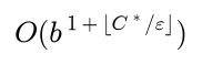
which can be far more than bᵈ when there are many cheap actions.

Greedy best-first search

Greedy best-first search orders the frontier by the heuristic alone, f(n) = h(n). It ignores the cost already paid, so it is not optimal: in the worked example it reaches the goal through a place that looks close but is joined to the goal by an expensive road. Tree search can oscillate between two states that each look closer than the other's neighbours; graph search is complete in finite state spaces. The worst case is O(bᵐ) time and space, but with a good heuristic it often expands little more than the nodes on the path it returns.

A* search

The three best-first searches differ only in their evaluation function:

For A*, f(n) estimates the cost of the cheapest solution through n: the cost of the path so far plus the estimated cost to finish. With h = 0 it is uniform-cost search. Two properties of h govern its behaviour. A heuristic is admissible if it never overestimates, so in particular h = 0 at every goal:

A heuristic is consistent if it is zero at every goal and obeys a triangle inequality along every action, where n′ is the child of n that the action produces:

Consistency compares the estimate before an action with the action's cost plus the estimate after it: an estimate cannot fall by more than the price of the step.

Lemma 1: a consistent heuristic is admissible. Let sk, sk-1 down to s0 be the states of an optimal path from the state of n to a goal s0, with step costs ck down to c1. Applying consistency k times and using h(s0) = 0 gives

The converse is false; the inconsistent example under Pitfalls is admissible.

Lemma 2: with a consistent heuristic, f never decreases along a path. For a child n′ of n:

Theorem 1, for an admissible heuristic: A as tree search, or as graph search that reopens a closed state when a cheaper path to it is found, returns an optimal solution. Proof sketch: suppose A is about to return a goal node G2 with a path cost above C*. Fix an optimal solution path. At every moment some node of it sits on the frontier with its optimal path cost: initially the root, and whenever that node is expanded, its successor on the path is added with its optimal cost or is already held at that cost; reopening guarantees that a closed state does not block this. Call that frontier node n. Then

so n has a smaller priority than G2 and is removed first. Repeating the argument, every node of the optimal path is removed before G2, including its goal, which ends the search with cost C*, a contradiction.

Theorem 2, for a consistent heuristic: A as graph search that never reopens closed states returns an optimal solution, and the first time a state is removed from the frontier its path cost is already optimal. By Lemma 2 the priorities of the removed nodes never decrease. Repeat the uniform-cost argument with f in place of g: if a node n for a state s were removed with a path cost above g(s), the first unexplored state s′ on an optimal path to s would be on the frontier in a node n′ with

where the first inequality applies consistency along the optimal path from s′ to s. So n′ would have been removed first.

Consequences:

• A expands every node with f(n) < C and no node with f(n) > C; nodes with f(n) = C depend on how ties are broken.

• With a consistent heuristic the expanded region grows in contours of increasing f, stretched towards the goal by h; with h = 0 they are rings of constant g around the start.
• Among algorithms that extend paths from the start and use the same admissible heuristic, none is guaranteed to expand fewer nodes, apart from ties (Dechter and Pearl, 1985). A is optimally efficient in this sense, which is about node counts, not memory: A keeps every generated node, and memory is usually its limit.
• With an admissible but inconsistent heuristic, a graph search that never reopens closed states can return a suboptimal solution, as the Pitfalls section shows. Reopening restores optimality at the price of re-expansions, exponentially many in contrived worst cases (Martelli, 1977).

Overestimating heuristics and weighted A*

Theorem 1 breaks at the inequality h(n) ≤ h(n): a node on the optimal path can look worse than a suboptimal goal, and A returns that goal. The worked example below overestimates at a single place and A returns a route costing 12 instead of 11. The damage can be bounded when the overestimate is controlled. Weighted A multiplies an admissible heuristic by a weight:

When it removes a goal G, the frontier node n on the optimal path from Theorem 1 satisfies

so the returned cost is at most w times the optimum. The argument uses reopening; the same bound holds without reopening when h is consistent (Likhachev, Gordon and Thrun, 2003). A larger w makes the search greedier and usually much faster. examples/grid_heuristics.py measures this on ten solvable 60 by 80 grids with a quarter of the cells blocked, diagonal moves and the octile distance described below:

• w = 1: 1399.0 expansions on average, every path optimal.
• w = 1.25: 300.1 expansions, paths 3.63 % longer on average and 6.51 % longer on the worst grid.
• w = 1.5: 216.2 expansions, 5.02 % longer on average and 11.16 % on the worst grid.
• w = 2: 141.5 expansions, 4.95 % longer on average and 8.43 % on the worst grid.
• w = 3 and w = 5: 133.3 and 134.2 expansions, 5.42 % and 8.11 % longer on average, 9.17 % and 15.80 % on the worst grid.

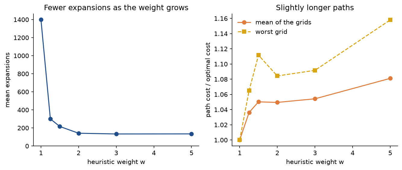
A weight of 1.25 already cuts the expansions by 79 % for paths 3.6 % longer on average, far inside the guaranteed bound of 25 %. Beyond w = 2 the search is essentially greedy and the expansions stop falling.

Designing heuristics from relaxed problems

A relaxed problem drops some of the restrictions on the actions, so it has more edges than the original state graph. Every original path is still a path in the relaxed graph, so the cost of an optimal relaxed solution is at most the original cost:

The relaxed cost is therefore admissible. It is also consistent, because it is a shortest-path distance in the relaxed graph, and shortest-path distances obey the triangle inequality along every original edge, which is also a relaxed edge.

Grid mazes. Relax by deleting the walls; the cost to the goal in an empty grid becomes a closed formula in the row offset Δr and the column offset Δc between a cell and the goal cell (rG, cG):

• With four moves of cost 1, an empty grid needs exactly Δr + Δc moves: the Manhattan distance.
• With diagonal moves of cost √2 as well, the cheapest empty-grid route makes as many diagonal moves as the smaller offset allows and finishes with straight moves, which gives the octile distance:

• The Euclidean distance relaxes further, to motion in any direction in the plane. It is admissible on both kinds of grid but smaller than the octile distance on 8-connected grids and than the Manhattan distance on 4-connected ones, so it guides less. The Chebyshev distance is exact for diagonal moves of cost 1 and admissible, but weaker still, when diagonals cost √2.
• The Manhattan distance on an 8-connected grid is not a relaxation. It overestimates every diagonal: three diagonal moves cost 3√2 = 4.2426, but Δr + Δc = 6.
• When cells cost different amounts to enter, scale the distance by the cheapest cost per move, or the estimate overestimates on cheap terrain.

examples/grid_heuristics.py runs A* with each of these on a 40 by 60 grid with 25 % of the cells blocked and diagonal moves of cost √2 that may not cut a blocked corner. The optimal path costs 83.9411:

• The zero heuristic, which makes A* uniform-cost search, expands 1787 cells.
• The Chebyshev distance expands 1092, the Euclidean distance 906 and the octile distance 713, all admissible and consistent and all returning cost 83.9411.
• The Manhattan distance overestimates at 1525 of the 1788 reachable cells, is neither admissible nor consistent, expands only 93 cells and returns a path of cost 85.1127, 1.4 % too long.

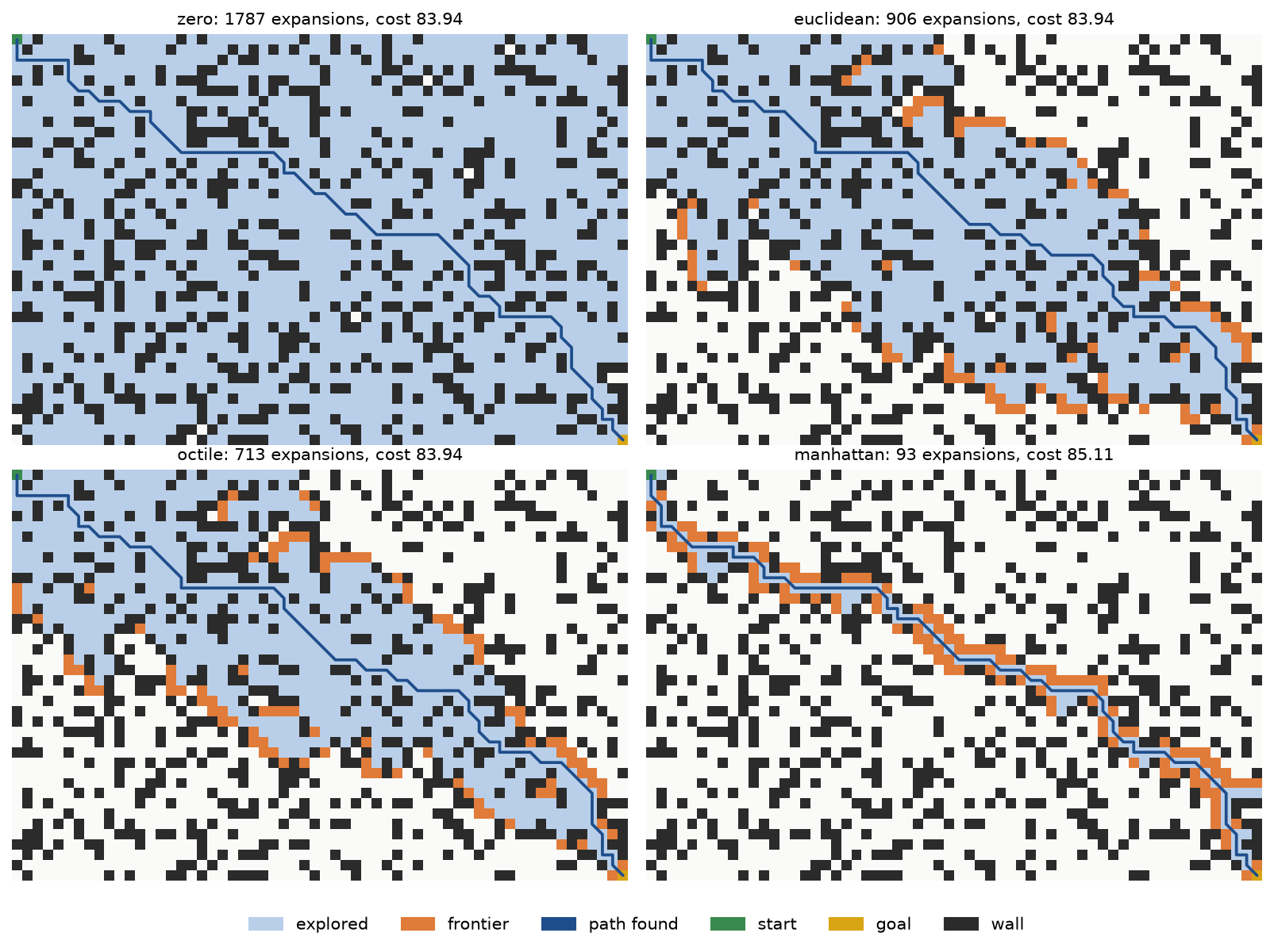
Each admissible heuristic is larger than the one before it and expands fewer cells, and the exact empty-grid cost, the octile distance, expands 60 % fewer than uniform-cost search. The thin strip of the Manhattan run is what an overestimate buys: speed at the price of the guarantee.

The 8-puzzle. A tile can move from square A to square B if A and B are adjacent and B is blank. Dropping both conditions lets a tile jump anywhere in one move, and the relaxed cost is the number of misplaced tiles, h1. Dropping only the blank condition lets tiles slide through each other, and the relaxed cost is the sum of the tiles' Manhattan distances to their home squares, h2. Every misplaced tile is at least one square from home, so h2 dominates h1:

Domination pays off. With consistent heuristics, A expands every node with g(n) + h(n) < C. If h2 ≥ h1 everywhere, every node satisfying the condition for h2 satisfies it for h1 too, so A with h2 never expands a node that A* with h1 would skip, apart from ties. Given several admissible heuristics, their maximum is admissible and dominates each of them, and it is consistent if each of them is:

The maximum costs one evaluation of each heuristic per node, which is usually far cheaper than the expansions it saves.

The effective branching factor

Node counts grow exponentially with depth, so they are hard to compare across problems. The effective branching factor b* summarises a search that generated N nodes to find a solution at depth d: it is the branching factor of a uniform tree of depth d that contains N + 1 nodes, the extra one counting the root.

The right-hand side increases with b, from d + 1 at b = 1, so the equation has exactly one solution for N ≥ d, found by bisection. A perfect heuristic that generates only the path has b = 1. For a given heuristic b tends to be fairly stable across depths, so measuring it on small instances predicts the cost of large ones. Here N counts every child added to the frontier, including a state added again with a cheaper path, but not the root.

examples/eight_puzzle.py measures it on the 8-puzzle. A breadth-first sweep backwards from the goal labels every one of the 9!/2 = 181,440 solvable boards with its optimal solution length; the two hardest boards need 31 moves. For each even depth up to 24, 50 boards with exactly that optimal length are drawn at random (all of them at depths 2 and 4, which have only 4 and 16 boards, and 39 at depth 6), and each search counts the nodes it generates. Breadth-first search runs up to depth 18 and iterative deepening up to depth 14, beyond which they become slow. The mean counts, with the b* of each mean in parentheses:

• Depth 6: iterative deepening 169.5 (2.12), breadth-first 78.9 (1.82), A with misplaced tiles 15.1 (1.27), A with the Manhattan distance 12.7 (1.22).
• Depth 12: iterative deepening 5161.9 (1.92), breadth-first 1587.3 (1.72), misplaced tiles 136.3 (1.35), Manhattan 44.1 (1.19).
• Depth 14: iterative deepening 15616.2 (1.89), breadth-first 4120.5 (1.70), misplaced tiles 295.5 (1.37), Manhattan 72.7 (1.20).
• Depth 18: breadth-first 23275.0 (1.66), misplaced tiles 1659.0 (1.41), Manhattan 251.2 (1.24).
• Depth 24: misplaced tiles 19932.6 (1.44), Manhattan 1484.9 (1.27).

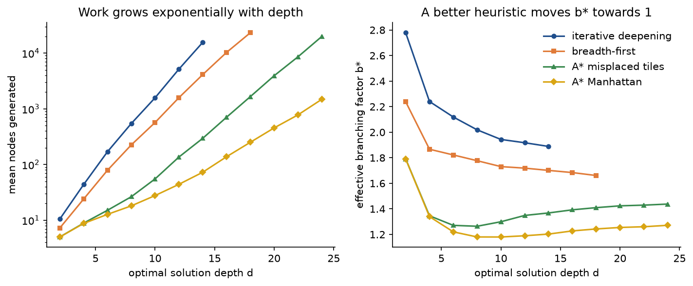
Every count rises as a straight line on the logarithmic axis, which is exponential growth, and the slope is set by b. At depth 24 the Manhattan heuristic generates 13 times fewer nodes than misplaced tiles, and its b stays between 1.18 and 1.27 from depth 6 on. Iterative deepening generates 3.8 times as many nodes as breadth-first search at depth 14, much more than the overhead b/(b - 1) of the earlier section: it is a tree search, and the 8-puzzle is full of short cycles whose repeated states breadth-first graph search discards. The example prints the full measurement for every even depth.

Properties of the algorithms

With b finite, every action costing at least ε > 0 and the heuristics as stated:

• Breadth-first search: complete, optimal when all actions cost the same, time and space O(bᵈ).
• Uniform-cost search: complete and optimal, time and space of order b to the power 1 + C*/ε rounded down, as shown above.
• Depth-first tree search with a cycle check: complete only in finite spaces, not optimal, time O(bᵐ), space O(bm).
• Depth-first graph search: complete only in finite spaces, not optimal, time O(bᵐ) but at most the number of states, space the number of states.
• Depth-limited search: complete only when l ≥ d, not optimal, time O(bˡ), space O(bl).
• Iterative deepening: complete, optimal when all actions cost the same, time O(bᵈ), space O(bd).
• Greedy best-first graph search: complete only in finite spaces, not optimal, time and space O(bᵐ).
• A: complete, and optimal with an admissible heuristic when closed states can be reopened or with a consistent heuristic otherwise. It expands every node with f < C, exponentially many in d in the worst case, and keeps every generated node in memory.

Worked example

The road network

Seven places joined by two-way roads, with driving times as costs. The task is to get from S to G. Place C lies just across a river from G, so it looks close, but the only road from C to G goes round by a distant bridge and costs 10.

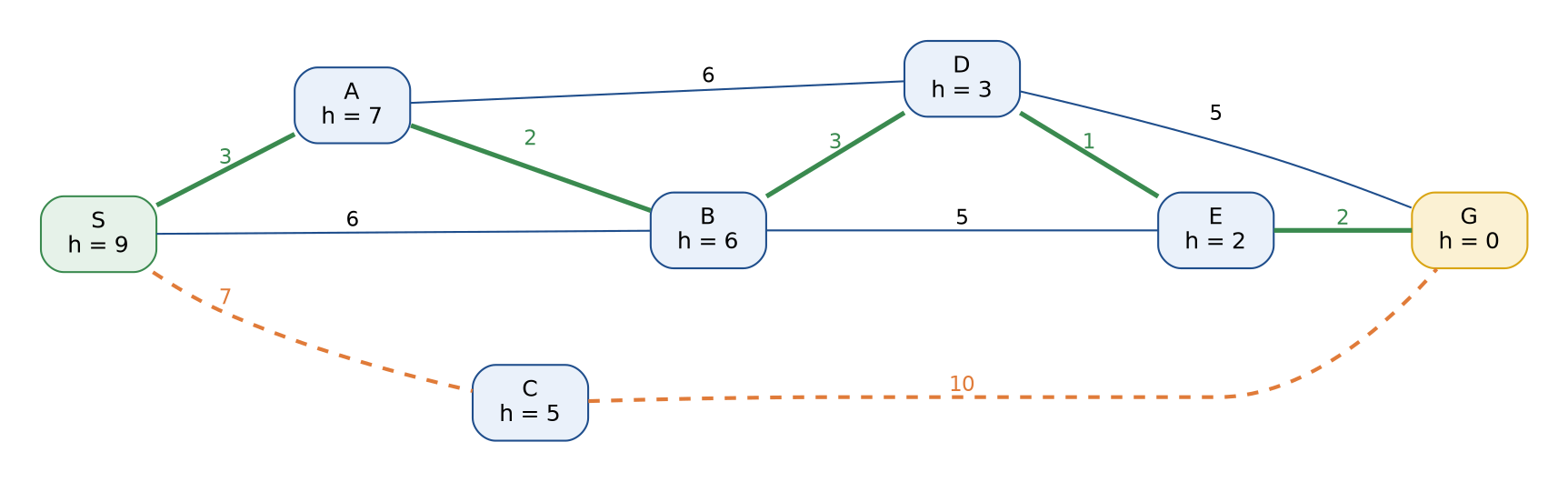
The formulation: states are the seven places, s0 is S, ACTIONS(s) lists the roads leaving s in alphabetical order of their far ends, RESULT(s, a) is the place at the far end of road a, the goal test accepts only G, and the cost is the road's driving time. The heuristic h is an estimate of the remaining driving time, and h* is the true remaining cost, computed by running Dijkstra's algorithm backwards from G:

• S: h = 9, h = 11. A: h = 7, h = 8. B: h = 6, h = 6. C: h = 5, h = 10.
• D: h = 3, h = 3. E: h = 2, h = 2. G: h = 0, h* = 0.

h never exceeds h*, so it is admissible. It is also consistent: across every road the estimate changes by at most the road's cost. For example, h(A) - h(B) = 1 ≤ 2 and h(C) - h(G) = 5 ≤ 10, and equality holds on the roads B to D, D to E and E to G. The optimal route is S, A, B, D, E, G with cost 3 + 2 + 3 + 1 + 2 = 11, drawn in green; the dashed orange route S, C, G uses only two roads but costs 7 + 10 = 17.

Breadth-first search

The goal test happens on generation and children are added in alphabetical order. The frontier is shown after each expansion; states already reached are not added again.

1. Expand S, add A, B and C. Frontier A, B, C.
2. Expand A, add D; B and S are already reached. Frontier B, C, D.
3. Expand B, add E. Frontier C, D, E.
4. Expand C, add G, which passes the goal test.

Breadth-first search returns S, C, G after 4 expansions and 6 generated nodes. It has the fewest roads, two, and costs 7 + 10 = 17.

Uniform-cost search by hand

Each frontier entry is shown as the state and its path cost g. When a child reaches a state already on the frontier more cheaply, it replaces the old entry.

1. Expand S at g = 0. Frontier A 3, B 6, C 7.
2. Expand A at g = 3. B is reached for 3 + 2 = 5 < 6. Frontier B 5, C 7, D 9.
3. Expand B at g = 5. D is reached for 5 + 3 = 8 < 9. Frontier C 7, D 8, E 10.
4. Expand C at g = 7. Frontier D 8, E 10, G 17.
5. Expand D at g = 8. E is reached for 8 + 1 = 9 < 10 and G for 8 + 5 = 13 < 17. Frontier E 9, G 13.
6. Expand E at g = 9. G is reached for 9 + 2 = 11 < 13. Frontier G 11.
7. Remove G at g = 11: the goal.

The goal enters the frontier at step 4 with the expensive path through C, cost 17, and its entry improves twice before it is removed at cost 11. Uniform-cost search returns S, A, B, D, E, G with cost 11 after 6 expansions and 11 generated nodes. A goal test on generation would have stopped at step 4 with cost 17.

Greedy best-first search

The frontier is ordered by h alone:

1. Expand S at h = 9. Frontier C 5, B 6, A 7.
2. Expand C at h = 5. Frontier G 0, B 6, A 7.
3. Remove G: the goal.

Two expansions and the route S, C, G with cost 17: the estimate 5 at C made the river crossing look short.

A* by hand

The frontier is ordered by f = g + h. Entries with equal f are listed in the order they leave the frontier: smaller h first, then first in, first out. At step 1, A gets f = 3 + 7 = 10, B gets 6 + 6 = 12 and C gets 7 + 5 = 12.

1. Expand S at g = 0, f = 9. Frontier A 10, C 12, B 12.
2. Expand A at g = 3, f = 10. B is reached for g = 5, f = 5 + 6 = 11. Frontier B 11, D 12, C 12.
3. Expand B at g = 5, f = 11. D is reached for g = 8, f = 8 + 3 = 11. Frontier D 11, E 12, C 12.
4. Expand D at g = 8, f = 11. E is reached for g = 9, f = 9 + 2 = 11. Frontier E 11, C 12, G 13.
5. Expand E at g = 9, f = 11. G is reached for g = 11, f = 11 + 0 = 11. Frontier G 11, C 12.
6. Remove G at g = 11: the goal.

A returns the optimal route S, A, B, D, E, G, cost 11, after 5 expansions and 10 generated nodes. The removed priorities 9, 10, 11, 11, 11 and 11 never decrease, as Lemma 2 promises for a consistent heuristic, and every node on the optimal route has f ≤ C = 11. C, with f = 12 > C, is never expanded; that is the one expansion A saves over uniform-cost search here.

An overestimating heuristic

Change a single entry to h(D) = 8, five more than the true remaining cost of 3, and run A* again:

1. Expand S at g = 0, f = 9. Frontier A 10, C 12, B 12.
2. Expand A at g = 3, f = 10. Frontier B 11, C 12, D 17.
3. Expand B at g = 5, f = 11. Frontier E 12, C 12, D 16.
4. Expand E at g = 10, f = 12. Frontier G 12, C 12, D 16.
5. Remove G at g = 12: the goal.

D, which lies on the optimal route, now has f = 8 + 8 = 16, larger than the cost of the route through E. A returns S, A, B, E, G with cost 3 + 2 + 5 + 2 = 12 after 4 expansions: one fewer than before, and one unit worse. In Theorem 1, the frontier node D on the optimal path has f(D) = 16 > C = 11, so the inequality the proof needs is exactly what fails.

Depth-first and iterative deepening search on the same roads

Depth-first graph search, taking the alphabetically first road each time, expands S, A, B, D and E and returns the route S, A, B, D, E, G. It happens to be the cheapest, but it uses five roads where two suffice; with the roads listed in reverse order the same algorithm goes straight to C and returns S, C, G at cost 17. Iterative deepening expands nothing with limit 0, since the root sits at the limit, S with limit 1, and S, A, B and C with limit 2, where it finds G below C: 0, 1 and 4 expansions, and the same answer as breadth-first search.

A small maze

Moves go up, right, down or left, tried in that order, and each costs 1. The start is the top-left cell and the goal G the bottom-left one, but a wall forces every route round a detour.

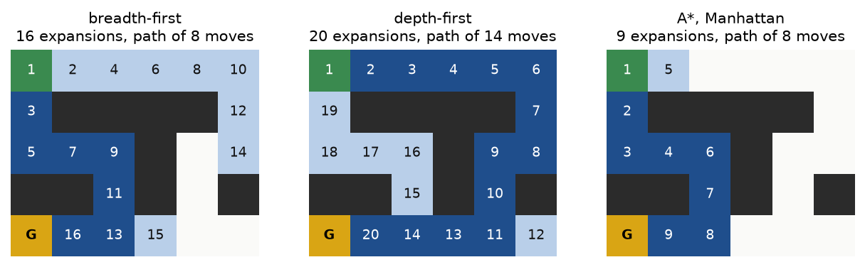
The numbers give the order of expansion, and unnumbered open cells were never expanded.

• Breadth-first search fans out in rings of equal distance and generates G while expanding cell 16, the cell to its right: 16 expansions and a path of 8 moves, the shortest.
• Depth-first search runs along the top corridor, down the right side, into a dead end at the bottom right, back along the bottom row, up through the middle and round the left side before it expands the cell next to G: 20 expansions and a path of 14 moves.
• A with the Manhattan distance, h(r, c) = |r - 4| + |c|, goes down first. S has f = 0 + 4 = 4, and so do the two cells below it. At cell 3, (2, 0), the wall below forces a detour: (2, 1) has f = 3 + 3 = 6, tied with (0, 1) at f = 1 + 5 = 6. The smaller h goes first, and (0, 1) follows as expansion 5 because its f = 6 is still below C = 8. From then on every cell on the way down has f = 8: 9 expansions and a path of 8 moves.
• Greedy best-first search follows the same route without expanding (0, 1): 8 expansions. Uniform-cost search, which tests the goal on removal, needs 18.
• Iterative deepening expands 0, 1, 3, 5, 7, 9, 11, 13 and 16 cells with the limits 0 to 8, 65 in total. The maze is a corridor with a branching factor close to 1, the case in which repeating the upper levels is expensive: the last iteration alone needs 16.
• Breadth-first tree search, without the table of reached states, still returns a path of 8 moves but expands 244 nodes and generates 489, because it walks back and forth through the same cells.

The 8-puzzle heuristics

The goal arrangement has the rows 1 2 3, 4 5 6 and 7 8 blank. Take the board with the rows 4 2 1, 7 blank 3 and 5 8 6.

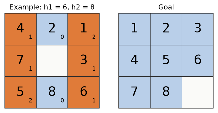
Six tiles are misplaced, 4, 1, 7, 3, 5 and 6, while 2 and 8 are home, so h1 = 6. Their Manhattan distances to their home squares are 1 for tile 4, 0 for tile 2, 2 for tile 1, 1 for tile 7, 1 for tile 3, 2 for tile 5, 0 for tile 8 and 1 for tile 6, so h2 = 8. The optimal solution has 12 moves, so h1 = 6 ≤ h2 = 8 ≤ h* = 12.

A generates 136 nodes with h1 and 36 with h2; breadth-first search generates 1588. For A with h2, the effective branching factor solves 1 + b + ... + b¹² = 37. Trying two values by hand brackets it:

So b lies a little above 1.16, and bisection gives b = 1.1608. The same equation gives b = 1.3485 for h1 and 1.7189 for breadth-first search. A search that generated only the path would have b = 1.

Every number in this section is printed by examples/road_network.py, examples/small_maze.py and examples/eight_puzzle.py, and asserted by the tests, from the traces in tests/test_best_first.py to the expansion orders in tests/test_breadth_first.py and the 8-puzzle counts in tests/test_puzzle.py and tests/test_complexity.py.

The code

The package search_algorithms uses the standard library and NumPy, one module per idea. networkx is imported only inside the functions of comparisons.py, and Matplotlib only by the two plotting modules.

• problems.py holds the SearchProblem protocol with initial, actions, result, action_cost and is_goal, the type names shared by the other modules, and zero_heuristic.
• nodes.py holds Node, which records a state, its parent, the action, the path cost and the depth, and expand, which yields the children.
• results.py holds SearchResult with its status (solved, failure, cutoff or budget), the goal node, the counts of expanded and generated nodes, the largest frontier, the expansion order, snapshots and an optional trace.
• breadth_first.py, depth_first.py and depth_limited.py hold the uninformed searches: breadth_first_search as tree or graph search with the goal test on generation or expansion, depth_first_search as graph search or tree search with or without a cycle check, depth_limited_search and iterative_deepening_search.
• best_first.py holds best_first_search(problem, evaluation, heuristic) and the three wrappers uniform_cost_search, greedy_best_first_search and astar_search, with options for reopening closed states, the goal test on generation, tie-breaking, the cost tolerance and the weight of weighted A*.
• graphs.py holds GraphProblem, the road network of the worked example, the network of the reopening pitfall and random_graph.
• grids.py holds GridMaze with 4- or 8-connected moves, no corner cutting and digits for terrain costs; mazes.py carves mazes with generate_maze and scatters obstacles with random_grid.
• heuristics.py holds the grid distances manhattan, euclidean, octile and chebyshev, table_heuristic for explicit tables and max_heuristic.
• puzzle.py holds EightPuzzle, misplaced_tiles, tile_manhattan, the fast puzzle_heuristic, the solvability test and puzzle_distances, which labels every board with its optimal solution length.
• analysis.py holds state_space, costs_to_goal, admissibility_violations, consistency_violations and path_cost, which check a heuristic against the truth on any problem small enough to sweep.
• complexity.py holds effective_branching_factor, tree_size and the node counts of breadth-first search and iterative deepening on uniform trees.
• tracing.py prints traces, routes and expansion orders; maze_plots.py draws snapshots, expansion orders and puzzle boards; plotting.py draws the charts and saves figures reproducibly.
• experiments.py holds the measurements behind the figures: solve_maze, heuristic_runs, weighted_astar_sweep and puzzle_node_counts.
• pitfalls.py holds constant_priority_search and ReversedActions, deliberately mistaken variants for the Pitfalls section, and comparisons.py holds to_networkx, networkx_cost and the agreement sweeps.

All informed and cost-ordered searches share one loop in best_first.py. The frontier is a binary heap of entries (f, h, counter, node), so ties in f go to the smaller h and then to the older entry; best_cost maps every reached state to the cheapest path cost found, a cheaper path pushes a new entry, and stale entries are skipped when they surface. Without its counters, budget and trace, the loop reads:

while frontier:
    priority, tie, count, node = heapq.heappop(frontier)
    state = node.state
    if state in closed or node.path_cost > best_cost[state]:
        continue
    if problem.is_goal(state):
        return finish("solved", node)
    closed.add(state)
    for child in expand(problem, node):
        known = best_cost.get(child.state)
        if not is_cheaper(child.path_cost, known, cost_tolerance):
            continue
        if child.state in closed:
            if not reopen_closed:
                continue
            closed.discard(child.state)
        best_cost[child.state] = child.path_cost
        heapq.heappush(frontier, entry(child, float(estimate(child.state))))

The three algorithms differ only in evaluation: lambda g, h: g for uniform-cost search, lambda g, h: h for greedy best-first search and lambda g, h: g + weight * h for A*.

The examples and the project import the package, so install the repository first as described in the main README. The examples each demonstrate one idea and run from the repository root:

• examples/road_network.py prints the formulation, the true remaining costs and the trace of every algorithm on the road network, in the order of the worked example.
• examples/small_maze.py prints the expansion order of every algorithm on the small maze, the iterations of iterative deepening and the cost of tree search, and saves the small-maze figure.
• examples/eight_puzzle.py computes both heuristics and the effective branching factors of the 8-puzzle example, then measures node counts at every even depth up to 24 and saves the board and branching figures. It takes about 15 seconds.
• examples/grid_heuristics.py runs A with five heuristics on the open grid and weighted A on ten larger grids, and saves both figures.
• examples/common_mistakes.py demonstrates the pitfalls below and saves the plateau figure.
• examples/compare_with_networkx.py checks our costs against networkx on 120 grids and 30 road networks.

python foundations/search-algorithms/examples/road_network.py
python foundations/search-algorithms/examples/small_maze.py
python foundations/search-algorithms/examples/eight_puzzle.py
python foundations/search-algorithms/examples/grid_heuristics.py
python foundations/search-algorithms/examples/common_mistakes.py
python foundations/search-algorithms/examples/compare_with_networkx.py

The sample project, project/maze_solver.py, applies everything to a batch of random mazes. It carves 50 mazes of 25 by 45 cells from consecutive seeds with randomized depth-first search, knocks down 12 % of the remaining inner walls so that many routes exist, and solves each maze with seven algorithms: breadth-first, depth-first, iterative deepening with a budget of 50,000 expansions, uniform-cost, greedy best-first and A with the Manhattan distance, and weighted A with w = 2. Before it records anything it checks that every reported cost is the cost of a real path in the maze and that breadth-first search and A*, which promise the optimum here, deliver it, because a search that quietly returns a wrong route is the most expensive bug to discover late. It prints a table for the first maze and means over all mazes, and saves two figures. Options such as --mazes, --rows, --columns, --loops, --seed, --heuristic, --weight and --budget change the setup, and --figures sends the two PNGs to another folder so a custom run does not overwrite the ones shown here; the default run takes under ten seconds.

python foundations/search-algorithms/project/maze_solver.py
python foundations/search-algorithms/project/maze_solver.py --loops 0 --figures /tmp/mazes

The first maze has 555 open cells. Breadth-first and uniform-cost search find the optimal path of cost 112 after 519 and 521 expansions. Depth-first search stops after 198 expansions with a route of cost 176, 57 % longer than necessary. Greedy best-first search expands only 126 cells and misses the optimum by 4 moves, A is optimal after 392 expansions, weighted A also finds the optimum after 140, and iterative deepening exhausts its budget. Over all 50 mazes:

• Breadth-first search, uniform-cost search and A* are optimal on every maze, after 509.5, 513.7 and 304.3 expansions on average.
• Weighted A* expands 174.0 cells on average and is optimal on 26 mazes, with paths 3.27 % longer on average.
• Greedy best-first search expands 132.1 cells and is optimal on 14 mazes, with paths 12.13 % longer on average.
• Depth-first search expands 177.6 cells and is optimal on a single maze, with paths 55.09 % longer on average.
• Iterative deepening solves only 2 mazes within its budget. With loops in the maze, the number of distinct paths it walks grows exponentially with the depth limit.

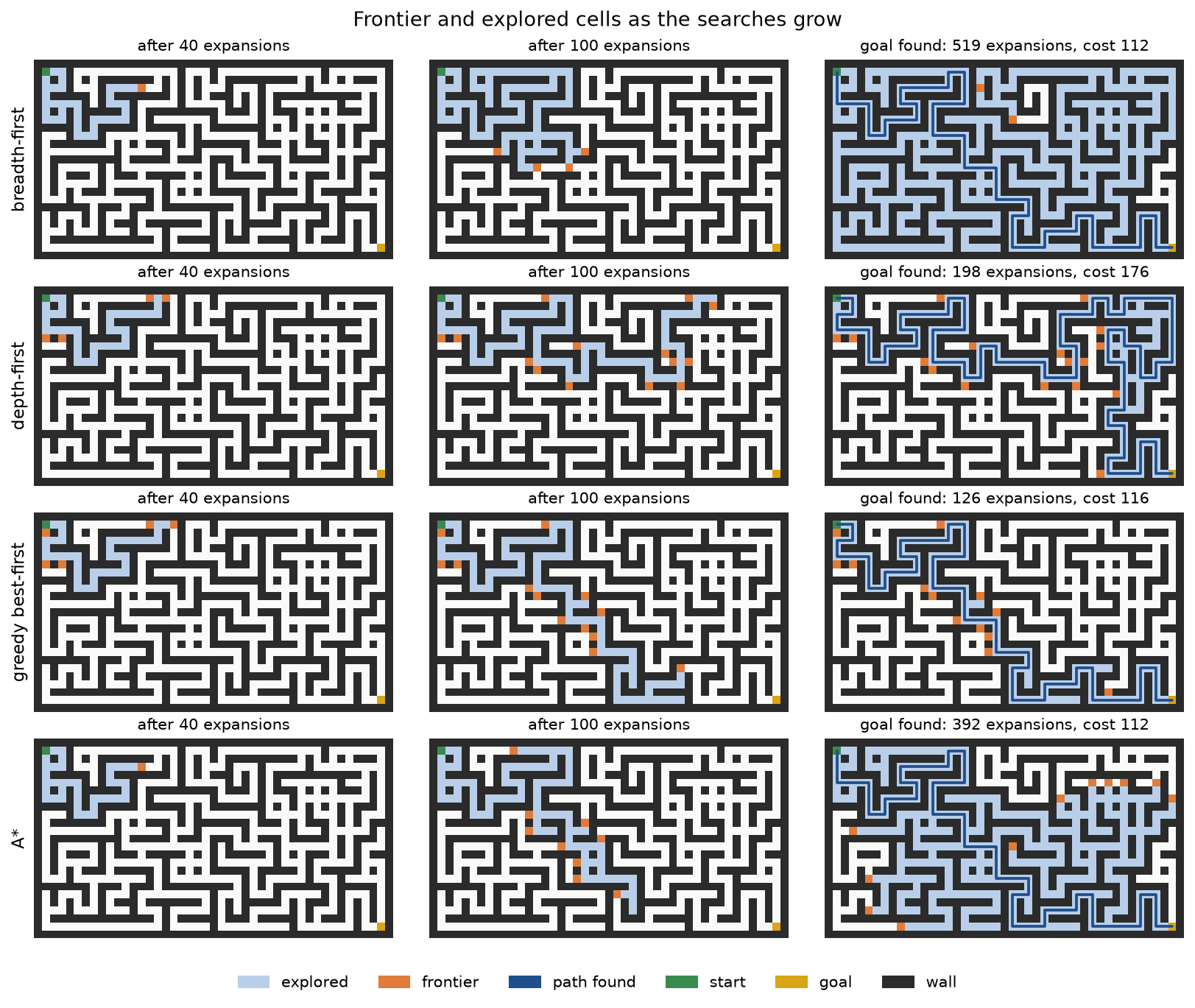
The snapshots show the shapes of the strategies: an even flood for breadth-first search, a single probing line for depth-first search, a beeline for greedy search and a flood leaning towards the goal for A. In a maze the walls make the Manhattan distance a weak guide, so A saves a quarter of the expansions on this maze and 40 % over all fifty.

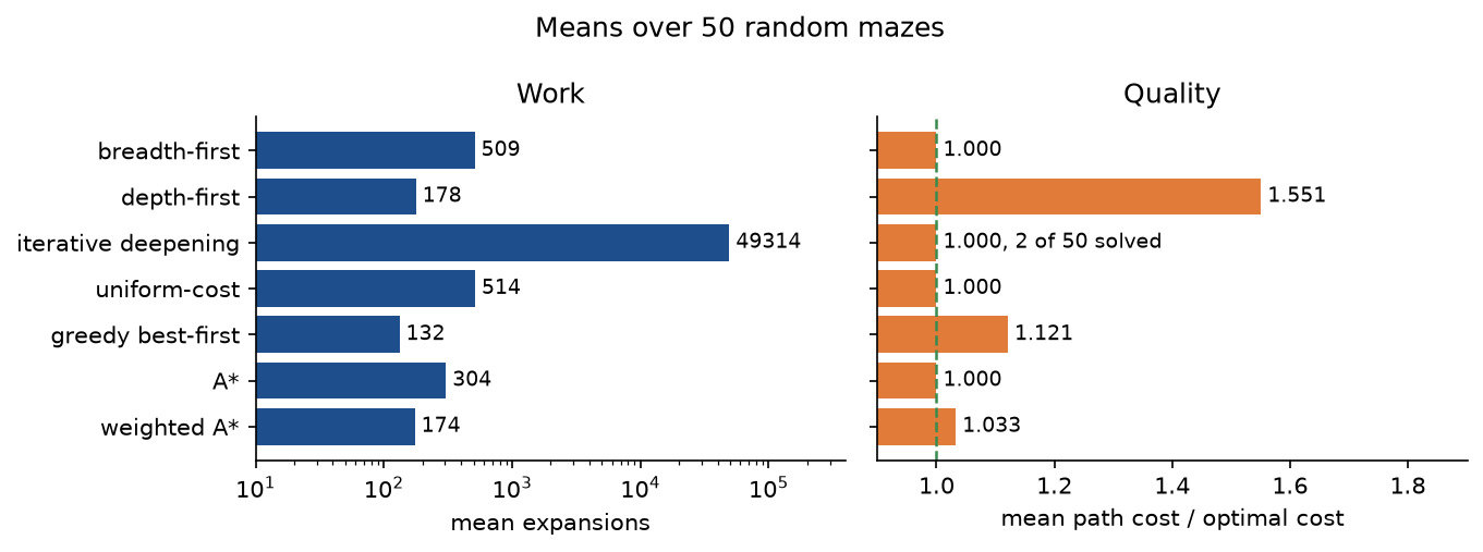
The summary is the trade-off of the whole page in one picture: the algorithms that spend least either give up optimality, like greedy and depth-first search, or bound the loss, like weighted A*. With --loops 0 every maze has exactly one route, so every algorithm that finds it is optimal, and iterative deepening solves 37 of the 50 mazes within its budget: in a tree every cell has a single path, so each iteration costs at most one pass over the maze, and only the mazes with the longest routes need more passes than the budget allows.

The notebook search_algorithms.ipynb is a guided tour in the order of this page: the road network traced by every algorithm, the small maze, the 8-puzzle example, one section per pitfall, the generated maze with its snapshots, the heuristics on an open grid and weighted A*, the effective branching factor measurements and the comparison with networkx. The tests in tests check the worked examples value by value, the mathematical properties above and the agreement with networkx, and run in a few seconds:

python -m pytest foundations/search-algorithms

Every maze, grid, road network and puzzle board is generated from a seed, so nothing is downloaded and no licence is involved.

In practice

networkx implements Dijkstra's algorithm and A* for weighted graphs. to_networkx sweeps the reachable states of any problem into a networkx.DiGraph with edge weights, and the library computes the cost of the best path:

import networkx as nx

from search_algorithms import octile, random_grid, to_networkx

maze = random_grid(30, 40, 0.22, seed=1, diagonal=True)
graph = to_networkx(maze)
nx.dijkstra_path_length(graph, maze.start, maze.goal, weight="weight")
nx.astar_path_length(graph, maze.start, maze.goal, heuristic=octile, weight="weight")

examples/compare_with_networkx.py runs this on 120 random 30 by 40 grids, 4- and 8-connected, half of them with cells that cost 1 to 4 to enter. 106 of them have a route; on those the largest difference between our uniform-cost search and nx.dijkstra_path_length is 7.1 × 10⁻¹⁵ and between our A* and nx.astar_path_length 5.7 × 10⁻¹⁴, floating-point rounding of sums that contain √2, and both sides agree that the other 14 have none. On 30 random road networks with 300 places and 900 roads, uniform-cost search matches nx.dijkstra_path_length exactly, and the breadth-first route has as many roads as nx.shortest_path_length reports on all 30. tests/test_comparisons.py repeats the check on smaller instances.

When to use which:

• Breadth-first search for unweighted problems that fit in memory, and as a sweep that labels every state with its distance, as the 8-puzzle measurement does.
• Uniform-cost search, which is Dijkstra's algorithm, for weighted problems without a useful heuristic, and when distances to many states are needed. scipy.sparse.csgraph.dijkstra computes all of them on a sparse matrix.
• A* with a consistent heuristic for a single start and goal. Design the heuristic as the exact cost of a relaxed problem and take the maximum of several when they are cheap to compute.
• Iterative deepening, or its heuristic version IDA*, when memory is the binding constraint and the space is tree-like. On graphs full of cycles, such as mazes with loops, it repeats so much work that it is hopeless, as the project shows.
• Weighted A when a slightly longer path found much sooner is acceptable; anytime variants such as ARA start with a large weight and lower it while time remains.
• On large road networks, precomputation beats any online heuristic: contraction hierarchies or landmark-based heuristics answer queries in milliseconds. On uniform grids, jump point search skips symmetric paths.

Our implementations are for learning and for small problems: they keep a Python object per node and generate a few hundred thousand nodes per second on a laptop. networkx is the convenient choice for graphs that fit in memory, and compiled libraries or the techniques above take over at scale.

Mobile robots plan on costmaps with exactly these algorithms: a global planner runs Dijkstra's algorithm or A* over an occupancy grid with inflated obstacles, and Navigation builds on this page. Value iteration in Markov decision processes generalises shortest paths to random transitions, adversarial search in game-playing agents adds an opponent, beam search in decoding strategies is a memory-bounded best-first search, and edit distance is a shortest path in a grid graph.

Pitfalls

• Testing the goal when a node is generated. Uniform-cost search and A* must test a node when it leaves the frontier. Testing on generation returns the first path to reach the goal, S, C, G at cost 17 in the worked example instead of 11, as examples/common_mistakes.py prints. The early test is correct only for breadth-first search.
• A first-in first-out queue or a max-heap instead of a min-priority queue. Dijkstra's algorithm needs a frontier that always returns the entry with the smallest cost. Some descriptions call the structure a max-heap; with one, the search removes the most expensive path first. A queue that ignores the priorities turns uniform-cost search into breadth-first search and returns S, C, G at cost 17, as constant_priority_search shows. Python's heapq is a min-heap.
• Using breadth-first search on weighted problems. It minimises the number of actions, not their cost: two roads costing 17 against five costing 11 in the worked example.
• Forgetting the explored set. Tree search on a graph with cycles repeats states. On the small maze breadth-first tree search expands 244 nodes where graph search expands 16, and depth-first tree search without a cycle check alternates between two cells until a budget of 10,000 expansions runs out, as examples/small_maze.py shows. Conversely, depth-first graph search stores every explored state; the O(bm) memory belongs to the tree-search version only.
• Believing that admissibility is always enough. A with an admissible heuristic is optimal as tree search or as graph search that reopens closed states; the closed-set version that never reopens needs consistency. Statements that A is optimal with any admissible heuristic leave out which version is meant.

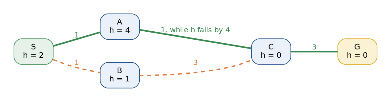
Here h never overestimates, but it drops by 4 across the road from A to C of cost 1, and by 2 across the road from A back to S. A* closes C through B at cost 4, ignores the cheaper path through A when it arrives and returns cost 7 instead of 5; reopening C finds the optimum. examples/common_mistakes.py prints both runs.

• Stating A without its conditions. A is not optimal with an arbitrary heuristic. One overestimate on the worked example, h(D) = 8, returns a route costing 12 instead of 11. Check admissibility, ideally consistency, before relying on optimality; admissibility_violations and consistency_violations do it for any problem small enough to sweep.
• Using the Manhattan distance with diagonal moves. It overestimates every diagonal step. On the open grid A* with it returns a path of cost 85.1127 instead of 83.9411; the octile distance is the matching heuristic, as examples/grid_heuristics.py shows. The same mistake appears when costs are scaled, for example when cells cost 0.5 to cross but the heuristic counts cells: multiply by the cheapest cost per move.
• Breaking ties badly. On an open 40 by 40 grid every cell between start and goal has f = 78 under the Manhattan distance. Breaking ties first in, first out expands 1599 cells; preferring the smaller h expands 78.

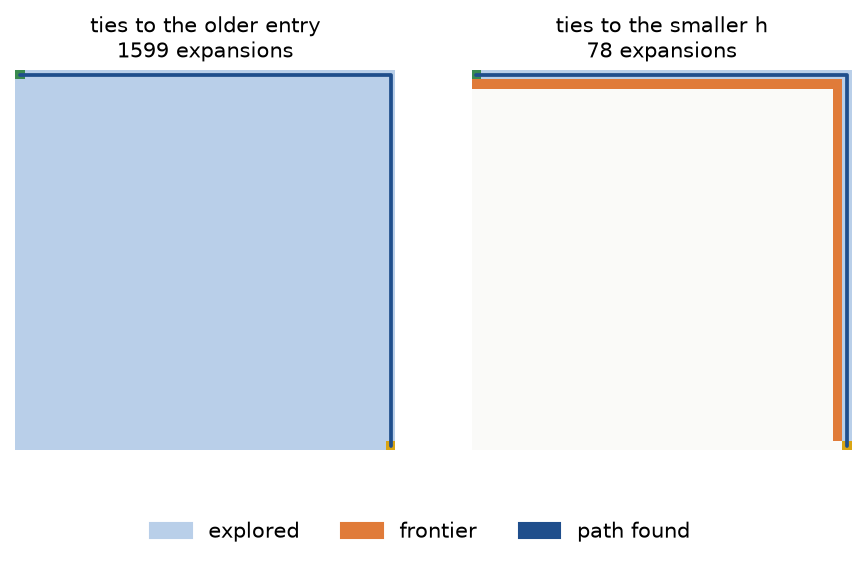
Both runs return a path of cost 78; only the work differs, by a factor of twenty.

• Comparing floating-point path costs exactly. With diagonal costs, two equally long routes can differ in the last bit. On a 40 by 60 grid an exact comparison made A* reopen 4 closed states for nothing and expand 927 cells instead of 923; a relative tolerance of 10⁻⁹ removes the reopenings, as examples/common_mistakes.py prints.
• Reading meaning into the answer of depth-first search. Its route depends on the order in which actions are listed: the alphabetical order happens to give the cheapest route on the worked example, the reverse order gives cost 17, as examples/road_network.py prints with ReversedActions.
• Comparing effective branching factors computed differently. b depends on whether N counts generated or expanded nodes, includes the root, and includes states re-added with a cheaper path. For the same run of A with h2 on the 8-puzzle example, 36 generated nodes give 1.1608, 37 with the root give 1.1647, 21 expanded nodes give 1.0835 and 22 with the root give 1.0903. Compare only numbers computed the same way; this page counts generated nodes without the root.

Further reading

• S. Russell and P. Norvig, Artificial Intelligence: A Modern Approach, fourth edition, Pearson, 2020, chapter 3. Problem formulation, uninformed and informed search, and heuristic design.
• P. E. Hart, N. J. Nilsson and B. Raphael, "A formal basis for the heuristic determination of minimum cost paths", IEEE Transactions on Systems Science and Cybernetics 4(2), 100-107, 1968. The paper that introduced A*.
• E. W. Dijkstra, "A note on two problems in connexion with graphs", Numerische Mathematik 1, 269-271, 1959.
• R. E. Korf, "Depth-first iterative-deepening: an optimal admissible tree search", Artificial Intelligence 27(1), 97-109, 1985.
• J. Pearl, Heuristics: Intelligent Search Strategies for Computer Problem Solving, Addison-Wesley, 1984. Relaxed problems, dominance and the analysis of A*.
• R. Dechter and J. Pearl, "Generalized best-first search strategies and the optimality of A*", Journal of the ACM 32(3), 505-536, 1985.
• A. Martelli, "On the complexity of admissible search algorithms", Artificial Intelligence 8(1), 1-13, 1977. Re-expansions under inconsistent heuristics.
• I. Pohl, "Heuristic search viewed as path finding in a graph", Artificial Intelligence 1(3-4), 193-204, 1970. Weighting the heuristic.
• M. Likhachev, G. Gordon and S. Thrun, "ARA: anytime A with provable bounds on sub-optimality", Advances in Neural Information Processing Systems 16, 2003.
• J. C. Culberson and J. Schaeffer, "Pattern databases", Computational Intelligence 14(3), 318-334, 1998.
• A. Reinefeld, "Complete solution of the eight-puzzle and the benefit of node ordering in IDA*", IJCAI 1993. The 31-move maximum.
• D. Harabor and A. Grastien, "Online graph pruning for pathfinding on grid maps", AAAI 2011. Jump point search.
• T. H. Cormen, C. E. Leiserson, R. L. Rivest and C. Stein, Introduction to Algorithms, fourth edition, MIT Press, 2022, chapter 22. Single-source shortest paths, Dijkstra's algorithm and Bellman-Ford.