Regularization

A network with far more parameters than training examples can fit the training set perfectly, noise included, and then predict new data badly. Regularization is everything we do to a learning procedure to lower its error on new data rather than on the training data: penalties on the size of the weights, noise injected during training, stopping before the optimizer is done, and more varied training data. This page derives the L2 penalty twice, as an extra gradient term and as a Gaussian prior, explains why it is not the same as weight decay inside Adam, derives the sparsity of L1, works out dropout with a fresh mask per mini-batch, inverted scaling and the switch between training and evaluation, and connects early stopping to L2. One training step of a small network is worked by hand with each regularizer, everything is implemented in NumPy, the common dropout mistakes are demonstrated, and a sample project compares five regularizers on 200 handwritten digits with every strength chosen on validation data and checked on a test set. Afterwards you will be able to add each regularizer to a backward pass yourself, choose between them, and recognise the mistakes that silently turn them off or make them harmful. It builds on Backpropagation.

To run the code in this topic, install the base and ml groups, and the deep group for the comparisons with PyTorch.

Intuition

Fifteen noisy points from a sine curve and a network with 1,153 parameters: the left panel below shows what happens. Trained to convergence without any regularization, the network passes through every training point and swings wildly between them. Its training cost falls to 0.0002 while its cost on 100 fresh points from the same curve rises to 0.4429, more than twenty times the 0.02 that the noise alone would cost. That is overfitting. The right panel shows its signature over time: the training cost keeps falling, while the validation cost falls for a while and then turns upwards as the network starts to fit the noise.

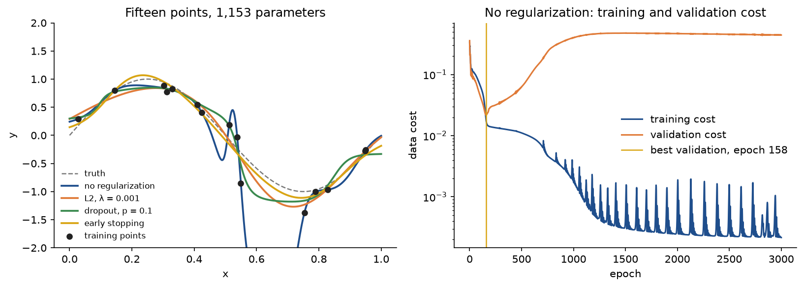
Three remedies appear in the same figure. An L2 penalty keeps the weights small, and a network with small weights cannot produce steep swings. Dropout trains the network while randomly silencing hidden units, so no unit can rely on a particular partner and the function it learns is smoother. Early stopping keeps the network from the epoch where the validation cost was lowest, before the swings developed. Each brings the fitted curve close to the truth.

The methods fall into four families, all of which trade a little fit on the training data for better behaviour on new data:

• Penalize the parameters. The L2 penalty, also known as weight decay, and the L1 penalty add a cost for large weights, so the optimizer prefers simpler solutions.
• Inject noise into training. Dropout, input noise, label smoothing and, as a side effect, batch normalization make the training problem harder in a way the network can only solve by being robust.
• Limit the optimization. Early stopping ends training before the network has had time to fit the noise.
• Enlarge the data. Data augmentation adds label-preserving variations of the training examples.

The diagram shows where each one acts in a training step. The amber boxes are the places a regularizer enters: augmentation changes the batch, dropout changes the forward pass and with it the backward pass in orange, label smoothing changes the targets of the data cost, and a penalty adds its gradient before the update. After every epoch the validation cost decides whether training continues, and the network finally returned is the best one seen, evaluated with nothing dropped.

How it works

Notation

The notation of Backpropagation carries over unchanged. Layers are numbered from 0, the inputs, to L, the outputs. The weight matrix W of layer l has one row per unit of layer l and one column per unit of layer l - 1, so its entry in row j and column k is the weight to unit j from unit k. The net inputs z = W a + b and the activations a = f(z) of layer l are computed from the activations a of layer l - 1, the error δ of a unit is the derivative of the cost with respect to its net input, and a mini-batch stores one example per row in the matrices Z, A and Δ. The four equations B1 to B4 turn the output error into the errors of every layer and the gradients of every parameter. As there, formula images write the layer as a superscript in parentheses, and the text writes W1, b1, A1 and Δ1 for the weights, biases, activations and errors of layer 1, and likewise for layer 2. New quantities on this page:

• The data cost C0 is the average per-example cost over the training set or a mini-batch, the cost C of the backpropagation page.
• The penalty Ω measures the size of the weights: half the sum of their squares for L2, the sum of their absolute values for L1. Biases are not included.
• The strength λ ≥ 0 scales the penalty, and the regularized cost is C = C0 + λΩ.
• The learning rate is η, the number of training examples n and the mini-batch size m.
• Dropout drops a unit of layer l with probability p and keeps it with probability q = 1 - p. Its mask r holds one independent entry per unit, 1 with probability q and 0 otherwise, and ã holds the activations after dropout, the values the next layer actually receives. For a mini-batch the masks and the dropped activations form the matrices R and Ã, one row per example.
• H is the Hessian of the data cost at its minimum w*, with eigenvalues h and orthonormal eigenvectors u.
• τ counts gradient-descent steps, ε is the label-smoothing amount and K the number of classes.

Both penalties sum over the weights of every layer and over no bias, and the regularized cost adds one of them, scaled by its strength, to the data cost.

Overfitting and generalization

The quantity we care about is the expected cost on new examples drawn from the same distribution as the training data. The training cost is only an estimate of it, and a biased one, because the parameters were chosen to make it small. The difference between the two is the generalization gap. It grows with the flexibility of the model and shrinks with the number of training examples: with 15 points and 1,153 parameters there are many settings of the weights that fit the points exactly, and nothing in the data says which of them is right between the points. Regularization adds a preference among the solutions that fit, for small weights, for robustness to noise or for solutions reached early from a small initialization, and that preference decides how the network behaves away from the training data. The preference cannot be checked on the training data itself, so every regularization strength is chosen on held-out validation data, and the final verdict comes from a test set that played no part in any choice.

L2 regularization as a gradient term

Add λ times half the sum of squared weights to the cost. The penalty does not depend on any net input, so the forward pass, the errors δ and equations B1 to B3 are unchanged. Differentiating the penalty with respect to one weight leaves λ times that weight, so B4 gains a term and the bias gradient does not:

A gradient step with learning rate η then reads

Every step first shrinks each weight by the factor 1 - ηλ and then takes the ordinary data step, hence the name weight decay. A weight that the data do not push on decays geometrically, to (1 - ηλ) to the power t of its starting value after t steps, which requires 0 < ηλ < 1. On a mini-batch the data gradient is the batch average from the backpropagation page, an unbiased estimate of the gradient of the training-set average, while the penalty term is exact and applied in full at every step.

Conventions differ by a factor. Some texts write the penalty as λ/(2n) times the sum of squares next to an average data cost, so their λ is n times ours and their decay factor is 1 - ηλ/n; others sum the data cost over the examples instead of averaging it. PyTorch's weight_decay in SGD and Adam is the λ used here. With the λ/(2n) convention, keeping λ fixed while the training set grows weakens the penalty, which matches the prior reading below.

Biases are left out. A bias shifts one unit's net input and does not interact with the inputs; there are few of them, penalizing them restricts the network little and can push units into the wrong operating region. The same holds for the scale and shift parameters of normalization layers.

L2 as a Gaussian prior

Read the data cost as an average negative log-likelihood. Cross-entropy is exactly that for a softmax output, and the squared error is that for Gaussian noise of unit variance, up to a constant. Put an independent Gaussian prior with mean zero and variance σ² on every weight. By Bayes' rule the log of the posterior is the log-likelihood plus the log-prior plus a constant, and its most probable value, the maximum a posteriori estimate, minimizes minus 1/n times it:

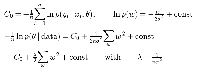
Minimizing the L2-regularized cost is finding the most probable weights under a zero-mean Gaussian prior. A narrower prior, a smaller σ, means a stronger penalty, and with a fixed prior the penalty matters less as the data grow, as it should: with enough evidence the data overrule the prior.

What L2 does to the solution

Near the unregularized minimum w* the data cost is approximately quadratic, with the symmetric positive semidefinite Hessian H. Setting the gradient of the regularized cost to zero gives the regularized minimum w̃, and writing it along the eigenvectors u of H shows what happens in each direction separately:

Directions in which the cost curves steeply, h much larger than λ, are those the data determine well, and they are left almost untouched. Directions in which the cost is nearly flat, h much smaller than λ, are those the data barely constrain, and there the solution is pulled almost to zero. L2 removes exactly the components of the weights that the training data cannot justify. Linear regression derives the same shrinkage factors from the singular values of the data matrix for ridge regression.

L1 regularization and sparsity

The L1 penalty is λ times the sum of the absolute weights. Away from zero its derivative is λ sgn w, so the step is

L1 subtracts the same amount ηλ from every weight, whatever its size, while L2 subtracts ηλ times the size of the weight. For equal λ, L1 shrinks weights smaller than one in magnitude harder than L2 does and larger weights more gently. The prior reading carries over: a Laplace prior, with density proportional to exp(-|w|/β), gives λ = 1/(nβ), and the Laplace density has a sharp peak at zero where the Gaussian is flat.

The peak is what produces exact zeros. Take one weight whose data cost is the quadratic h/2 (w - w*)² with h > 0, and minimize it together with λ|w|:

For positive w the derivative vanishes at w - λ/h, which is positive only if w exceeds λ/h, and symmetrically for negative w. In between, the derivative is negative just left of zero and positive just right of it, so the minimum sits at the corner: formally, zero belongs to the subgradient, the set of slopes the kink allows, exactly when |w*| ≤ λ/h. Together:

The L1 solution is soft-thresholding: every weight whose unregularized value is smaller than λ/h becomes exactly zero, and the others move towards zero by λ/h. The L2 solution is a rescaling and is never zero unless w* is. With a diagonal Hessian this holds weight by weight; in general L1 still produces exact zeros, which is why it is used for feature selection and compression.

Plain gradient descent does not find those zeros. A step of size ηλ jumps over zero and back, so the weights end up oscillating around zero with an amplitude up to ηλ: small, but not zero. The proximal step does better. It takes the data step to an intermediate value w′ and then minimizes (w - w′)²/(2η) + λ|w|, which by the derivation above with h = 1/η is

A weight that the data step leaves within ηλ of zero lands on zero and stays there until the data gradient is strong enough to pull it out.

Weight decay in adaptive optimizers

For plain SGD, adding λW to the gradient and multiplying the weights by 1 - ηλ are the same thing, as the L2 derivation showed. For adaptive methods they are not. Adam keeps running averages m and v of each parameter's gradient g and squared gradient, corrects them for their start at zero and divides one by the square root of the other:

Everything acts entry by entry, usually with β1 = 0.9, β2 = 0.999 and a small constant of 10⁻⁸ in the denominator. Optimizers covers Adam itself. With an L2 penalty the gradient is the data gradient plus λθ, and the decay term is divided by the square root of v̂ along with everything else. Three consequences follow.

• On the first step m̂ = g and v̂ = g², so the update is η g/(|g| + 10⁻⁸), almost exactly η sgn g. Every parameter moves by the learning rate, and the penalty matters only if λθ is large enough to flip the sign of the gradient.
• A parameter with no data gradient has g = λθ. Then m scales with λ and the square root of v scales with λ, and while the constant in the denominator is negligible their ratio does not depend on λ at all: the strength of the penalty cancels, and the parameter is driven to zero at roughly the learning rate per step, whether λ is tiny or large.
• A parameter with large data gradients has a large v̂, so its decay, λθ divided by the square root of v̂, is small. The weights that the data use most are decayed least.

Decoupled weight decay, the method behind AdamW, applies the decay outside the adaptive step, with gradients of the data cost only:

Every weight shrinks by the same factor per step, exactly as weight decay does under SGD. In PyTorch, Adam(weight_decay=λ) and SGD(weight_decay=λ) add λθ to the gradient, while AdamW(weight_decay=λ) multiplies the weights by 1 - ηλ. The decay is then tied to the learning rate: the per-step decay is the product ηλ, so a learning-rate schedule also schedules the decay, and with η = 10⁻³ the default λ = 0.01 removes only 10⁻⁵ of each weight per step. The original formulation scales the decay by the schedule multiplier but not by the base learning rate, so values of λ do not transfer between the two.

Dropout

Dropout changes the network during training instead of the cost. For every example in every training step, each unit of a layer with drop probability p is silenced independently with that probability. Inverted dropout divides the survivors by the keep probability q:

The scaling keeps every unit's expected contribution unchanged:

Since the next net input is linear in ã, its expectation over the mask is the net input of the full network. At evaluation time no unit is dropped and nothing is scaled. Drop probabilities are usually 0.5 for wide hidden layers in the original setting, 0.1 to 0.3 in many modern networks, and 0.2 or less on the inputs, if the inputs are dropped at all.

The backward pass follows from the chain rule. The net input of a unit now reaches the next layer through r f(z)/q, whose derivative is r f′(z)/q, so B2 gains the factor r/q; and the weights of layer l + 1 multiply ã, so B4 uses the dropped activations:

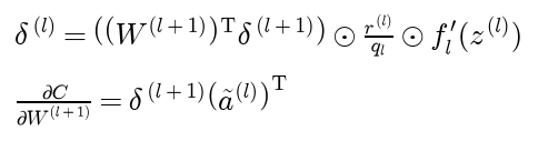
B1 and B3 are unchanged. A dropped unit has r = 0, so its error is zero and its incoming weights and bias learn nothing from that example; its outgoing weights see ã = 0 and learn nothing either. For a mini-batch the masks form a matrix R with an independent entry for every example and unit, and the batch equations of the backpropagation page become

A new R is drawn for every mini-batch; libraries draw one on every forward call in training mode. The forward and backward pass of one step must use the same mask, and a gradient check must hold the mask fixed.

The older formulation, sometimes called classic dropout, trains with the bare mask and multiplies the outgoing weights by q for evaluation, so that each evaluation net input equals its expected value during training:

A network trained with inverted dropout and weights W computes the same functions as one trained with classic dropout and weights W/q; the inverted form is preferred because the evaluation network needs no change.

Dropout as an ensemble

A network with N droppable units contains 2 to the power N subnetworks, one for each mask, all sharing the same weights. Each training step trains a randomly chosen subnetwork on each example, so dropout trains an exponentially large ensemble with weight sharing. The ensemble's prediction would average the subnetworks, each weighted by the probability of its mask:

Evaluating the full network approximates that average, and in two cases exactly.

• If the dropped layer feeds a linear output directly, the output is linear in ã, so the probability-weighted average of the subnetworks' outputs is the output of the full network. The worked example below enumerates all eight subnetworks and finds exactly that.

The middle step is the expectation of ã computed above.

• If the dropped layer feeds a softmax output, take the probability-weighted geometric mean of the subnetworks' class probabilities and renormalize. The softmax denominator of each subnetwork is the same for every class, so it disappears in the renormalization, and what remains for class k is

so the renormalized geometric mean is the softmax of the expected net inputs, again the output of the full network, as tests/test_dropout.py checks.

With nonlinear layers between the mask and the output the full network is only an approximation of the ensemble, the weight-scaling inference rule, but a good one in practice. Averaging the outputs of many sampled masks at evaluation time, Monte Carlo dropout, gives another estimate and a measure of uncertainty from the spread.

Early stopping

Train while measuring the cost on a validation set after every epoch. Keep a copy of the parameters with the lowest validation cost so far, and stop when it has not improved for a fixed number of epochs, the patience. Return the best copy, not the last parameters. Early stopping turns the number of training steps into a hyperparameter chosen on validation data in a single run, which also means the validation set has been used for a choice and cannot serve as the final test.

For a quadratic cost early stopping is close to an L2 penalty. Start gradient descent at zero. Each step moves against the gradient H(w - w*), so the distance to the minimum is multiplied by I - ηH per step, and along each eigenvector by 1 - ηh:

Both start at zero and approach w* along the steep directions first. For a small step the power is close to an exponential, and with x = h/λ and λ = 1/(ητ) the two factors become 1 - e to the power -x and x/(1 + x):

Both factors are x to first order for small x, and both tend to 1 for large x, so training for τ steps acts like an L2 penalty of strength λ ≈ 1/(ητ). In between the match is approximate: the two factors differ by at most 0.2036, at x ≈ 2.51, as examples/overfitting_and_early_stopping.py prints and tests/test_shrinkage.py checks. The figure shows both paths on a two-dimensional quadratic with curvatures 1 and 0.05 along two directions rotated by 30 degrees, learning rate 0.1 and the minimum at (1, 1).

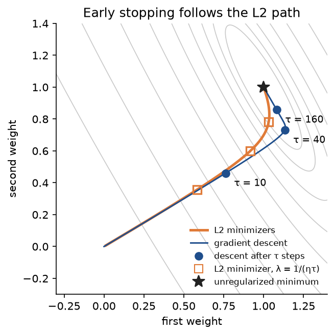
After 10, 40 and 160 steps the descent sits at distances 0.2067, 0.2531 and 0.0894 from the L2 minimizer with λ = 1/(ητ), and both paths bend from the steep direction towards the flat one. Early stopping finds its strength in one run, while L2 needs a run per value of λ; L2, on the other hand, keeps acting however long training continues.

Data augmentation

Augmentation trains on transformed copies T(x) of the training inputs with unchanged labels, with T drawn at random from a family of transformations that do not change the label: small shifts, rotations, crops and scalings, colour and brightness changes, flips where they do not change the class, noise. The training cost becomes an average over the transformations:

This tells the network about invariances the task is known to have, and adds examples from roughly the right distribution. Transformations are drawn afresh in every epoch, so the network never sees exactly the same input twice. Two conditions matter. The transformations must preserve the label: a 6 rotated by 180 degrees is a 9, and a mirrored digit is often no digit at all. And augmentation must happen after the data are split, on the training side only. Augmenting first puts near copies of the same original on both sides of the split and inflates every score; Data leakage and pitfalls treats this and related leaks.

Noise injection and label smoothing

Adding noise to the inputs is a regularizer in its own right. For a linear model with the squared error and input noise ξ of mean zero and covariance σ² times the identity, expand the square and take the expectation:

The middle term vanishes because the noise has mean zero, and the last term is the noise covariance seen through w. Training on noisy inputs therefore minimizes, on average, the L2-regularized cost with λ = σ². For a network, a similar expansion gives a penalty on how fast the output changes with the input, and dropout is multiplicative noise on the hidden units.

Label smoothing adds noise to the targets instead. With K classes, the one-hot target y is replaced by

For a softmax output with cross-entropy, B1 still gives the output error a - y with the smoothed target, because that shortcut holds for any target that sums to one. The cost is smallest when the output equals the smoothed target, so the net inputs of a perfectly fitted example stop growing once the correct class leads every other by a fixed gap:

With hard targets the same gap grows without limit on training data the network can separate, and that growth is what makes unregularized classifiers overconfident. With ε = 0.1 and ten classes the network is taught never to give the correct class more than 0.91. torch.nn.CrossEntropyLoss(label_smoothing=ε) uses this definition. Loss functions covers softmax and cross-entropy.

Batch normalization as a side effect

Batch normalization standardizes each unit's net input with the mean and variance of the current mini-batch. In training mode one example's output therefore depends on the other examples that happen to share its batch, which adds noise of a kind similar to dropout and has a mild regularizing effect that weakens as batches grow. In evaluation mode the layer uses running averages collected during training and is deterministic, the same switch dropout needs. The regularization is a side effect; batch normalization is used because it makes deep networks easier to optimize, and it does not replace a deliberate regularizer.

Worked example

The network has two inputs, three ReLU hidden units and one linear output, and is trained with the squared-error data cost on a batch of m = 2 examples, with learning rate η = 0.2 and strength λ = 0.1 for both penalties, so that ηλ = 0.02. For the dropout step the hidden units are dropped with probability p = 0.5.

The diagram gives every parameter. As matrices, the hidden weights W1 have rows (0.3, -0.3), (-0.2, -0.1) and (0.2, -2.0), one row per hidden unit; the hidden biases b1 are (0.2, 0.5, 0.1); the output weights W2 form the single row (-0.5, 1.0, 0.2); and the output bias b2 is 0.2. The two examples, the rows of X, are (-1, -1) and (1, -1), with targets 0 and 1. All the arithmetic is exact in a few decimal places, so every value below can be checked on paper.

Forward pass and data gradient

For example 1 and hidden unit 1 the net input is 0.3 × (-1) + (-0.3) × (-1) + 0.2 = 0.2. Every hidden net input is positive, so the ReLU passes them unchanged and its derivative is 1 everywhere:

• Example 1: hidden net inputs and activations (0.2, 0.8, 1.9), output 1.28, cost 0.8192.
• Example 2: hidden net inputs and activations (0.8, 0.4, 2.3), output 0.66, cost 0.0578.

For example 1 the output is -0.5 × 0.2 + 1.0 × 0.8 + 0.2 × 1.9 + 0.2 = 1.28. Each cost is half the squared difference between output and target, 1.28² / 2 = 0.8192 and 0.34² / 2 = 0.0578, so the data cost is C0 = 0.4385.

The output is linear, so B1 gives the output errors Δ2 = A2 - Y = (1.28, -0.34), one per example. B2 sends each error back along W2, and with ReLU derivatives of 1 the hidden errors Δ1 are (-0.64, 1.28, 0.256) for example 1 and (0.17, -0.34, -0.068) for example 2. B3 and B4 average over the two examples:

• Output layer: the gradient of W2 is (-0.008, 0.444, 0.825) and the gradient of b2 is 0.47. The first entry, for instance, is (1.28 × 0.2 - 0.34 × 0.8) / 2 = (0.256 - 0.272) / 2 = -0.008.
• Hidden layer: the gradient of W1 has rows (0.405, 0.235), (-0.81, -0.47) and (-0.162, -0.094), and the gradient of b1 is (-0.235, 0.47, 0.094).

The L2 step

The penalty is half the sum of the nine squared weights, (0.09 + 0.09 + 0.04 + 0.01 + 0.04 + 4 + 0.25 + 1 + 0.04) / 2 = 5.56 / 2 = 2.78, so the regularized cost is 0.4385 + 0.1 × 2.78 = 0.7165. Most of the penalty comes from the single weight -2. The weight gradients gain λW: the gradient of W1 becomes the rows (0.435, 0.205), (-0.83, -0.48) and (-0.142, -0.294), and that of W2 becomes (-0.058, 0.544, 0.845).

The step multiplies every weight by 1 - ηλ = 0.98 and then takes the data step. Next to the step without a penalty:

• Without a penalty, W1 becomes the rows (0.219, -0.347), (-0.038, -0.006) and (0.2324, -1.9812).
• With L2, W1 becomes the rows (0.213, -0.341), (-0.034, -0.004) and (0.2284, -1.9412), and W2 becomes (-0.4884, 0.8912, 0.031).

For the bottom-right weight, 0.98 × (-2) - 0.2 × (-0.094) = -1.96 + 0.0188 = -1.9412. The biases take the same step in both cases.

The L1 step

The sum of the absolute weights is 4.8, so the regularized cost is 0.4385 + 0.1 × 4.8 = 0.9185. The weight gradients gain λ sgn W, plus or minus 0.1: the gradient of W1 becomes the rows (0.505, 0.135), (-0.91, -0.57) and (-0.062, -0.194).

• The subgradient step moves every weight 0.02 further towards zero than the plain step, so W1 becomes the rows (0.199, -0.327), (-0.018, 0.014) and (0.2124, -1.9612).
• The proximal step soft-thresholds the plain step at ηλ = 0.02: every entry larger than 0.02 in magnitude loses 0.02, and the one entry smaller than that, -0.006, becomes exactly zero. W1 becomes the rows (0.199, -0.327), (-0.018, 0) and (0.2124, -1.9612).

Two weights show the difference between the penalties:

• The large weight in row 3 and column 2 of W1 starts at -2. The plain step takes it to -1.9812, the L2 step to -1.9412, and both L1 steps to -1.9612.
• The small weight in row 2 and column 2 starts at -0.1. The plain step takes it to -0.006, the L2 step to -0.004, the L1 subgradient step to +0.014 and the proximal step to exactly 0.

L2 pulls the large weight 0.04 towards zero, twice as far as L1's 0.02, and the small weight only 0.002, a tenth of L1's pull. On the small weight the L1 subgradient step overshoots: it crosses zero and lands at +0.014, and the next L1 step pushes it back by 0.02 in the other direction. The proximal step stops it at zero.

A dropout step

Now drop hidden units with probability p = 0.5, so survivors are multiplied by 1/q = 2. Example 1 keeps units 1 and 3, and example 2 keeps units 2 and 3, so the mask R1 has rows (1, 0, 1) and (0, 1, 1).

Each example trains its own thinned network. The dropped activations Ã1 have rows (0.4, 0, 3.8) and (0, 0.8, 4.6), and the outputs are 0.76 and 1.92: for example 1, -0.5 × 0.4 + 0.2 × 3.8 + 0.2 = 0.76. The costs are 0.76² / 2 = 0.2888 and 0.92² / 2 = 0.4232, so this step's data cost is 0.356. The output errors are (0.76, 0.92). B2 first sends them back along W2, giving the rows (-0.38, 0.76, 0.152) and (-0.46, 0.92, 0.184), and then multiplies them entry by entry by R1/q, whose rows are (2, 0, 2) and (0, 2, 2):

• The hidden errors Δ1 have rows (-0.76, 0, 0.304) and (0, 1.84, 0.368).
• B4 uses the dropped activations Ã1: the gradient of W2 is (0.152, 0.368, 3.56) and that of b2 is 0.84.
• The gradient of W1 has rows (0.38, 0.38), (0.92, -0.92) and (0.032, -0.336), and that of b1 is (-0.38, 0.92, 0.336).

Unit 1 learns only from example 1 and unit 2 only from example 2. In the outgoing weights, the entry for unit 1 is 0.76 × 0.4 / 2 = 0.152, because example 2 contributes 0.92 × 0 = 0. On the next mini-batch a new R1 decides which units learn from which examples.

The ensemble behind the evaluation output

At evaluation time no unit is dropped and nothing is scaled, so the network outputs 1.28 and 0.66, the values of the plain forward pass. With three hidden units there are eight subnetworks, each with probability 1/8 when q = 0.5. Each kept unit contributes twice its normal amount: for example 1, unit 1 adds 2 × (-0.5 × 0.2) = -0.2, unit 2 adds 2 × 0.8 = 1.6 and unit 3 adds 2 × 0.38 = 0.76, on top of the bias 0.2. The outputs of the eight subnetworks for examples 1 and 2 are:

• No unit kept: 0.2 and 0.2.
• Unit 3 kept: 0.96 and 1.12.
• Unit 2 kept: 1.8 and 1.0.
• Units 2 and 3 kept: 2.56 and 1.92.
• Unit 1 kept: 0 and -0.6.
• Units 1 and 3 kept: 0.76 and 0.32.
• Units 1 and 2 kept: 1.6 and 0.2.
• All three kept: 2.36 and 1.12.

The averages are 10.24 / 8 = 1.28 and 5.28 / 8 = 0.66: because the output is linear, the full network in evaluation mode is exactly the average of the eight subnetworks. Without the scaling by 1/q the same average would be 0.2 + 0.5 × 1.08 = 0.74 for example 1 and 0.43 for example 2, while the unscaled full network outputs 1.28 and 0.66; that mismatch is the forgetting-to-scale pitfall below.

A first Adam step with and without decoupled decay

Finally, one Adam step from the data gradient of the first section, with learning rate 0.1 and λ = 0.1, for the output weights W2 = (-0.5, 1.0, 0.2) with gradient (-0.008, 0.444, 0.825). On the first step Adam moves each parameter by 0.1 × g/(|g| + 10⁻⁸), which is 0.1 against the sign of its gradient to within 10⁻⁶:

• Plain Adam: W2 becomes (-0.4, 0.9, 0.1).
• Adam with the L2 penalty, whose gradient is (-0.058, 0.544, 0.845): W2 again becomes (-0.4, 0.9, 0.1).
• AdamW, which multiplies the weights by 1 - 0.01 and then takes the Adam step: W2 becomes (-0.395, 0.89, 0.098).

The L2 penalty changed every gradient, but not its sign, so it changed nothing at all, even for the first weight, whose data gradient -0.008 is far smaller than its penalty term -0.05. Decoupled decay shrinks each weight by one per cent, as intended. Every number in this section is asserted by tests/test_trace.py and printed by examples/worked_step.py.

The code

The package regularization is plain NumPy, split into one module per idea. scikit-learn is imported only inside load_digits_data, and PyTorch only inside the functions of comparisons.py and torch_training.py, so everything else works without them.

• arrays.py holds the Array type, the Masks type and as_matrix, which insists on one example per row.
• activations.py holds ReLU, tanh, sigmoid and the identity with their derivatives, and the softmax allowed on the output layer.
• losses.py holds the squared error and the cross-entropy against any target distribution, smoothed labels included.
• propagation.py is the heart of the topic: forward_pass applies the masks and keeps what each layer received, output_error is B1, and backward_pass is B2 to B4 with the mask factor.
• network.py holds the frozen Network class, with one drop probability per layer and forward, predict, data_cost, gradients, sample_masks and scaled_for_evaluation, and initialize_network for random weights scaled by the fan-in.
• penalties.py holds l2_penalty, l1_penalty, regularized_cost, add_penalty_gradients, which touches weights only, and soft_threshold.
• optimizers.py holds sgd_step with L2, L1 by subgradient or proximal step and decoupled decay, adam_step with a coupled L2 penalty or decoupled decay, and decay_path, which follows a weight the data never touch.
• dropout.py holds the four ways of drawing masks, one right and three wrong, subnetwork_outputs and ensemble_mean, which enumerate the ensemble behind one layer, and monte_carlo_prediction.
• augmentation.py holds shift_images, random_shifts, gaussian_noise and smooth_labels, and the callables training applies each epoch.
• training.py holds Settings, train, which combines penalties, dropout, augmentation and early stopping in one loop, and evaluate.
• datasets.py generates the noisy sine curve and the small linear problem from seeds, and draws stratified splits of the digits.
• shrinkage.py holds the quadratic analysis of L2 and early stopping, ridge regression and the noisy least squares experiment.
• gradient_check.py compares the backward pass with finite differences of the regularized cost, with the masks held fixed.
• trace.py builds the worked example and keeps every value of its steps, and formatting.py prints them.
• setups.py holds the networks, settings and candidate strengths that the examples, the project and the notebook share, and selection.py holds choose_by_validation and compare_regularizers.
• pitfalls.py measures masked evaluation, unscaled net inputs and the leak from augmenting before the split.
• comparisons.py and torch_training.py build the same networks in PyTorch, recover the masks nn.Dropout drew and train with torch.optim.
• plotting.py and weight_plots.py draw every figure in the handbook's four colours and save it reproducibly.

Python counts from zero, so weights[0] is W1, and the same holds for biases, net inputs, errors and gradients. Masks and drop probabilities are indexed like the activations they multiply: masks[0] acts on the inputs and masks[1] on the first hidden layer, so masks[1] is R1. The backward pass is the backpropagation topic's loop with one extra line for the mask:

for layer in range(len(weights) - 1, 0, -1):
    sent_back = delta @ weights[layer]
    if forward.scales[layer] is not None:
        sent_back = sent_back * forward.scales[layer]
    derivative = ACTIVATIONS[activations[layer - 1]].derivative
    delta = sent_back * derivative(forward.pre_activations[layer - 1])
    deltas.append(delta)
deltas.reverse()
weight_gradients = tuple(d.T @ a / count for d, a in zip(deltas, forward.fed))

Here forward.scales[layer] is R/q for inverted dropout, the bare mask R for the classic form and None for a layer without dropout, and forward.fed holds the dropped activations Ã.

The examples and the project import the package, so install the repository first as described in the main README. Each example demonstrates one idea and runs in a few seconds from the repository root:

• examples/worked_step.py prints every value of the worked example in the order above: the penalty steps, the two weights side by side, the dropout step, the eight subnetworks and the first Adam step.
• examples/overfitting_and_early_stopping.py fits the noisy sine curve without regularization, with L2, with dropout and with early stopping, then compares early stopping with L2 on a quadratic. It saves the overfitting and early-stopping figures.
• examples/weight_penalties.py trains the digits network with L2, with L1 by subgradient and with L1 by the proximal step, then follows weight decay inside Adam and AdamW. It saves the weight histograms and the Adam figure.
• examples/dropout_done_right.py checks gradients with fixed and with fresh masks, trains with four ways of drawing masks, trains without the 1/q scaling and evaluates with dropout left on. It saves the mask-policy figure.
• examples/noise_and_augmentation.py compares shifts, pixel noise and label smoothing on the digits, confirms that input noise acts like L2 for a linear model, and measures the leak from augmenting before the split. It saves the figure of shifted digits.
• examples/compare_with_pytorch.py compares our gradients through nn.Dropout, our SGD, Adam and AdamW runs, label smoothing, the drop probability convention, decay on biases and batch normalization with PyTorch.

python neural-networks/regularization/examples/worked_step.py
python neural-networks/regularization/examples/overfitting_and_early_stopping.py
python neural-networks/regularization/examples/weight_penalties.py
python neural-networks/regularization/examples/dropout_done_right.py
python neural-networks/regularization/examples/noise_and_augmentation.py
python neural-networks/regularization/examples/compare_with_pytorch.py

The sample project, project/regularized_digits.py, applies everything to a realistic small-data problem. It trains the 64-128-128-10 digits network on 200 images, 20 per digit, five ways: without regularization, with an L2 penalty, with dropout, with early stopping and with shift augmentation. Each strength is chosen from a short list of candidates by the validation cost on 400 further images, the chosen configurations are then scored on the remaining 1,197 test images, and the whole procedure is repeated on three random splits, because with 200 training images one split cannot rank close methods. It prints the validation cost of every candidate, the epoch early stopping keeps, a summary for every split and the test accuracy and test cost of every method across the splits, and saves the learning curves of the first split. Options such as --seed, --splits, --train-per-class, --hidden, --epochs, --learning-rate, --l2, --dropout, --shift and --patience change the setup, and --figures sends the PNG to another folder so a custom run does not overwrite the one shown here. A dropout choice is written as the hidden drop probability, or as the input and hidden probabilities separated by a comma. The default run takes under half a minute; its results are discussed under In practice.

python neural-networks/regularization/project/regularized_digits.py
python neural-networks/regularization/project/regularized_digits.py --splits 5 --dropout 0.3 0.5 0.2,0.5

The notebook regularization.ipynb is a guided tour in the order of this page: the worked example, gradient checks with masks and penalties, the overfitting curve, L2 and L1 on the digits, weight decay in Adam, early stopping on a quadratic, augmentation and label smoothing, the five regularizers on one split, each pitfall in code and the comparisons with PyTorch. It runs in about half a minute. The tests in tests check the worked example value by value, the mathematical properties above and the agreement with PyTorch, and run in a few seconds:

python -m pytest neural-networks/regularization

The sine curve and the linear problem are synthetic, generated from seeds. The digits are the copy of the UCI Optical Recognition of Handwritten Digits data (E. Alpaydin and C. Kaynak) that ships with scikit-learn: 1,797 greyscale images of 8 by 8 pixels, licensed CC BY 4.0. Nothing is downloaded.

In practice

Five regularizers on 200 digits

The project trains a network with 26,122 parameters on 200 images, so it can memorise them many times over. Pixel values are scaled to [0, 1], and training uses SGD with batches of 20 and learning rate 0.1 for 200 epochs, with the same initial weights and the same batch order for every method of a split. On the first split the validation set chooses λ = 0.001 from 0.0003, 0.001 and 0.003 (validation costs 0.1542, 0.1484 and 0.1533), dropout with p = 0.3 on both hidden layers (0.1356, against 0.1557 for p = 0.5 and 0.1670 for p = 0.5 with 20 % input dropout), and shifting half the images by up to one pixel in every epoch (0.1433, against 0.1848 for shifting every image). Early stopping watches the validation cost with a patience of 20 epochs. The test set is used once:

• No regularization: validation cost 0.1592, test cost 0.2429, test accuracy 0.9290.
• L2 with λ = 0.001: validation cost 0.1484, test cost 0.2115, test accuracy 0.9323.
• Dropout with p = 0.3: validation cost 0.1356, test cost 0.2019, test accuracy 0.9382.
• Early stopping, which keeps epoch 106: validation cost 0.1566, test cost 0.2399, test accuracy 0.9290.
• Augmentation with shift probability 0.5: validation cost 0.1433, test cost 0.1809, test accuracy 0.9382.

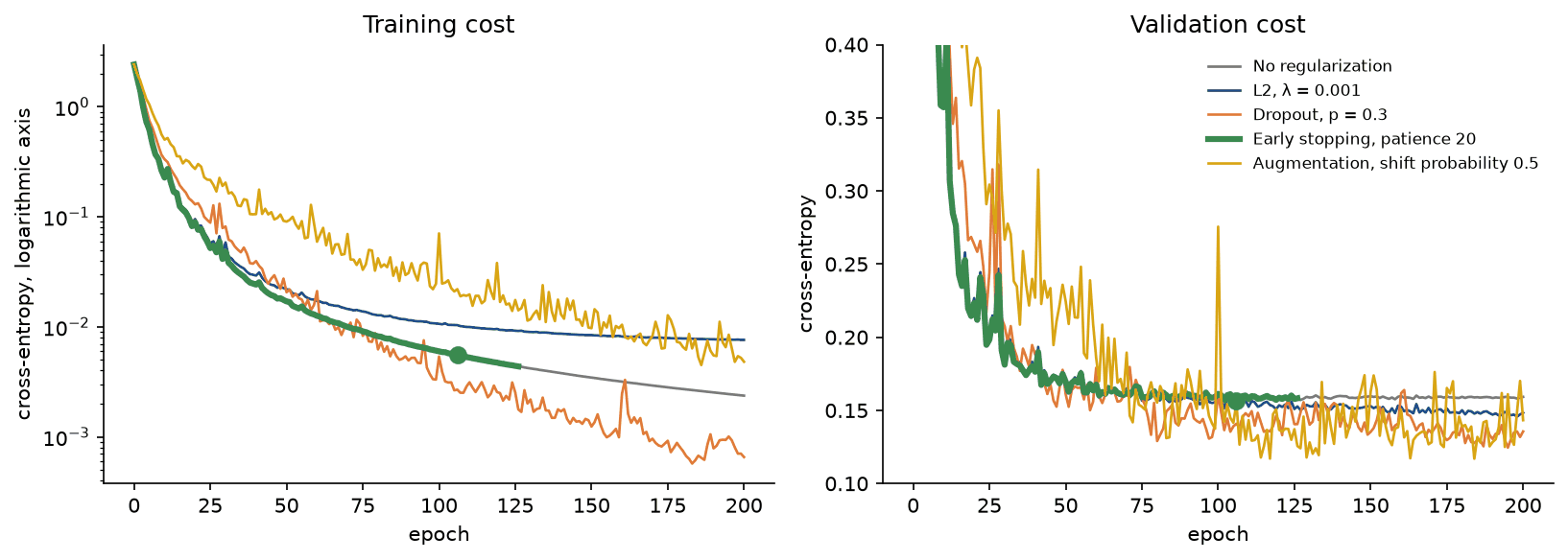
Every method fits the 200 training images perfectly; the differences are in how the network behaves on the other 1,597. The unregularized network's validation cost reaches its lowest point, 0.1566, at epoch 106 and then creeps up to 0.1592 while its training cost keeps falling, the overfitting pattern of the curve in milder form. L2, dropout and augmentation lower the test cost by 13 to 26 per cent and raise the test accuracy by 0.3 to 0.9 points. Early stopping trains for 126 epochs instead of 200, but on this problem the unregularized network overfits so slowly that stopping early buys little.

One split is one draw, so the project repeats the whole procedure, the choice of strengths included, on two further random splits and initializations. The test accuracies on splits 0, 1 and 2 are:

• No regularization: 0.9290, 0.9173 and 0.9457, mean 0.9307.
• L2: 0.9323, 0.9231 and 0.9457, mean 0.9337.
• Dropout: 0.9382, 0.9340 and 0.9449, mean 0.9390.
• Early stopping: 0.9290, 0.9173 and 0.9432, mean 0.9298.
• Augmentation: 0.9382, 0.9240 and 0.9507, mean 0.9376.

Every regularizer lowers the test cost on every split, from a mean of 0.2354 without regularization to 0.2080 with L2, 0.2007 with dropout, 0.2245 with early stopping and 0.1948 with augmentation. Accuracy tells a noisier story. L2 and augmentation match or beat the unregularized network on every split, dropout beats it on two of three, and early stopping never does. On split 2 the validation set preferred p = 0.5 to p = 0.3 by a validation cost difference of 0.0003, a coin toss, and dropout ended 0.08 points below the baseline. The spread between splits without regularization, 2.84 points, is larger than the gain of any single method, 0.83 points at best on average. On digits the honest summary is that regularization helps modestly and consistently, and that with 200 examples a single split cannot rank close methods; the comparison holds because it repeats.

L1 against L2 on the weights

Trained with the same settings, an L2 penalty of 0.003 and an L1 penalty of 0.0003 end up with almost the same validation cost (0.1533 and 0.1525, against 0.1592 without a penalty) and almost the same total absolute weight (1912 and 1917, against 3111). Their weights look very different. L2 makes the whole distribution narrower and keeps its bell shape. L1 produces a tall spike at zero with heavier tails: 31.1 % of the weights end within 0.001 of zero, against 0.5 % without a penalty. With the subgradient step not one of them is exactly zero, because they keep jumping across zero; with the proximal step 20.2 % of the weights are exactly zero, at the same validation accuracy, 0.9450.

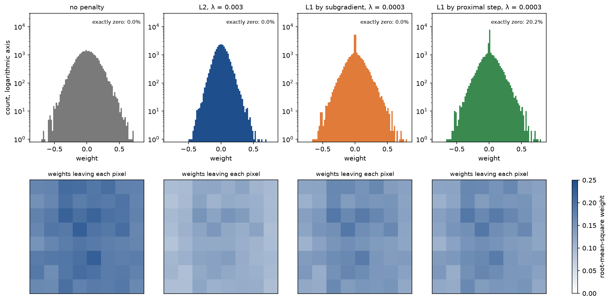
The maps underneath show the root-mean-square size of the first-layer weights leaving each pixel. Seven border pixels are zero in every training image. By B4 their weights never receive a data gradient, so without a penalty they keep their random initial size, 0.1649. Both penalties shrink them, to 0.0905 under L2 and 0.1208 under L1 after 200 epochs, so a network that has never seen a pixel light up reacts less to noise in it at test time.

Weight decay in Adam

The left panel below follows a weight with no data gradient. Under Adam with an L2 penalty it reaches 0.1098 after 100 steps from 0.2 whether λ is 0.001 or 0.1; the two paths differ by at most 6 × 10⁻⁶ over 2,000 steps, the remnant of the constant in the denominator, and both fall below 0.001 after about 500 steps. Under AdamW the same weight decays geometrically, to 0.1637 after 2,000 steps for λ = 0.1 and to 0.0270 for λ = 1, exactly 0.2 (1 - 10⁻³ λ) to the power 2,000.

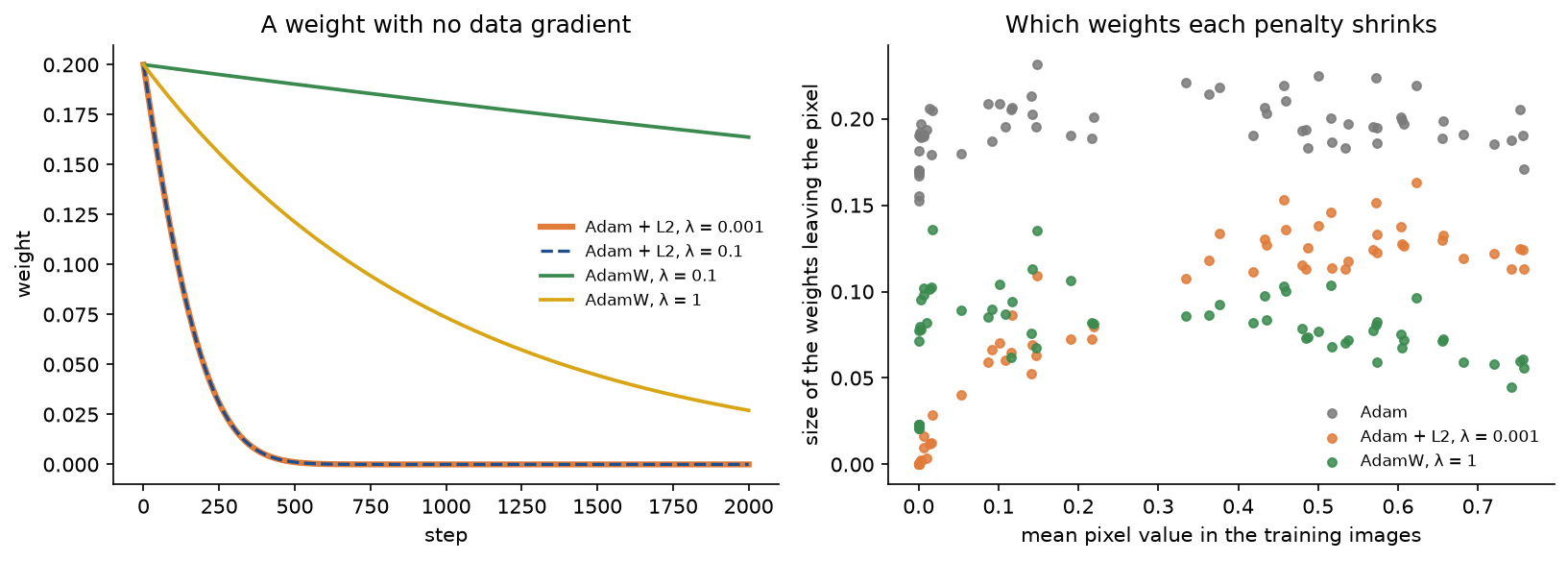
On the digits with learning rate 0.001, the right panel shows which weights each method shrinks. Relative to their initial size, Adam with an L2 penalty of λ = 0.001 shrinks the weights of dim pixels, with a mean value below 0.05, to 2.9 % and those of bright pixels, above 0.3, only to 71.1 %; AdamW with λ = 1 shrinks both by a similar factor, to 37.8 % and 42.8 %. Coupled L2 inside Adam is a strong penalty on the weights the data barely use and a weak one on the weights that matter; decoupled decay is uniform. In this short run neither improved on plain Adam (validation cost 0.1138 for Adam, 0.1303 with L2 and 0.1469 with AdamW at these strengths); the point is what each one does, and on longer training of larger models the decoupled form is the one whose strength can be tuned independently of the learning rate.

Augmentation, input noise and label smoothing

The same network and data, each change against the unregularized run with the same initial weights and batches, measured on the validation set after 200 epochs. Confidence is the mean probability the network gives its own prediction:

• No change: validation cost 0.1592, accuracy 0.9550, confidence 0.9582.
• Shifting every image by up to one pixel: 0.1848, 0.9375 and 0.9477.
• Shifting half the images: 0.1433, 0.9500 and 0.9553.
• Pixel noise with standard deviation 0.1: 0.1353, 0.9625 and 0.9666.
• Label smoothing with ε = 0.1: 0.2927, 0.9700 and 0.7919.

Augmentation has to match the data. On 8 by 8 images a one-pixel shift moves the digit by an eighth of its width; shifting every image in every epoch hurts, while shifting half of them lowers the validation cost and, in the project, the test cost. Pixel noise improves both cost and accuracy. Label smoothing gives the best accuracy but a higher cost, because the cost here is measured against hard labels while the network has been taught never to be more than 91 % sure; its mean confidence drops from 0.9582 to 0.7919. For linear regression examples/noise_and_augmentation.py confirms the identity between input noise and L2 numerically: least squares on 4,000 noisy copies of 30 examples with σ = 0.5 gives (0.8029, -1.4358, 0.4261), against (0.8011, -1.4376, 0.4267) from ridge regression with λ = σ² = 0.25 and (1.0039, -1.9987, 0.4878) without a penalty.

Augmenting before the split inflates the score. With 300 images and four augmented copies of each, a random split of the 1,500 rows leaves 93 to 94 % of the test rows with a sibling in training, and the network scores 0.9893 with pixel-noise copies and 0.8613 with shifted copies; splitting the originals first gives 0.8613 and 0.7813 on test sets built the same way.

The same in PyTorch

The NumPy implementation agrees with PyTorch everywhere the two can be compared, in double precision:

• Gradients through nn.Dropout on a batch of 20 digits, fed the masks PyTorch drew, differ by at most 1.7 × 10⁻¹⁶.
• The L2 run with SGD(weight_decay=0.001) follows ours to within 4.4 × 10⁻¹⁶ in validation cost over 200 epochs.
• Adam(weight_decay=0.001) follows adam_step(l2=0.001) to within 1.8 × 10⁻¹³, and AdamW(weight_decay=1) follows adam_step(weight_decay=1) to within 4.4 × 10⁻¹⁶.
• CrossEntropyLoss(label_smoothing=0.1) and smooth_labels give the same cost to ten decimals.

torch.nn.Dropout(p) takes the drop probability, multiplies survivors by 1/(1 - p) in training mode and is the identity after model.eval(). A dropout network trained with nn.Dropout, which draws its own masks, cannot match the NumPy run step for step but lands in the same place: validation cost 0.1368 and accuracy 0.9650 against 0.1356 and 0.9550. In PyTorch code the regularizers look like this:

model = torch.nn.Sequential(
    torch.nn.Linear(64, 128),
    torch.nn.ReLU(),
    torch.nn.Dropout(0.3),
    torch.nn.Linear(128, 128),
    torch.nn.ReLU(),
    torch.nn.Dropout(0.3),
    torch.nn.Linear(128, 10),
)
decay = [p for name, p in model.named_parameters() if name.endswith("weight")]
no_decay = [p for name, p in model.named_parameters() if name.endswith("bias")]
groups = [{"params": decay, "weight_decay": 0.05}, {"params": no_decay, "weight_decay": 0.0}]
optimizer = torch.optim.AdamW(groups, lr=1e-3)
criterion = torch.nn.CrossEntropyLoss(label_smoothing=0.1)

Call model.train() before each training epoch, and model.eval() together with torch.no_grad() for validation and testing. An L1 penalty is added to the loss by hand, loss + lam * sum(p.abs().sum() for p in decay), and autograd then supplies λ sgn w, as tests/test_comparisons.py checks. Early stopping is a loop that keeps copy.deepcopy(model.state_dict()) of the best epoch. Batch normalization shows the same two modes as dropout: in examples/compare_with_pytorch.py one example passed through a BatchNorm1d layer in training mode with three different sets of companions comes out as three different vectors, and in evaluation mode as one fixed vector.

When to use which

• More data first. Real data beats every regularizer, and label-preserving augmentation is the next best thing because it encodes knowledge of the task. Training image classifiers goes further with images.
• Always monitor a validation set and keep the best network. Early stopping is nearly free and protects against training too long, whatever else is used.
• Use decoupled weight decay with adaptive optimizers, AdamW rather than Adam with weight_decay, and exclude biases and normalization parameters; with SGD the two coincide. Typical strengths are 0.01 to 0.1 for long training; for short runs the per-step product ηλ is what matters.
• Dropout of 0.1 to 0.5 suits wide fully connected layers. It is less common in convolutional layers, where neighbouring activations are correlated and single-unit dropout is weak, and placed before a batch-normalization layer it changes the statistics that layer sees between training and evaluation.
• Use L1 when sparsity itself is the goal, with a proximal step or a final pruning of near-zero weights; for compressing networks, magnitude pruning is more common.
• Use label smoothing for classifiers with many classes when accuracy matters more than the probabilities themselves.
• Choose every strength on validation data, never on the test set, and repeat comparisons on several splits when the data are small.

Pitfalls

• Reusing one dropout mask. The mask must be redrawn for every mini-batch, and libraries draw an independent one for every example. Some descriptions drop a random half of the units and restore them only after a full epoch, or keep the same units dropped longer; that trains one thinned network at a time, and the units it drops learn nothing during that period, as tests/test_dropout.py shows. In examples/dropout_done_right.py, with the same network and batches, a fresh mask per example and mini-batch reaches validation accuracy 0.9675; one mask shared by each mini-batch 0.9450; one mask per epoch 0.9225; and one mask for the whole run 0.8650, because its never-trained units are switched back on at evaluation with their random initial weights.

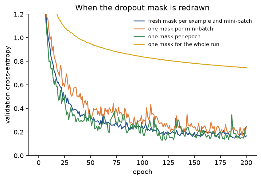
Only the correct policy gives a smooth, low curve; holding one mask for the whole run never recovers.

• Forgetting to scale. Training with masks but without dividing by q, and then evaluating the full network as it is, feeds every layer about 1/q times larger activations than it saw in training. In the worked example the subnetworks of example 1 average 0.74 while the unscaled evaluation output is 1.28. In examples/dropout_done_right.py the mean net input of the second hidden layer is 0.2567 with masks and 0.5119 in the full network, and the validation cost is 0.3473; scaling the weights by q for evaluation brings it to 0.2300, and inverted dropout reaches 0.1670. Use inverted dropout, or scale by q at evaluation, never neither.
• Leaving dropout on at evaluation. Without model.eval() every prediction is made by a random subnetwork. The network that scores 0.9675 deterministically scores 0.8200 on average over 20 masked passes, between 0.7875 and 0.8400, and 310 of the 400 validation images receive more than one label. Averaging 200 masked passes recovers 0.9675; that is Monte Carlo dropout, a deliberate choice, not a default. The same switch controls batch normalization.
• Drop probability or keep probability. torch.nn.Dropout(p) and most libraries take the probability of dropping; the original dropout paper wrote p for keeping. nn.Dropout(0.8) removes 80 % of the units and scales the survivors by 5, not 1.25, as examples/compare_with_pytorch.py prints.
• Decaying biases and normalization parameters. weight_decay in a PyTorch optimizer applies to every parameter it receives. With a zero data gradient, one SGD step with learning rate 0.1 and decay 0.5 shrinks a bias of 1 to 0.95. Put biases and normalization parameters in a parameter group with weight_decay=0.
• Calling an L2 penalty in Adam weight decay. Adam(weight_decay=λ) adds λθ to the gradient, which Adam then rescales per parameter: in the worked example it changes nothing on the first step, and for a weight with no data gradient the strength λ cancels entirely, as tests/test_optimizers.py checks. Use AdamW for weight decay, and remember that its per-step decay is the learning rate times λ.
• Comparing strengths across conventions. λ next to half the sum of squares, λ next to 1/(2n) times the sum of squares and AdamW's weight_decay are three different numbers for the same penalty, and scikit-learn's C is yet another, an inverse strength. Translate before reusing a published value, and re-tune λ when the training set size changes under a convention that includes n.
• Expecting exact zeros from L1 with plain gradient descent. The subgradient step oscillates across zero; on the digits it leaves 31.1 % of the weights within 0.001 of zero and none at zero. The proximal step gives exact zeros.
• Stopping early without restoring the best weights. When the patience runs out, the network is that many epochs past its best. On the first split of the project the best epoch is 106, training stops at 126, and the last network has validation cost 0.1582 against 0.1566 for the restored one. The validation set that chose the stopping epoch has been used for a choice, so report the test set.
• Augmenting before the split or augmenting the evaluation data. Near copies on both sides of the split inflate the score from 0.8613 to 0.9893 in examples/noise_and_augmentation.py. Random transformations applied to validation or test data make the score itself random. Check that each transformation preserves the label: shifting every 8 by 8 digit by a pixel in every epoch already hurts here.
• Checking gradients with dropout on. Each evaluation of the cost would use a different mask, so finite differences compare different functions: in examples/dropout_done_right.py the relative error is 1.0, the largest it can be. Hold the masks fixed, as gradient_check does, or switch dropout off, and include the penalty on both sides; with fixed masks and both penalties the check gives 4.4 × 10⁻¹⁰. Backpropagation covers gradient checking in general.
• Comparing a regularized cost with an unregularized one. The training cost reported during L2 training often includes λΩ. Compare models by the data cost or by the metric you care about, on validation data.

Further reading

• A. Krogh and J. A. Hertz, "A simple weight decay can improve generalization", Advances in Neural Information Processing Systems 4, 1992.
• R. Tibshirani, "Regression shrinkage and selection via the lasso", Journal of the Royal Statistical Society B 58(1), 267-288, 1996.
• I. Loshchilov and F. Hutter, "Decoupled weight decay regularization", International Conference on Learning Representations, 2019. The analysis behind AdamW.
• G. E. Hinton, N. Srivastava, A. Krizhevsky, I. Sutskever and R. R. Salakhutdinov, "Improving neural networks by preventing co-adaptation of feature detectors", arXiv:1207.0580, 2012.
• N. Srivastava, G. Hinton, A. Krizhevsky, I. Sutskever and R. Salakhutdinov, "Dropout: a simple way to prevent neural networks from overfitting", Journal of Machine Learning Research 15, 1929-1958, 2014.
• S. Wager, S. Wang and P. Liang, "Dropout training as adaptive regularization", Advances in Neural Information Processing Systems 26, 2013.
• Y. Gal and Z. Ghahramani, "Dropout as a Bayesian approximation: representing model uncertainty in deep learning", International Conference on Machine Learning, 2016. Monte Carlo dropout.
• L. Prechelt, "Early stopping, but when?", in Neural Networks: Tricks of the Trade, Springer, 1998.
• C. M. Bishop, "Training with noise is equivalent to Tikhonov regularization", Neural Computation 7(1), 108-116, 1995.
• C. Szegedy, V. Vanhoucke, S. Ioffe, J. Shlens and Z. Wojna, "Rethinking the Inception architecture for computer vision", Conference on Computer Vision and Pattern Recognition, 2016. Introduces label smoothing.
• R. Müller, S. Kornblith and G. Hinton, "When does label smoothing help?", Advances in Neural Information Processing Systems 32, 2019.
• S. Ioffe and C. Szegedy, "Batch normalization: accelerating deep network training by reducing internal covariate shift", International Conference on Machine Learning, 2015.
• P. Y. Simard, D. Steinkraus and J. C. Platt, "Best practices for convolutional neural networks applied to visual document analysis", International Conference on Document Analysis and Recognition, 2003. Augmentation for handwritten digits.
• C. Zhang, S. Bengio, M. Hardt, B. Recht and O. Vinyals, "Understanding deep learning requires rethinking generalization", International Conference on Learning Representations, 2017. Networks that fit random labels.
• I. Goodfellow, Y. Bengio and A. Courville, Deep Learning, chapter 7, 2016. Parameter penalties, the quadratic analysis of L2 and L1, early stopping as L2, and dropout as an ensemble.
• M. A. Nielsen, Neural Networks and Deep Learning, chapter 3, 2015.
• E. Alpaydin and C. Kaynak, Optical Recognition of Handwritten Digits, UCI Machine Learning Repository, 1998. The digits data.