Clustering

Clustering groups unlabelled points so that points in the same group resemble each other more than they resemble points in other groups. It is how customer segments, document topics, colour palettes, cell types and visual vocabularies are found, and it is one of the few tools that works before anyone has labelled anything. The catch is that "group" has no single definition: k-means looks for compact blobs around centres, hierarchical clustering builds a tree of nested groups, DBSCAN and mean shift look for dense regions, spectral clustering looks for weak cuts in a similarity graph and a Gaussian mixture fits a probability model. This page derives Lloyd's algorithm for k-means and proves that it converges, works it by hand on nine points together with k-means++ seeding, the silhouette and a MapReduce formulation, then works small examples of every other method and of the scores that judge a clustering. Each method is implemented from scratch in NumPy, compared on data sets where k-means fails, run on handwritten digits in a sample project and checked against scikit-learn and SciPy. Afterwards you will be able to run any of these algorithms on paper, choose the number of clusters with more than one criterion, predict which method suits which shape of data, and evaluate a clustering honestly. It builds on Probability and statistics for the mixture model and on Evaluation metrics for scoring.

To run the code in this topic, install the base group, and the ml group for the digits of the sample project and the comparisons with scikit-learn and SciPy.

Intuition

A clustering method needs two decisions before it can start: what makes two points similar, and what makes a set of points a group. Different answers give different families.

• Centroid methods. A cluster is the set of points nearest to a centre. k-means and mini-batch k-means belong here. They are good at compact, round clusters of similar size and scale to very large data; they struggle with elongated or nested shapes, unequal sizes and densities, and they need k.
• Hierarchical methods. A cluster is a branch of a tree of successive merges, with single, complete, average or Ward linkage deciding which clusters are closest. The tree shows structure at every scale, but memory grows with the square of the number of points and one bad early merge is never undone.
• Density methods. A cluster is a dense region bounded by sparse space. DBSCAN and mean shift find arbitrary shapes and flag outliers without being told k, but they struggle with clusters of different density, with high dimensions, and with their scale parameter.
• Graph methods. A cluster is a set of nodes with few edges to the rest of a similarity graph. Spectral clustering handles non-convex shapes such as rings and moons, at the price of choosing the graph and an eigen-decomposition whose cost grows with the cube of the number of points.
• Model-based methods. A cluster is a component of a probability distribution. A Gaussian mixture fitted by expectation-maximization gives elliptical clusters, soft membership and likelihood-based model choice, but assumes Gaussian shapes and can collapse a component onto a single point.

What clustering is not:

• Not classification. There are no labels to learn from and cluster numbers carry no meaning: clusters 0 and 1 might as well be called 1 and 0. Any evaluation against known classes must be invariant to renaming.
• Not a discovery of the true classes. A clustering answers the question its similarity and objective ask. Handwritten digits clustered by pixel distance put many nines with threes because the pixels agree, as the sample project shows. Kleinberg proved that no clustering function can satisfy three natural requirements at once (invariance to the scale of distances, the ability to produce any partition, and consistency when within-cluster distances shrink), so every method gives one of them up.
• Not evidence that groups exist. Every method here returns clusters for uniform noise. Whether the structure is real has to be tested, for example with the gap statistic below.
• Not invariant to units. Distances change when one feature is recorded in grams instead of kilograms, and so do the clusters.

k-means is the workhorse. Given k centres, every point joins its nearest centre; every centre then moves to the mean of its points; repeat until nothing changes. Both steps lower the same objective, so the loop must stop, but where it stops depends on where it started.

The blue cycle is Lloyd's algorithm. The two amber boxes are the decisions taken outside it, how many clusters and where to start, and the dashed orange arrow is the remedy for bad starts: run again from other seeds and keep the best run.

How it works

Notation

The data are n points x1 to xn with d features each, stored one per row. For a clustering into k clusters:

• d(x, y) is the Euclidean distance and the double bars ‖·‖ the Euclidean norm.
• C1 to Ck are the clusters, a partition of the points, with sizes n1 to nk; c(i) is the cluster of point i.
• μ is the centre of a cluster, x̄ the mean of a set of points, and J the k-means objective, also called inertia or the within-cluster sum of squares.
• During seeding, D(x) is the distance from x to the nearest centre chosen so far.
• For graphs, W holds the similarities w between pairs of points, g the degree of each node (the sum of its row of W), G the diagonal matrix of degrees and L the graph Laplacian.
• ε and m are DBSCAN's radius and minimum number of points, h is the bandwidth of a kernel, and π, Σ and γ are the weight, covariance and responsibility of a mixture component.

The formula images write indices as subscripts; the text writes them plainly, for example μ of cluster j or the centres m1, m2 and m3 of the worked example.

The k-means objective

k-means chooses a partition and centres that minimize the sum of squared distances from every point to its centre:

One identity carries most of the theory. Take any set C of points and any vector m, write x − m as (x − x̄) + (x̄ − m) and expand the square:

The cross term in the first line vanishes because the deviations from the mean sum to zero, which gives the second line. Its last term is never negative and is zero only at m equal to the mean, so the mean is the unique point that minimizes the sum of squared distances to a set. Applying the identity once for every point y of C as m and adding gives a second form without any centre:

So the objective also measures how far apart the points of each cluster are from one another.

Lloyd's algorithm and why it converges

Lloyd's algorithm alternates two steps, each of which minimizes J over one set of variables with the other held fixed:

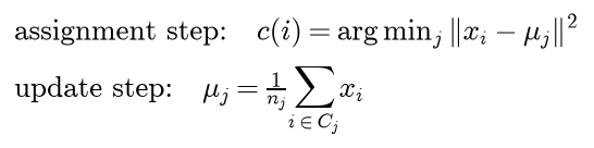
With the centres fixed, each term of J depends on one c(i) only, so choosing every term's minimum minimizes the sum. With the partition fixed, the identity says that the mean minimizes each cluster's contribution. A cluster that has lost all its points has no mean; implementations either keep its old centre or move it to a point far from its current centre, as ours and scikit-learn's do. The algorithm stops when an assignment step changes no label.

Convergence follows in three sentences. Neither step can raise J, and J is never negative. After every update step J is a function of the partition alone, because the centres are its means; breaking ties in favour of a point's current cluster, a point changes cluster only if that strictly lowers its distance, so J strictly decreases whenever the partition changes. A partition can therefore never be visited twice, and there are at most k to the power n of them, so the algorithm stops after finitely many iterations.

What it stops at is a fixed point: every point is nearest to the mean of its own cluster and no single step improves J. That is a local minimum in the partition sense, not the global one. Finding the global minimum is NP-hard even for k = 2 in general dimension and for general k in the plane. In practice Lloyd's algorithm needs few iterations, although point sets exist that force exponentially many. One iteration costs on the order of n k d operations for the distances.

The assignment step also fixes the shape of the clusters. A point is closer to the centre μa than to μb exactly when a linear inequality holds:

Every boundary is therefore a piece of the perpendicular bisector of two centres, and every cluster is a convex polyhedron (a Voronoi cell, a convex polygon in the plane), whatever the size, spread or shape of the cluster. Three failures follow directly:

• Unequal sizes. The boundary sits halfway between the centres, so a large loose cluster that extends past the bisector loses its edge to a small neighbour; and because J is dominated by the spread of the large cluster, splitting it in two can lower J more than separating the small cluster does.
• Unequal densities. Points on the fringe of a wide cluster that lie near a tight cluster's centre are given to the tight cluster.
• Non-convex shapes. Rings, moons and spirals are not unions of convex cells around one centre each.

Bad local minima and k-means++

A start with two centres inside one natural group and one centre between two others can be a fixed point that Lloyd's algorithm cannot leave: each step is optimal given the other, yet the whole is poor. Restarting from several seeds and keeping the lowest J helps; if one run ends badly with probability p, all of r independent runs do with probability p to the power r. Better seeds help more.

k-means++ chooses the first centre uniformly at random from the data, and every further centre at random with probability proportional to the squared distance to the nearest centre already chosen:

Points far from every current centre are likely; a point that is already a centre has D = 0 and cannot be drawn again. The square matters: D(x) squared is exactly what point x would contribute to J if seeding stopped now, so the rule samples points in proportion to their current cost. Arthur and Vassilvitskii proved for this rule that the seeds alone, before any Lloyd iteration, are within a logarithmic factor of the optimum J* in expectation:

The greedy variant used by scikit-learn draws 2 + ⌊ln k⌋ candidates at each step and keeps the one that lowers the sum of D squared the most. k-means|| (scalable k-means++) replaces the k sequential passes by a few rounds that each sample many candidates in parallel and then reclusters the weighted candidates; it is the default in Spark.

Choosing k

The elbow. Let J(k) be the optimal objective with k centres. Adding a centre at a data point that is not yet a centre leaves every point at most as far from its nearest centre as before, so J(k + 1) ≤ J(k), and J(n) = 0. The curve always falls; the elbow heuristic looks for the k after which it falls much more slowly. The elbow is often not sharp, and reading it is a judgement.

The silhouette. For point i in cluster C with more than one member, let a(i) be its mean distance to the other points of its own cluster and b(i) its mean distance to the points of the nearest other cluster:

s(i) lies between -1 and 1: near 1 when the point is much closer to its own cluster than to any other, near 0 on a boundary, negative when it would fit better elsewhere. A point alone in its cluster gets s(i) = 0 by convention. The silhouette of a clustering is the mean of s(i) over all n points, and the k with the largest mean silhouette is a candidate. It uses plain distances and needs at least two clusters and at most n − 1.

The gap statistic. Write W for the optimal within-cluster sum of squares with k clusters. On data without structure log W still falls as k grows, so its fall must be compared with the fall on data that has no clusters. Draw B reference data sets uniformly from the bounding box of the data (or from a box aligned with its principal axes), cluster each one, and compare:

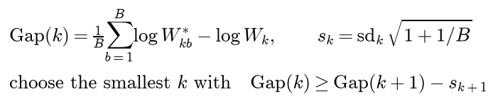
Because the reference has no clusters, the rule can answer k = 1, which no criterion built on the data alone can.

Hierarchical agglomerative clustering

Start with every point in a cluster of its own. Repeatedly merge the two closest clusters and record the distance at which they merged, until one cluster remains. The n − 1 merges form a binary tree, the dendrogram, in which the height of each internal node is its merge distance, and cutting the tree after n − k merges gives a partition into k clusters. What "closest clusters" means is the linkage:

Each linkage has a character:

• Single linkage follows long chains and thin curved clusters, and a single bridge of noise points merges two clusters.
• Complete linkage gives compact clusters of similar diameter and is sensitive to outliers.
• Average linkage is a compromise between the two.
• Ward linkage gives compact clusters of similar size, like k-means.

Ward linkage merges the pair whose union raises the k-means objective least. Apply the identity to A and to B with the mean of the union as m. The mean of the union lies on the segment between the two means, which gives the first line below, and substituting it gives the increase:

The Ward height is the square root of twice this increase, the convention of SciPy and scikit-learn, chosen so that two single points merge at their Euclidean distance.

After A and B merge, the distance from the new cluster to any other cluster C follows from the old distances alone, by the Lance-Williams formula. Its second line is the Ward case, written for squared distances:

Single linkage takes both α equal to one half, β = 0 and γ = -1/2, which is the minimum; complete linkage is the same with γ = +1/2, which is the maximum; average linkage weights the two old distances by the sizes of A and B with β = γ = 0. So the algorithm needs only the matrix of pairwise distances and memory for n squared numbers.

These four linkages never merge below a previous merge, so the heights increase up the tree. The cophenetic distance between two points is the height at which they first share a cluster; it satisfies the strong triangle inequality, so the distance from x to z is at most the larger of the distances from x to y and from y to z. Centroid and median linkage can produce inversions, merges lower than an earlier one, and are best avoided. Single linkage is the minimum spanning tree in disguise: Kruskal's algorithm adds the shortest edges in the same order as single linkage merges.

DBSCAN

DBSCAN defines clusters as regions where points are packed densely. The ε-neighbourhood of a point contains the point itself:

A point y is directly density-reachable from x if x is a core point and y lies in its neighbourhood, and density-reachable if a chain of such steps leads from x to y. A cluster is the set of all points density-reachable from one core point; a non-core point in a cluster is a border point, and a point in no cluster is noise. Two core points that reach each other belong to the same cluster, so the clusters of core points are well defined: they are the connected components of the graph that joins core points within ε. A border point within ε of core points from two clusters belongs to both by the definition, and an implementation must pick one, normally the cluster that reaches it first. With a spatial index the neighbourhood queries are cheap in low dimensions; brute force costs on the order of n squared.

A point is a core point exactly when its (m − 1)-th nearest other point lies within ε. Plotting these distances for all points in increasing order gives the k-distance plot, where dense regions form a flat part and noise a steep tail; ε is read near the knee.

Mean shift

Mean shift finds the modes, the local maxima, of a kernel density estimate. With a radially symmetric kernel whose profile κ is decreasing, the density estimate and its gradient are:

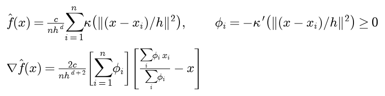
The last bracket of the gradient is the mean-shift vector: the weighted mean of the points minus the current position. It points along the gradient, and its length is the gradient divided by the sum of the weights, itself a density estimate, so steps are long in sparse regions and short near a mode. Mean shift moves to the weighted mean until the move is negligible:

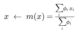
For the Gaussian profile the weights are again Gaussian. For the Epanechnikov profile κ(r) = 1 − r on r ≤ 1 the weights are 1 inside the window of radius h and 0 outside, so m(x) is simply the mean of the points within h: the flat kernel of scikit-learn's MeanShift. For these convex profiles the density increases at every step and the sequence converges (Comaniciu and Meer).

To cluster, start a trajectory at every point, collect the modes, keep each mode only if no stronger mode closer than h has been kept, and give every point to its nearest kept mode. The number of clusters follows from h; nobody chooses k. Each iteration of each trajectory touches every point, so the method is quadratic, and in high dimension a fixed window either holds almost nothing or almost everything.

Spectral clustering

Spectral clustering treats the points as nodes of a weighted graph and looks for a partition that cuts few, weak edges. Typical graphs are the Gaussian affinity and the symmetric nearest-neighbour graph, in which the weight is 1 when each of two points is among the other's nearest neighbours and 1/2 when only one of them is, scikit-learn's convention.

The Laplacian has a quadratic form that measures how much a vector f changes across edges. Splitting the degree term into two halves and using the symmetry of W gives:

So L is positive semidefinite and L times the all-ones vector is zero. Moreover the form is zero exactly when f is constant on every connected component, so the number of zero eigenvalues equals the number of connected components, and the indicator vectors of the components span their eigenspace. A graph made of k separate clusters is clustered by its k lowest eigenvectors.

When the clusters are joined by a few weak edges, the eigenvectors are close to indicators, and the second one solves a relaxed cut problem. For a split into A and its complement Ā, the RatioCut penalizes cutting off tiny pieces:

Choose a vector with one value on A and another on the complement as in the first line below. Only edges across the cut contribute to the quadratic form, each with the same squared difference, and the two values are chosen so that the result is n times the RatioCut while the vector is orthogonal to the all-ones vector and has squared length n:

Minimizing the RatioCut is therefore minimizing the Rayleigh quotient over two-valued vectors orthogonal to the ones vector, a combinatorial problem. Dropping the two-valued requirement leaves the minimum over all such vectors, which is the second smallest eigenvalue λ2 of L, attained by its eigenvector, the Fiedler vector. Hence λ2 is a lower bound for every RatioCut, and the signs of the Fiedler vector give an approximate best cut. For k clusters, the rows of the matrix of the first k eigenvectors embed the points in k dimensions and k-means clusters the embedding.

Measuring cluster size by volume, the sum of the degrees, instead of by count gives the normalized cut:

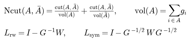
The same argument with the volume in place of the count leads to the eigenvectors of the random-walk Laplacian, whose second eigenvalue bounds the normalized cut from below. They are computed from the eigenvectors v of the symmetric Laplacian as G to the power -1/2 times v. Shi and Malik cluster these vectors; Ng, Jordan and Weiss cluster the v after scaling every row to unit length. scikit-learn's SpectralClustering uses the random-walk vectors without row scaling, which is also our default.

Concentric rings show why this works where k-means cannot. With a narrow Gaussian kernel a point's large weights go to its neighbours along its own ring, while every weight across the gap between the rings is tiny, so the graph is nearly two separate components. The first two eigenvectors are then nearly constant on each ring, the embedding collapses each ring to almost a single point, and k-means in the embedding separates them. With a wide kernel every point is similar to every other, the graph has no weak cut that follows the rings, and the relaxed cut becomes a straight line through both rings, the k-means answer.

Gaussian mixtures and EM

A Gaussian mixture models the data as drawn from k normal distributions with weights π that sum to 1:

The log of a sum has no closed-form maximizer, but the expectation-maximization algorithm (EM) climbs it by alternating two closed-form steps:

The responsibility γ of component j for point i is the posterior probability that the point came from that component; the M step is the maximum-likelihood fit of each component with every point counted with weight γ.

The likelihood never decreases. For any probabilities q that sum to 1 over the components, Jensen's inequality for the concave logarithm gives a lower bound for each point, with equality when q equals the responsibilities. Call the sum of the right-hand sides over the points F(q, θ):

The E step makes the bound tight at the current parameters, and the M step maximizes it over the parameters, so the likelihood can only rise. A likelihood that falls between iterations is a bug.

k-means is the hard limit of a constrained mixture. Fix every covariance to σ squared times the identity and every weight to 1/k. The responsibilities become a softmax of minus the squared distances, soft k-means:

As σ squared tends to 0 the largest term dominates, γ tends to 1 for the nearest centre and 0 for the others, the E step becomes the assignment step and the M step for the means becomes the update step. A full mixture relaxes all three assumptions of k-means at once: clusters may be elliptical (their own Σ), of different sizes (their own π) and overlapping (soft responsibilities).

The likelihood is unbounded: a component whose mean sits on one point and whose variance shrinks has a density at that point that grows without limit. EM can walk into this degenerate solution, so implementations add a small ridge to every covariance (reg_covar, 10⁻⁶ by default in scikit-learn and here). The number of components can be chosen with the Bayesian information criterion, where p counts the free parameters:

The k with the smallest BIC wins: each extra component must buy enough likelihood to pay for its parameters, a penalty that grows with the log of n.

Evaluating a clustering

External measures compare a clustering V with known classes U. Both are summarized by the contingency table: the count of points that belong to class i and to cluster j, with row sums a and column sums b.

Pair counting. Of all pairs of points, some are together in both partitions, some together in the classes only, some in the clusters only and the rest apart in both. The Rand index is the share of pairs on which the two partitions agree. With many clusters most pairs are apart in both, so even random labels score high. The adjusted Rand index (ARI) subtracts the value expected when the clustering is drawn at random with the same cluster sizes and rescales:

It is 1 for identical partitions, about 0 for random ones and can be negative.

Information. Entropies and mutual information are computed from the same table:

The arithmetic mean in the NMI denominator is scikit-learn's default; the geometric mean, the minimum and the maximum are also used, so a reported NMI should say which. Purity is easy to read but reaches 1 when every point is its own cluster. All of these are invariant to renaming the clusters.

Internal measures use only the data. Besides the silhouette, the Davies-Bouldin index averages, over clusters, the worst ratio of within-cluster spread S (the mean distance of a cluster's points to its centre) to between-centre distance, and the Calinski-Harabasz index is the ratio of between-cluster to within-cluster scatter:

Lower is better for Davies-Bouldin and higher for Calinski-Harabasz. Like the silhouette, both reward compact, convex, well separated clusters, which is not the same as rewarding the right clusters.

k-means at scale

Mini-batch k-means draws b random points per step, assigns them to the nearest centres, and moves each centre j towards each of its new points with step size 1/N, where N counts all points the centre has received so far:

With this step size each centre is the running mean of every point ever given to it, so its moves shrink as evidence accumulates. A step costs on the order of b k d instead of n k d operations, and the result comes within a few per cent of Lloyd's objective at a fraction of the cost.

MapReduce. One Lloyd iteration is one job, with the current centres broadcast to every mapper:

Vector sums and counts can be added in any order and grouping, so the combiner is legal and cuts the records shuffled from n to at most k per map task. Partial means cannot: averaging them ignores how many points each split held. The driver runs one job per iteration until the centres stop moving, rereading the data every time, which is why in-memory engines such as Spark, which cache the points between iterations, suit iterative algorithms better than Hadoop. MapReduce treats combiners and the averaging trap in general.

Worked example

Every value below is computed in double precision. Values that are not exact are rounded to four decimals.

Nine points and Lloyd's algorithm

Nine points in three loose groups and k = 3: A (2, 3), B (3, 2), C (4, 4), D (8, 2), E (9, 2), F (10, 5), G (4, 7), H (4, 9) and I (7, 8). The groups A to C, D to F and G to I have means (3, 3), (9, 3) and (5, 8). Start from the worst kind of random start, all three centres in the same group: m1 = G = (4, 7), m2 = H = (4, 9) and m3 = I = (7, 8). Every squared distance in this run is an integer or a fraction with a small power of two in the denominator, so the arithmetic is exact.

Iteration 1, assignment step. The squared distances of A to I are:

• to m1 = (4, 7): 20, 26, 9, 41, 50, 40, 0, 4, 10;
• to m2 = (4, 9): 40, 50, 25, 65, 74, 52, 4, 0, 10;
• to m3 = (7, 8): 50, 52, 25, 37, 40, 18, 10, 10, 0.

So cluster 1 is {A, B, C, G}, cluster 2 is {H} and cluster 3 is {D, E, F, I}, and the objective with these centres is the sum of the smallest distances, 20 + 26 + 9 + 37 + 40 + 18 + 0 + 0 + 0 = 150.

Iteration 1, update step. m1 = ((2 + 3 + 4 + 4)/4, (3 + 2 + 4 + 7)/4) = (3.25, 4), m2 = (4, 9) and m3 = ((8 + 9 + 10 + 7)/4, (2 + 2 + 5 + 8)/4) = (8.5, 4.25). The objective falls to 46.5: cluster 1 contributes 2.5625 + 4.0625 + 0.5625 + 9.5625 = 16.75 and cluster 3 contributes 5.3125 + 5.3125 + 2.8125 + 16.3125 = 29.75.

Iteration 2, assignment step:

• to m1 = (3.25, 4): 2.5625, 4.0625, 0.5625, 26.5625, 37.0625, 46.5625, 9.5625, 25.5625, 30.0625;
• to m2 = (4, 9): 40, 50, 25, 65, 74, 52, 4, 0, 10;
• to m3 = (8.5, 4.25): 43.8125, 35.3125, 20.3125, 5.3125, 5.3125, 2.8125, 27.8125, 42.8125, 16.3125.

G and I move to m2. The objective with the old centres and the new clusters is 34.625.

Iteration 2, update step. The clusters are now the three groups, so the centres become their means (3, 3), (5, 8) and (9, 3), and the objective is 4 + 8 + 8 = 20: the first group contributes 1 + 1 + 2, the second 2 + 2 + 4 and the third 2 + 1 + 5.

Iteration 3. Every point is already nearest to its own group's mean (C, for example, is at 2, 17 and 26), no label changes and the algorithm stops after three iterations. The objective went 150, 46.5, 34.625, 20, 20, never up, as the convergence proof requires.

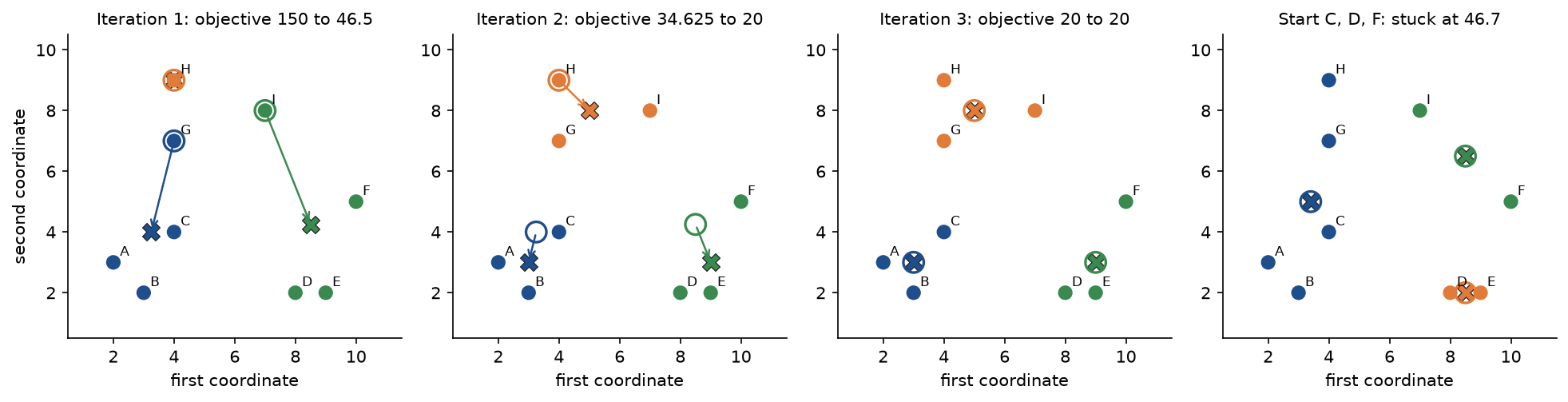
The first panel shows two centres moving out of the top group at once; by the third panel the centres sit on the group means and nothing moves. The last panel is the bad fixed point of the next subsection.

A bad local minimum

Start instead from C = (4, 4), D = (8, 2) and F = (10, 5). The first assignment step gives cluster 1 = {A, B, C, G, H} (squared distances to m1 of 5, 5, 0, 9 and 25), cluster 2 = {D, E} and cluster 3 = {F, I} (I is at 25, 37 and 18 from the three centres), with objective 63. The update gives m1 = (17/5, 25/5) = (3.4, 5), m2 = (8.5, 2) and m3 = (8.5, 6.5), and objective 37.2 + 0.5 + 9 = 46.7. In the second assignment step every point stays put (G, for example, is at 4.36 from m1 against 20.5 from m3), so the algorithm stops at 46.7, more than twice the optimum, with two groups merged and the third split.

Of the 84 ways to start from three distinct data points, 65 reach the optimum 20 and 19 end in bad fixed points: 46.7 (6 starts), 53 (7), 56 (2), 60.2667 (2), 71 (1) and 80 (1). A uniformly random start therefore fails with probability 19/84 = 0.2262, and the expected final objective is 27.7944.

k-means++ seeding

Suppose the first centre drawn is A. The squared distances D(x) squared of A to I to the nearest chosen centre, and the probabilities of being the second centre, are:

• D(x) squared: 0, 2, 5, 37, 50, 68, 20, 40, 50, with sum 272;
• probability: 0, 0.0074, 0.0184, 0.1360, 0.1838, 0.2500, 0.0735, 0.1471, 0.1838.

The second centre lands in A's own group with probability 7/272 = 0.0257, in the group D to F with 155/272 = 0.5699 and in the group G to I with 110/272 = 0.4044. The single most likely draw is F, with probability exactly 68/272 = 0.25. With A and F chosen, D(x) is the distance to the nearer of the two; for the point D, for example, D(x) squared = min(37, 13) = 13:

• D(x) squared: 0, 2, 5, 13, 10, 0, 20, 40, 18, with sum 108;
• probability: 0, 0.0185, 0.0463, 0.1204, 0.0926, 0, 0.1852, 0.3704, 0.1667.

The third centre now lands in the one group without a centre, G to I, with probability 78/108 = 0.7222. Enumerating every path the seeding can take, with the first centre uniform over all nine points, gives exact odds for k-means++ against three distinct points drawn uniformly:

• one centre in each group: 0.7150 with k-means++, 27/84 = 0.3214 uniformly;
• Lloyd's algorithm ends in a bad minimum: 0.1359 with k-means++, 19/84 = 0.2262 uniformly;
• expected final objective: 24.3649 with k-means++, 27.7944 uniformly.

k-means++ more than doubles the chance of one centre per group but does not guarantee it; on these nine points it still ends badly about once in seven runs. Ten restarts, each failing with probability 0.1359, all fail with probability 0.1359 to the power 10, about 2 × 10⁻⁹. A simulation of 20,000 draws of the second centre reproduces the first list of probabilities to within 0.0064.

Choosing k on the nine points

The optimal objective J*(k) for k = 1 to 6 is 126, 63.5, 20, 12.5, 6.5 and 3.5, and the mean silhouette of the optimal partition for k = 2 to 6 is 0.4158, 0.5470, 0.4967, 0.4347 and 0.3158. The objective drops by 62.5 and 43.5 for the first two added centres and by at most 7.5 afterwards: an elbow at k = 3, where the silhouette also peaks. The silhouette quantities of A to I in the three-cluster solution are:

• a: 1.8251, 1.8251, 2.2361, 2.3028, 2.0811, 3.3839, 2.5811, 2.5811, 3.1623;
• b: 5.9559, 6.2053, 4.3333, 5.1850, 6.1521, 5.9261, 4.1904, 6.1319, 5.5500;
• s: 0.6936, 0.7059, 0.4840, 0.5559, 0.6617, 0.4290, 0.3840, 0.5791, 0.4302.

For A, the distances to B and C are √2 and √5, so a(A) = (1.4142 + 2.2361)/2 = 1.8251. Its mean distance to the group G to I is (√20 + √40 + √50)/3 = (4.4721 + 6.3246 + 7.0711)/3 = 5.9559 and to the group D to F it is (√37 + √50 + √68)/3 = 7.1333; the nearer cluster gives b(A) = 5.9559, and s(A) = (5.9559 − 1.8251)/5.9559 = 0.6936. The lowest value belongs to G, which sits only 3 from C: b(G) = (√20 + √26 + 3)/3 = 4.1904 against a(G) = (2 + √10)/2 = 2.5811. The mean over the nine points is 0.5470.

One iteration as a MapReduce job

Store the points in three splits, {A, D, G}, {B, E, H} and {C, F, I}, and broadcast the starting centres G, H and I. The mappers emit the cluster of iteration 1's assignment step for every point, the combiners add vectors and counts within each split, and each reducer divides.

The reducer for m1 receives three partial sums and computes ((6 + 3 + 4)/4, (10 + 2 + 4)/4) = (3.25, 4), the one for m2 receives one and gives (4, 9), and the one for m3 receives three and gives (34/4, 17/4) = (8.5, 4.25): exactly iteration 1's update. Seven records cross the network instead of nine. Had the combiners sent partial means, (3, 5), (3, 2) and (4, 4) for m1, the reducer's unweighted average would be (3.3333, 3.6667), not (3.25, 4).

Hierarchical clustering of seven readings

The seven numbers 0, 4, 7, 13, 14, 23 and 25, with every linkage. The first three merges join the closest pairs, {13, 14} at 1, {23, 25} at 2 and {4, 7} at 3, and the fourth adds 0 to {4, 7} in every linkage, at height 4 (single, the nearer distance), 7 (complete, the farther one), (4 + 7)/2 = 5.5 (average) and √(2 · 1 · 2 / 3) · |0 − 5.5| = 6.3509 (Ward). The fifth merge decides where {13, 14} goes:

• Single linkage: 13 − 7 = 6 to the left group {0, 4, 7} against 23 − 14 = 9 to the right pair {23, 25}, so it goes left.
• Complete linkage: 14 − 0 = 14 to the left against 25 − 13 = 12 to the right, so it goes right.
• Average linkage: 59/6 = 9.8333 to the left, the mean of the six gaps 13, 9, 6, 14, 10 and 7, against 42/4 = 10.5 to the right, the mean of 10, 12, 9 and 11, so it goes left.
• Ward linkage: √(12/5) · (13.5 − 11/3) = 15.2337 to the left against √2 · (24 − 13.5) = 14.8492 to the right, so it goes right.

The full sequences of merge heights are 1, 2, 3, 4, 6, 9 for single linkage, 1, 2, 3, 7, 12, 25 for complete, 1, 2, 3, 5.5, 9.8333, 16.4 for average and 1, 2, 3, 6.3509, 14.8492, 27.9289 for Ward. All four agree on three clusters, {0, 4, 7}, {13, 14} and {23, 25}, and split two ways on two: single and average linkage give {0, 4, 7, 13, 14} and {23, 25}, complete and Ward give {0, 4, 7} and {13, 14, 23, 25}.

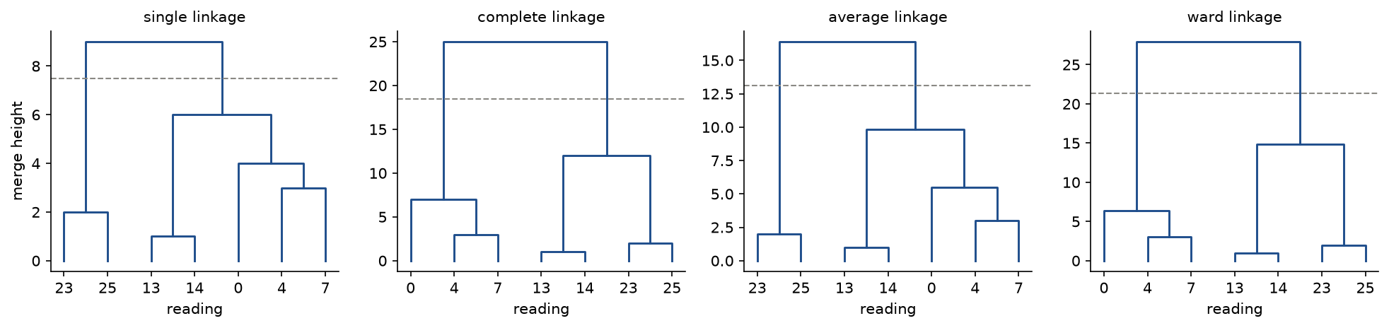
Single linkage looks only at the nearest gap (6 against 9) and complete only at the farthest; Ward compares means weighted by size, and the larger left group costs more to join. The dashed lines show the two answers for two clusters.

DBSCAN on a line

The nine numbers 1, 2, 3, 4.2, 5.5, 9, 10, 10.8 and 14 with ε = 1.5 and m = 3. The neighbourhoods, counting the point itself, hold 2, 3, 3, 3, 2, 2, 3, 2 and 1 points, so 2, 3, 4.2 and 10 are core points.

• Cluster 0: the core points 2, 3 and 4.2 reach one another in steps of at most 1.5; 1 and 5.5 join as border points but extend the cluster no further.
• Cluster 1: 10 is its only core point, and 9 and 10.8 join as border points.
• Noise: 14 has no neighbour.

The gap from 5.5 to 9 is wider than ε, so nothing connects the two clusters.

Mean shift on the same line

A flat kernel with h = 1.5; every point is a seed and moves to the mean of the points within 1.5 of its current position:

• From 1: the window holds {1, 2}, mean 1.5; from 1.5 it holds {1, 2, 3}, mean 2, a fixed point.
• From 2 nothing moves; from 3 the trajectory goes to 3.0667 and from 4.2 to 4.2333; from 5.5 the window holds {4.2, 5.5}, mean 4.85, and stays.
• From 9 the trajectory goes 9, 9.5, 9.9333; from 10 it goes to 9.9333; from 10.8 it goes 10.4, 9.9333.
• From 14 nothing moves.

Ranking the modes by the number of points in their window and keeping a mode only when no stronger kept mode lies within h keeps 9.9333, then 4.2333 (which absorbs 3.0667 and 4.85), then 2 (whose distance to 4.2333 is 2.2333), then 14: four clusters, {1, 2, 3}, {4.2, 5.5}, {9, 10, 10.8} and {14}. The bandwidth alone sets their number: 5 clusters at h = 1, 4 at 1.5, 3 at 2 and at 3, and 1 at 5. With h = 2 the result is DBSCAN's two clusters plus 14 as a cluster of its own; mean shift has no notion of noise.

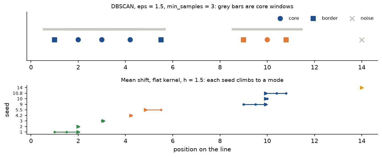
The top panel shows why 5.5 is a border point: it lies inside the window of 4.2 but its own window holds only two points. The bottom panel shows the seeds converging on four modes.

Spectral clustering of a small graph

Two triangles of weight-1 edges, nodes 1, 2, 3 and 4, 5, 6, joined by one edge of weight 0.5 between nodes 3 and 4.

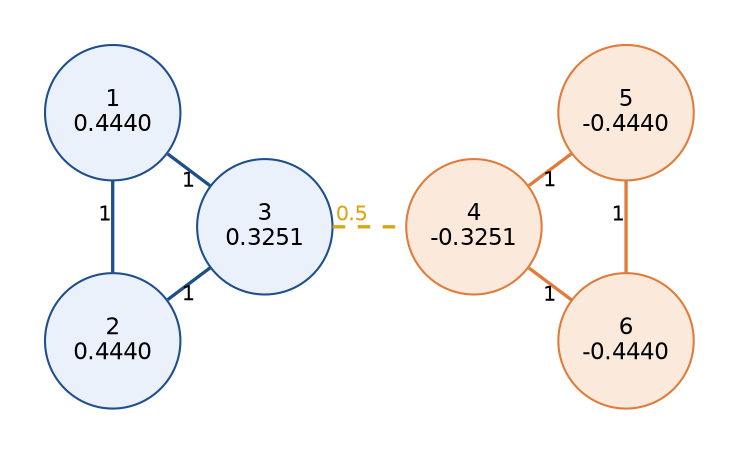
The degrees are 2, 2, 2.5, 2.5, 2 and 2. Row 1 of the Laplacian is (2, -1, -1, 0, 0, 0) and row 3 is (-1, -1, 2.5, -0.5, 0, 0); the rows of the second triangle mirror these. The graph is symmetric under swapping the triangles, so the Fiedler vector should be antisymmetric, f = (a, a, b, -b, -a, -a), and two rows of L f = λ f determine it:

Scaling to unit length, which requires a squared times (12 − 4√3) = 1, gives f = (0.4440, 0.4440, 0.3251, -0.3251, -0.4440, -0.4440), the numbers in the diagram. The full spectrum is 0, 0.2679, 3, 3, 3 and 3.7321, the last being the other root, 2 + √3. The signs of f cut the bridge and nothing else, and the bridge nodes 3 and 4 have the smallest entries in magnitude, as the least certain members. The RatioCut of that split is 0.5 · (1/3 + 1/3) = 0.3333, at least λ2 = 0.2679, as the relaxation predicts. The normalized cut of the same split is 0.5/6.5 + 0.5/6.5 = 0.1538, and the second eigenvalue of the random-walk Laplacian is 0.1272, again below it, with eigenvector (0.3046, 0.3046, 0.2271, -0.2271, -0.3046, -0.3046): the same cut.

One EM step

The six numbers 1, 2, 3, 6, 7 and 9 and a two-component mixture started with equal weights 1/2, means 2 and 6, and variances 2. With equal weights and variances the responsibility of the first component is a logistic function:

For the six points t is 6, 4, 2, -4, -6 and -10. For x = 3, for example, t = (9 − 1)/4 = 2 and 1/(1 + e⁻²) = 0.8808: the point is three times as close to 2 as to 6 but still gives 0.1192 of itself to the second component.

• Responsibilities of the first component: 0.9975, 0.9820, 0.8808, 0.0180, 0.0025, 0.0000, summing to 2.8808; the second component's sum to 3.1192.
• M step: weights (0.4801, 0.5199), means (1.9889, 7.1399), variances (0.7740, 2.3618).
• The log-likelihood rises from -14.5837 to -12.8519 in this one step.

The first mean is (0.9975 · 1 + 0.9820 · 2 + 0.8808 · 3 + 0.0180 · 6 + 0.0025 · 7 + 0.0000 · 9)/2.8808, which is 1.9888 from the rounded terms and 1.9889 at full precision. Run to convergence, EM settles at weights (0.4994, 0.5006), means (1.9988, 7.3280) and variances (0.6664, 1.5771), close to k-means's hard answer of means 2 and 7.3333 for the groups {1, 2, 3} and {6, 7, 9}.

Scoring a clustering against labels

Ten points in three classes, (0, 0, 0, 0, 1, 1, 1, 2, 2, 2), and a clustering (0, 0, 0, 1, 1, 1, 1, 2, 2, 0) that puts one point of class 0 with class 1 and one point of class 2 with class 0. With classes as rows and clusters as columns, the contingency table has rows (3, 1, 0), (0, 3, 0) and (1, 0, 2), row sums (4, 3, 3) and column sums (4, 4, 2).

Pairs together in both: 3 + 3 + 1 = 7. Together in the classes: 6 + 3 + 3 = 12; in the clusters: 6 + 6 + 1 = 13. Of the 45 pairs, 12 − 7 = 5 are together only in the classes, 13 − 7 = 6 only in the clusters and 45 − 7 − 5 − 6 = 27 apart in both, so the Rand index is (7 + 27)/45 = 0.7556. The expected count is E = 12 · 13 / 45 = 3.4667 and the maximum (12 + 13)/2 = 12.5, so

The mutual information is 0.6390, the entropies are 1.0889 and 1.0549 with mean 1.0719, and the NMI is 0.6390/1.0719 = 0.5962. Purity is (3 + 3 + 2)/10 = 0.8. Two misplaced points out of ten leave the Rand index near the top of its range but cut the ARI to 0.3911, which is the more honest summary.

Every number in this section is asserted by the tests: the Lloyd runs in tests/test_lloyd.py, the starts and seeding odds in tests/test_worked_example.py and tests/test_seeding.py, the silhouettes in tests/test_internal_indices.py, and the other methods in the test file of their module. examples/worked_example.py prints them all.

The code

The package clustering is plain NumPy, split into one module per idea. scikit-learn and SciPy are imported only inside the functions of datasets.py (for the digits), comparisons.py and library_trees.py, so everything else works without them.

• arrays.py holds the array types and the checks that every input is a matrix of points, one per row, or a vector of labels.
• distances.py computes squared and pairwise Euclidean distances, exactly for small inputs and by expanding the square for large ones.
• lloyd.py is the heart of the topic: assign_to_nearest, cluster_means, relocate_empty_clusters, kmeans_objective and lloyd, which records every iteration for small inputs.
• seeding.py holds random seeding and k-means++ with its greedy variant, and enumerates every k-means++ outcome with its exact probability.
• restarts.py runs k-means from several seeds and keeps the best run.
• minibatch.py and mapreduce.py hold the two versions at scale: mini-batch updates, and the mapper, combiner, reducer and driver of the MapReduce job.
• internal_indices.py computes the silhouette, Davies-Bouldin and Calinski-Harabasz; choosing_k.py adds the elbow, the two dispersion formulas and the gap statistic.
• hierarchical.py builds linkage trees with the Lance-Williams update in SciPy's format and cuts them; dendrograms.py reads them as trees: leaf order, drawing segments and cophenetic distances.
• density.py holds DBSCAN and the k-distance curve; mean_shift.py holds the kernel density, trajectories and mean-shift clustering.
• spectral.py builds affinities and Laplacians, the spectral embedding, spectral clustering, and the RatioCut and normalized cut.
• mixtures.py holds the E and M steps, EM, Gaussian mixtures and soft k-means responsibilities.
• metrics.py holds the contingency table, pair counts, Rand and adjusted Rand indices, entropy, mutual information, NMI and purity.
• worked_example.py builds the small data sets of this page and computes the exact odds of every start; trace.py prints Lloyd runs, seedings, silhouettes and merges in the order of this page.
• datasets.py generates blobs, rings and moons from a seed, names the data sets the examples share, and loads the digits.
• studies.py, scale_study.py and digit_study.py hold the experiments of the examples and the project, so the notebook and the tests can rerun them.
• pitfalls.py holds deliberately wrong computations for the Pitfalls section.
• comparisons.py and library_trees.py run scikit-learn and SciPy on the same inputs and report how far they are from ours.
• plotting.py and cluster_plots.py draw every figure in the handbook's colours and save it reproducibly.

Lloyd's loop in lloyd.py is the two steps of the proof plus the stopping rule; the full function also records each iteration:

for _ in range(max_iterations):
    labels, squared = assign_to_nearest(points, centers)
    if np.any(np.bincount(labels, minlength=k) == 0):
        labels = relocate_empty_clusters(labels, squared, k)
    updated = cluster_means(points, labels, k, centers)
    centers = updated
    if previous_labels is not None and np.array_equal(labels, previous_labels):
        converged = True
        break
    previous_labels = labels

Ties go to the lowest-numbered centre, as in NumPy's argmin and scikit-learn, and the iteration count follows scikit-learn's, so the confirming pass that changes nothing counts as an iteration. The agglomerative code keeps the full distance matrix and, for every cluster, its nearest other cluster; after a merge the Lance-Williams formula updates one row, and only the clusters whose nearest neighbour took part in the merge are rescanned, which takes under a second for the 1,797 digits.

The examples and the project import the package, so install the repository first as described in the main README. Each example demonstrates one idea and runs in seconds from the repository root:

• examples/worked_example.py prints every number of the worked examples in the order above and saves the Lloyd, dendrogram and line figures.
• examples/choosing_k_and_seeding.py scores four blobs with the elbow, the silhouette and the gap statistic, and compares 200 single runs from three seedings on a grid of 25 blobs.
• examples/method_comparison.py runs seven methods on five data sets built to break k-means, then studies spectral clustering on rings, DBSCAN on noisy moons, mean shift's bandwidth and a Gaussian mixture on stretched blobs.
• examples/kmeans_at_scale.py compares full Lloyd iterations, mini-batch k-means, the MapReduce formulation and scikit-learn on 300,000 points, in well under half a minute.
• examples/common_mistakes.py demonstrates every pitfall listed below that is not covered by another example.
• examples/compare_with_libraries.py runs each method next to scikit-learn or SciPy and prints how far apart they are.

python machine-learning/clustering/examples/worked_example.py
python machine-learning/clustering/examples/choosing_k_and_seeding.py
python machine-learning/clustering/examples/method_comparison.py
python machine-learning/clustering/examples/kmeans_at_scale.py
python machine-learning/clustering/examples/common_mistakes.py
python machine-learning/clustering/examples/compare_with_libraries.py

The sample project, project/digit_clustering.py, clusters the 1,797 handwritten digits that ship with scikit-learn, 8 by 8 images treated as points in 64 dimensions, as an analyst without labels would: four methods, a range of k, and the silhouette to choose k. Only afterwards are the labels used, to score the chosen clustering and to name each cluster by its majority digit.

Each method reuses what does not depend on k: Ward builds one tree and cuts it at every k, and spectral clustering computes one embedding and clusters its first k columns. Options such as --k-min, --k-max, --seed, --restarts, --neighbors and --reg-covar change the setup, and --figures sends the two PNGs to another folder so a custom run does not overwrite the ones shown here; the default run takes well under half a minute on one thread.

python machine-learning/clustering/project/digit_clustering.py
python machine-learning/clustering/project/digit_clustering.py --k-max 20 --neighbors 15

With the defaults the silhouette chooses k = 9 for k-means and for Ward linkage, k = 10 for spectral clustering and k = 12 for the Gaussian mixture. Against the digit labels:

• k-means at k = 9: silhouette 0.1894, ARI 0.5990, NMI 0.7238; at k = 10 it would have scored ARI 0.6649 and NMI 0.7421.
• Ward at k = 9: silhouette 0.1806, ARI 0.7470, NMI 0.8447; at k = 10, ARI 0.7940 and NMI 0.8682.
• Spectral clustering at k = 10: silhouette 0.1827, ARI 0.7565, NMI 0.8536.
• Gaussian mixture at k = 12: silhouette 0.1798, ARI 0.7228, NMI 0.7909; at k = 10, ARI 0.7062 and NMI 0.7749.

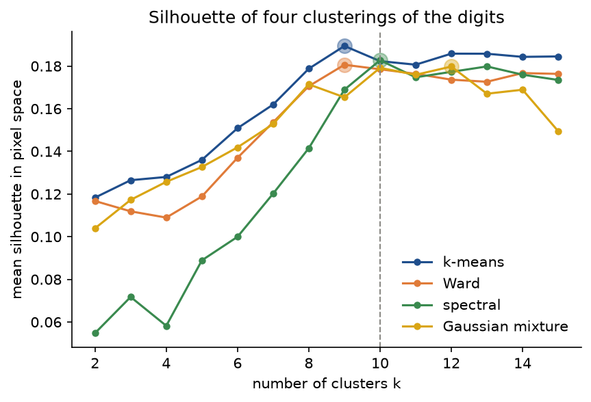
Silhouettes below 0.2 say that the digits are not compact, separated blobs in pixel space, and the flat curves from k = 9 onwards mean the choice of k is fragile: it lands within two of the ten classes for every method, but never by a wide margin.

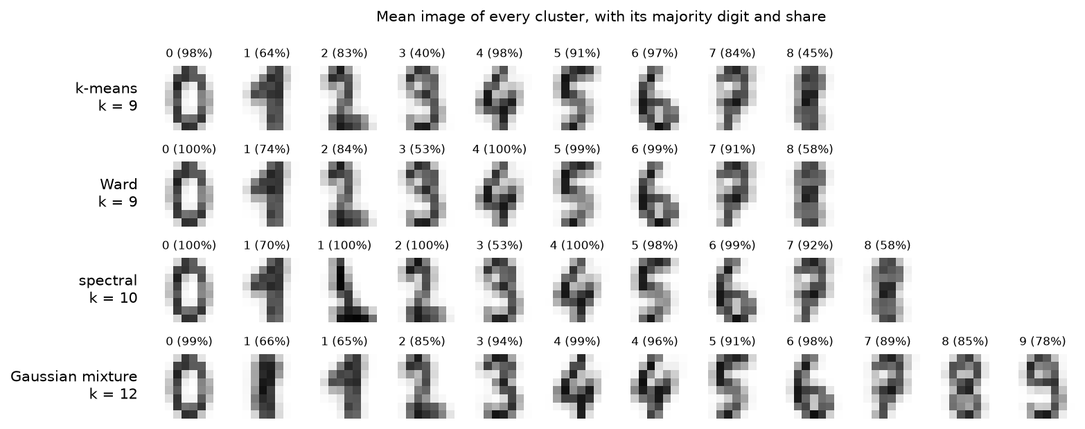
The prototypes show what the silhouette cannot. With nine clusters, k-means and Ward have no cluster for 9: the nines share a cluster with the threes (145 nines beside 164 threes in k-means' largest cluster), and about a hundred ones share one with the eights. Spectral clustering repeats both merges at k = 10 and spends its tenth cluster on ones with a foot. The Gaussian mixture separates the nines but splits ones and fours into two clusters each. All four methods agree that 0, 4 and 6 are easy and that 1, 3, 8 and 9 overlap in pixel space; clustering features from Dimensionality reduction instead of raw pixels often helps on data like these.

The notebook clustering.ipynb is a guided tour in the order of this page: the worked examples through the package and once more in a few lines of bare NumPy, the methods on shapes that break k-means, the pitfalls, k-means at scale on a smaller sample, the digits, and the comparisons with scikit-learn and SciPy. The tests in tests check the worked examples value by value, the mathematical properties above and the agreement with both libraries, and run in a few seconds:

python -m pytest machine-learning/clustering

Data: the synthetic sets are generated from fixed seeds by make_blobs, make_rings and make_moons, so nothing is downloaded and no licence is involved. The digits are the Optical Recognition of Handwritten Digits data of E. Alpaydin and C. Kaynak (1998) from the UCI Machine Learning Repository, available under the Creative Commons Attribution 4.0 licence; scikit-learn ships a copy of its test portion, 1,797 images of 8 by 8 pixels with intensities from 0 to 16, as sklearn.datasets.load_digits, so nothing is downloaded for them either.

In practice

Where k-means fails, and what works instead

Five data sets built to break k-means, clustered by seven of our implementations. k-means, the Gaussian mixture, Ward and single linkage and spectral clustering on a 10-nearest-neighbour graph were given the true number of clusters; DBSCAN's ε and m and mean shift's bandwidth were set per data set by looking at the results, which flatters those two. The adjusted Rand index against the true labels, in the order k-means, Gaussian mixture, Ward, single linkage, DBSCAN, mean shift and spectral, is:

• Unequal sizes (400 loose points beside 40 tight ones): 0.304, 0.967, 0.122, -0.004, 0.848, 0.689, 0.967.
• Unequal densities: 0.799, 0.948, 0.916, 0.000, 0.954, 0.812, 0.910.
• Stretched blobs: 0.567, 1.000, 0.627, 0.570, 0.990, 0.813, 0.993.
• Concentric rings: -0.002, 0.000, -0.002, 1.000, 0.995, 0.377, 1.000.
• Two moons: 0.224, 0.503, 0.705, 1.000, 1.000, 0.266, 1.000.

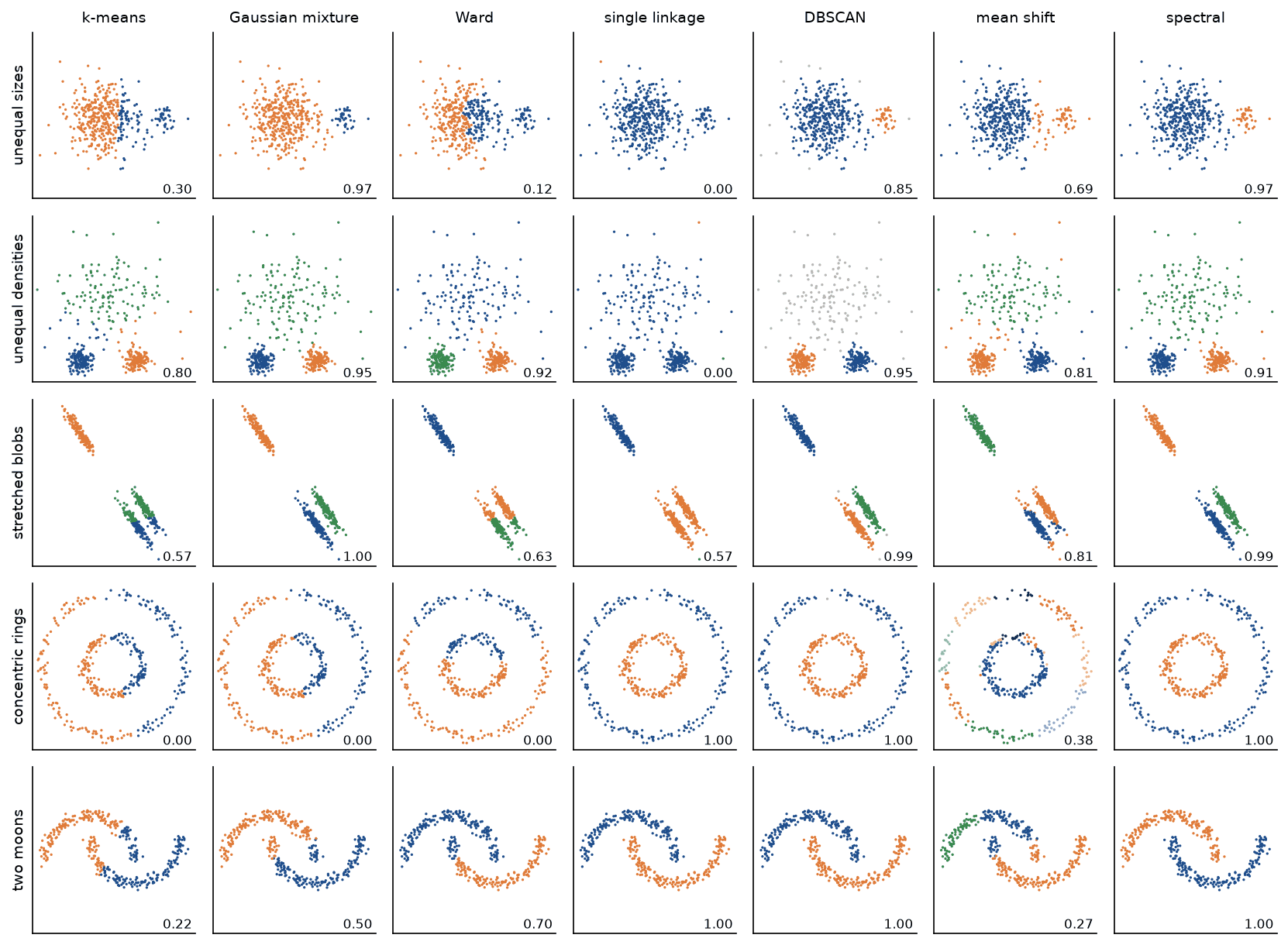
The pattern follows the mathematics. k-means and Ward, which minimize the same objective, cut the large cluster in two and slice the stretched blobs across their long axes. The Gaussian mixture fixes size, density and shape at once but, like k-means, cannot bend around rings or moons. Single linkage follows any thin connected shape and fails as soon as clusters touch or are blobs of noise-like points. DBSCAN handles shapes and noise, but its single ε cannot serve two densities: on the unequal-densities data its 0.954 comes from labelling the entire sparse cluster as noise, which the ARI happens to count as one more cluster. Spectral clustering on a neighbour graph is the most consistent of the seven here.

Choosing k

Four blobs, two of them close together, so that both k = 3 and k = 4 are defensible. For k = 1 to 9:

• objective: 7841.2, 4432.3, 1146.8, 632.1, 544.9, 480.4, 439.5, 405.3, 376.6;
• mean silhouette (from k = 2): 0.5077, 0.6890, 0.6445, 0.5547, 0.4618, 0.4604, 0.3565, 0.3367;
• gap statistic: 0.3315, 0.4136, 1.3004, 1.4535, 1.4205, 1.3347, 1.2038, 1.1939, 1.1374.

The elbow is clearest at k = 3, the silhouette peaks at k = 3, and the gap statistic chooses k = 4, because Gap(4) = 1.4535 is at least Gap(5) − s = 1.4205 − 0.0306, while Gap(3) = 1.3004 falls short of 1.4535 − 0.0278. The silhouette penalizes splitting two touching blobs because their points are close to each other's cluster; the gap statistic credits the extra drop in log W against noise. Both answers are reasonable, and the disagreement is information: there is structure at two scales.

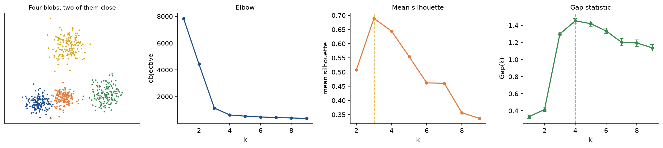
The elbow bends at 3 and flattens after 4, which is why reading it is a judgement; the dashed lines mark the two criteria's choices.

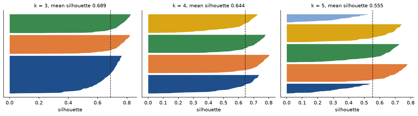
At k = 3 the two close blobs form one wide cluster; at k = 4 they become two clusters with slightly lower silhouettes; at k = 5 a real blob is split and two thin clusters with low values appear, the visual sign of too many clusters.

Random starts against k-means++

Single runs on 25 blobs in a 5 by 5 grid, 200 from each seeding:

• Three distinct random points: median objective 2.2215 times the best, worst 4.0286 times, 0.005 of the runs reach the best, 11.4 iterations on average.
• k-means++: median 1.7843, worst 2.7066, 0.065 of the runs reach the best, 8.9 iterations.
• Greedy k-means++ with 5 candidates per draw: median 1.0000, worst 1.8102, 0.645 of the runs reach the best, 4.9 iterations.

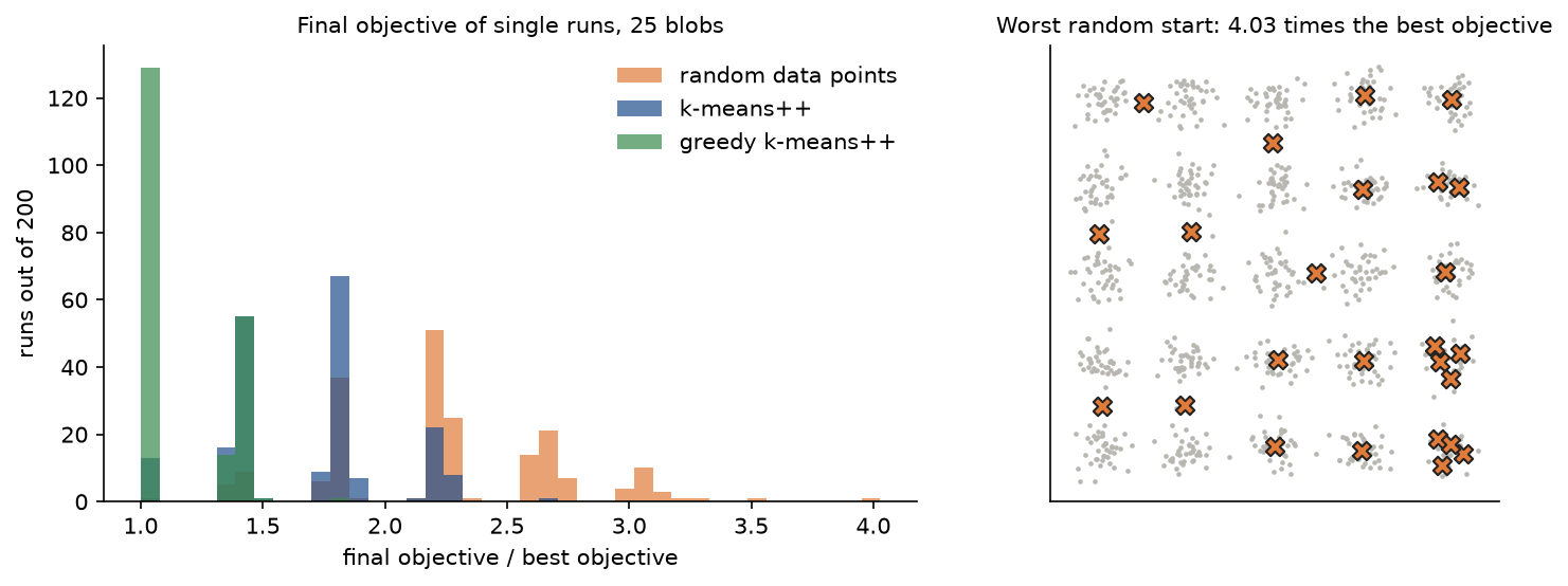
With many clusters a random start almost always leaves some blob with two centres and some pair of blobs sharing one, and Lloyd's algorithm cannot move a centre across the empty space between blobs; the right panel shows such a start. Plain k-means++ helps but still errs on a few of the 25 blobs in most runs; the greedy variant, scikit-learn's default, finds the best solution in about two runs out of three and also converges in fewer iterations. Restarts remain necessary.

Spectral clustering on rings

On the rings, k-means scores an ARI of -0.0016 and spectral clustering with a Gaussian affinity and γ = 10 scores 1. At γ = 10 the weights across the gap are so small that the two smallest eigenvalues of the symmetric normalized Laplacian are zero to rounding error and 1.5 × 10⁻⁷, with the third at 0.0016: a graph of two almost separate components. The ARI against γ jumps from at most 0.11 for γ up to 1.6 to 1 for γ from 2.5. Below that, the many weak edges across the gap together outweigh any cut that follows the rings, and spectral clustering cuts straight through both, exactly like k-means.

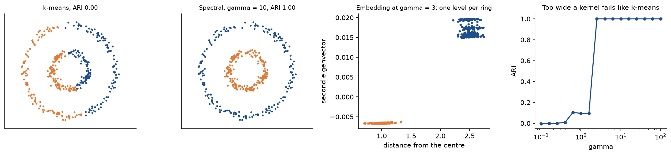
The third panel is the embedding k-means sees: each ring collapses to a narrow band at its own level, which any straight cut separates.

DBSCAN, mean shift and Gaussian mixtures

On two moons with 40 uniform noise points, the 4th-neighbour distance stays below 0.15 for 91 % of the points and shoots up for the last few dozen. ε = 0.2 with m = 5 finds the two moons exactly (ARI 1 on the moon points), with 413 core points, 9 border points and 18 noise points, all of them among the injected ones. The other 22 injected points fell close enough to a moon to be absorbed. Smaller ε fragments the moons (8 clusters at 0.1); larger merges them (1 cluster at 0.3).

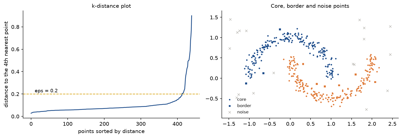
The knee of the curve is where ε should sit: below it the dense points, above it the points that are noise at any reasonable ε.

Mean shift on the four blobs finds 129 clusters at h = 0.3, 30 at 0.6, 9 at 0.8, 4 at 1.5 (ARI 0.9691), 3 from 2 to 3, 2 at 4 and 1 at 5.

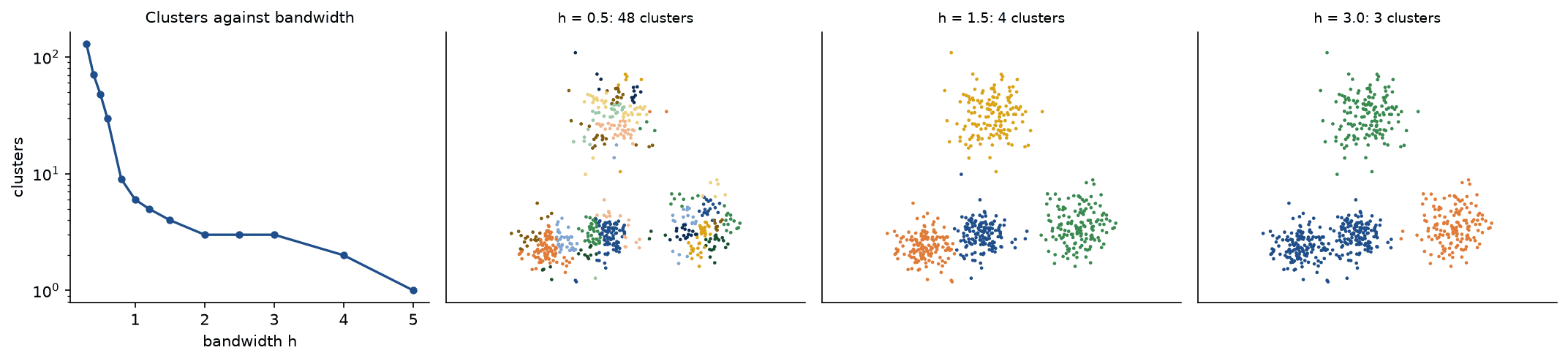
The plateau at three clusters is wider than the one at four, so a plateau rule would merge the close pair, the silhouette's answer.

A Gaussian mixture with full covariances recovers the stretched blobs exactly (ARI 1 against 0.5673 for k-means) in 21 EM iterations, with the log-likelihood per point rising from -1.6847 to -1.1361 and never falling. Only 0.2 % of the points have a largest responsibility below 0.9.

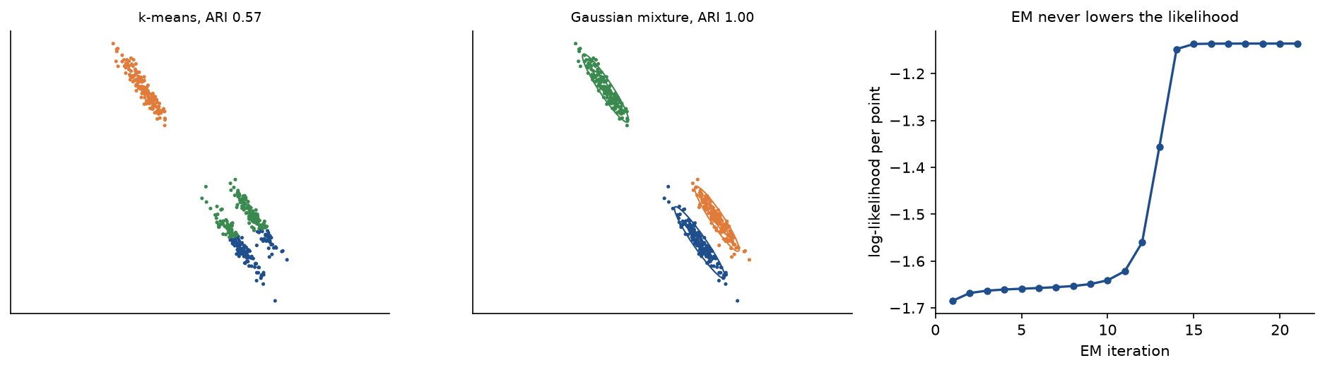
The likelihood creeps up for about ten iterations from the k-means start, which cuts across the stretched blobs, then rises sharply once the components align with them; it never steps down, as the Jensen argument requires.

k-means at scale

300,000 points from 20 overlapping blobs in 10 dimensions, k = 20, all runs from the same k-means++ seeds, on one thread:

• Our Lloyd: 90 iterations over all points, objective 3,006,856.7, in under ten seconds.
• Our mini-batch k-means with batches of 1,024 points: after 50 steps 3,152,101.8 (+4.83 %), after 200 steps 3,063,383.2 (+1.88 %) and after 800 steps 3,034,841.6 (+0.93 %), each in a fraction of a second. The adjusted Rand index of its partition with Lloyd's is 0.7755, 0.8239 and 0.8433.
• scikit-learn's KMeans from the same seeds stops at its default tolerance after 47 iterations with 3,006,867.0 (+0.00 %) in about a second, and MiniBatchKMeans stops after 535 steps, when its smoothed objective stalls, with 3,038,553.0 (+1.05 %).

Mini-batch k-means gets within 2 % of Lloyd's objective in a few per cent of the time; the partitions still differ noticeably, because with overlapping blobs many partitions have almost the same objective. The MapReduce formulation on 6,000 of these points in six splits reproduces Lloyd's centres in each of its 19 jobs to within 3 × 10⁻¹⁵, and the combiner reduces the records shuffled per job from 6,000 to 120, six splits times twenty clusters.

The same in scikit-learn and SciPy

Given the same inputs, every method agrees with its library counterpart:

• KMeans(init=centres, n_init=1, algorithm="lloyd", tol=0) gives identical labels and centres within 4 × 10⁻¹⁴ on the digits; on the nine points it also stops after 3 iterations at (3, 3), (5, 8) and (9, 3).
• kmeans_plusplus(n_local_trials=1) draws its second centre with our probabilities: over 4,000 seeds the frequencies match to within 0.02.
• scipy.cluster.hierarchy.linkage, leaves_list, cophenet and fcluster give the same linkage matrix to within 10⁻¹², the same leaf order, the same cophenetic distances and the same cuts for all four linkages on tie-free data, and AgglomerativeClustering the same partitions.
• DBSCAN gives identical labels and core points, and MeanShift the same centres to within 2 × 10⁻¹⁵ and identical labels.
• SpectralClustering with the Gaussian or the nearest-neighbour affinity gives the same partitions (ARI 1, also on the digits), and manifold.spectral_embedding the same embedding up to sign to within 10⁻⁶.
• GaussianMixture started from our initial parameters gives the same parameters to within 10⁻¹⁵ on the stretched blobs and the same number of iterations.
• adjusted_rand_score, rand_score, mutual_info_score, normalized_mutual_info_score with all four averages, silhouette_samples, davies_bouldin_score and calinski_harabasz_score agree to within 10⁻¹⁴.

Two disagreements are instructive, and both come from exact ties in integer pixel data. On the raw digits, single, average and Ward linkage agree with SciPy and scikit-learn, but complete linkage meets equal merge distances, breaks one tie differently, and from then on builds a different tree: our cut into ten clusters and scikit-learn's have an ARI of 0.8091, and SciPy's merge heights differ from ours by up to 1.5. With the ties broken by adding noise of size 10⁻⁶ to the pixels, all three implementations agree on every merge. Similarly, k-means on the digits from ten random data points meets a point exactly as far from two starting centres; scikit-learn computes distances by expanding the square, its rounding breaks the tie the other way, and although both runs end with identical labels, ours takes 15 iterations and scikit-learn's 16.

scikit-learn's KMeans reaches an objective of 1,165,188.9 on the digits with ten greedy starts in a few hundredths of a second, against our 1,165,146.6 with ten k-means++ starts in under a second; its default single greedy start gives 1,171,289.2.

When to use which:

• Use the from-scratch versions to learn the methods and to trace a result step by step, as format_lloyd_trace and format_linkage do.
• Use scikit-learn for real work. Its k-means is compiled and multithreaded and an order of magnitude faster than ours, its DBSCAN uses spatial trees, and HDBSCAN removes DBSCAN's single global ε. Use SciPy's linkage when you need the dendrogram.
• Use Spark MLlib's KMeans with k-means|| seeding when the data do not fit on one machine, and MiniBatchKMeans when they fit but are large.

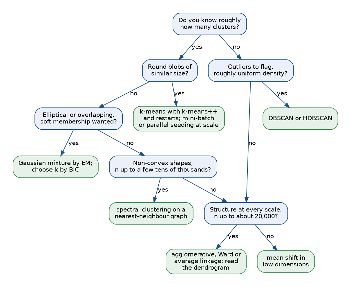
The tree is a starting point, not a rule: the method grid above shows how much the shape of the data decides, and it is usually worth running two methods that make different assumptions and comparing them.

Clustering is often a step inside a larger system rather than the end: colour quantization and superpixels in Segmentation, cluster-based features for Anomaly detection, and k-means on reduced features after Dimensionality reduction.

Pitfalls

• Unscaled features. Distance-based methods weigh each feature by its numeric range. Recording the second coordinate of the four blobs in units 100 times smaller drops k-means's ARI from 0.9691 to 0.3149; standardizing restores it. Standardizing is not automatically right either: if one feature's spread comes from the cluster separation itself, scaling it down hides the clusters. Decide the units deliberately (examples/common_mistakes.py).
• Choosing k by the smallest objective. J*(k) falls with every added centre and is zero at k = n. On 300 uniform points it falls smoothly from 48.21 to 5.97 over k = 1 to 8, and the mean silhouette is happy to report a best k = 4 (0.4042) on data with no clusters at all; the gap statistic answers k = 1. Every method returns clusters for noise.
• Trusting the silhouette on non-convex clusters. The silhouette rewards compact clusters. On the rings the true labels score 0.1598 and k-means's straight cut 0.3407; the Davies-Bouldin index, whose ring centres nearly coincide, prefers k-means even more strongly (1.1877 against 113.6621). Internal indices measure agreement with their own notion of a cluster.
• A silhouette that counts the point itself. a(i) averages over the other points of the cluster, dividing by the size minus one. Dividing by the size includes the zero distance from the point to itself and inflates every s(i): on the worked example the mean rises from 0.5470 to 0.6980. Averaging the per-cluster means instead of all points is a second slip: on the unequal-sizes data with the true labels the point average is 0.4989, but the average of the two cluster means (0.4663 and 0.8250) is 0.6457, because the 40-point cluster counts as much as the 400-point one.
• k-means++ with the wrong weights. The probabilities are proportional to D(x) squared, the squared distance to the nearest centre chosen so far, not to D(x) and not to the distance from the first centre only. With first centre A in the worked example, the D rule gives the second centre a probability of 0.0851 of landing in A's own group, more than three times the correct 0.0257. Distance lists computed by hand for this step are error-prone, and a slip in one entry changes every probability; recompute them in code, as tests/test_seeding.py does.
• One run of k-means. Lloyd's algorithm stops at the first fixed point it reaches. On the nine points 19 of 84 random starts end at a bad one, and on the 25-blob grid only one random run in 200 finds the best solution. Use k-means++, preferably greedy, and several restarts, and keep the lowest objective.
• Empty clusters. A centre that loses all its points has no mean; computing it anyway gives NaN centres that silently propagate. Our lloyd and scikit-learn move such a centre to a far point: started with one centre at (100, 100), far from all five blobs, lloyd still ends with three nonempty clusters and finite centres.
• Reading cluster numbers as class labels. Renaming the clusters of a perfect clustering drives "accuracy" to 0 while the ARI stays 1. The unadjusted Rand index has the opposite problem: random labels with ten clusters score 0.8195, against an ARI of -0.0015 and an NMI of 0.0158. Report the ARI or NMI, say which NMI average was used, and treat purity with suspicion, since singletons are perfectly pure.
• A kernel too wide for spectral clustering. Spectral clustering separates rings only when the similarity graph barely connects them. With γ up to 1.6 on our rings the result is the same kind of straight cut k-means gives, with an ARI of at most 0.11. A demonstration of spectral clustering that splits each ring into a left and a right half is showing this failure, not the method; check the eigenvalues, and if the first two are not well separated from the third, narrow the kernel or use a nearest-neighbour graph.
• DBSCAN's parameters and order. ε is in the units of the data, so it must be chosen after scaling, and one ε cannot fit clusters of different density. Border points within ε of two clusters go to whichever cluster the scan reaches first: for the nine points 0, 0.2, 0.4, 0.6, 1.5, 2.4, 2.6, 2.8 and 3.0 with ε = 0.95 and m = 4, the middle point joins the left group in the given order and the right group when the rows are reversed. Core points and noise never depend on the order.
• Mean shift's bandwidth. It decides everything: on the four blobs, 129 clusters at h = 0.3 and one at h = 5. The method is also quadratic in n and loses meaning in high dimension.
• Ward with arbitrary distances. Ward's merge cost, and the Lance-Williams update that computes it, assume Euclidean distances between points. Applied to a precomputed matrix of correlations or edit distances it still returns a tree, but not one that minimizes any sum of squares. Single linkage chains through noise bridges; centroid and median linkage can merge below an earlier merge.
• Ties in hierarchical clustering and k-means. Integer features create equal distances, and implementations break ties differently. On the digits, complete linkage gives a different tree from SciPy's and a ten-cluster cut with ARI 0.8091 against scikit-learn's. Report results that survive a tiny jitter, or at least report which library made them.
• A collapsing Gaussian component. EM maximizes a likelihood that is unbounded: with four copies of one point in the data and a component started on it, that component shrinks onto the copies, and the log-likelihood per point grows as the ridge shrinks: -4.3150 at reg_covar 10⁻³, -4.1790 at 10⁻⁶ and -3.9975 at 10⁻¹⁰, the last two higher than the -4.2784 of the sensible fit found with a ridge of 0.1. Without a ridge it would grow without limit. A higher likelihood is not a better clustering when a component has a weight of 4/203 and a variance equal to the ridge. Keep reg_covar positive and restart from several initializations.

Further reading

• S. P. Lloyd, "Least squares quantization in PCM", IEEE Transactions on Information Theory 28(2), 129-137, 1982. The algorithm, written in 1957.
• J. MacQueen, "Some methods for classification and analysis of multivariate observations", Proceedings of the Fifth Berkeley Symposium on Mathematical Statistics and Probability, 281-297, 1967. The name k-means.
• D. Arthur and S. Vassilvitskii, "k-means++: the advantages of careful seeding", Proceedings of the ACM-SIAM Symposium on Discrete Algorithms, 1027-1035, 2007.
• B. Bahmani, B. Moseley, A. Vattani, R. Kumar and S. Vassilvitskii, "Scalable k-means++", Proceedings of the VLDB Endowment 5(7), 622-633, 2012. k-means||.
• D. Sculley, "Web-scale k-means clustering", Proceedings of the International World Wide Web Conference, 1177-1178, 2010. Mini-batch k-means.
• D. Aloise, A. Deshpande, P. Hansen and P. Popat, "NP-hardness of Euclidean sum-of-squares clustering", Machine Learning 75(2), 245-248, 2009.
• A. Vattani, "k-means requires exponentially many iterations even in the plane", Discrete and Computational Geometry 45(4), 596-616, 2011.
• P. J. Rousseeuw, "Silhouettes: a graphical aid to the interpretation and validation of cluster analysis", Journal of Computational and Applied Mathematics 20, 53-65, 1987.
• R. Tibshirani, G. Walther and T. Hastie, "Estimating the number of clusters in a data set via the gap statistic", Journal of the Royal Statistical Society B 63(2), 411-423, 2001.
• J. H. Ward, "Hierarchical grouping to optimize an objective function", Journal of the American Statistical Association 58(301), 236-244, 1963.
• G. N. Lance and W. T. Williams, "A general theory of classificatory sorting strategies: 1. Hierarchical systems", The Computer Journal 9(4), 373-380, 1967.
• D. Müllner, "Modern hierarchical, agglomerative clustering algorithms", arXiv:1109.2378, 2011. The algorithms behind SciPy's linkage.
• M. Ester, H.-P. Kriegel, J. Sander and X. Xu, "A density-based algorithm for discovering clusters in large spatial databases with noise", Proceedings of the International Conference on Knowledge Discovery and Data Mining, 226-231, 1996.
• E. Schubert, J. Sander, M. Ester, H.-P. Kriegel and X. Xu, "DBSCAN revisited, revisited: why and how you should (still) use DBSCAN", ACM Transactions on Database Systems 42(3), 19, 2017.
• R. J. G. B. Campello, D. Moulavi and J. Sander, "Density-based clustering based on hierarchical density estimates", Pacific-Asia Conference on Knowledge Discovery and Data Mining, 160-172, 2013. HDBSCAN.
• K. Fukunaga and L. Hostetler, "The estimation of the gradient of a density function, with applications in pattern recognition", IEEE Transactions on Information Theory 21(1), 32-40, 1975.
• D. Comaniciu and P. Meer, "Mean shift: a robust approach toward feature space analysis", IEEE Transactions on Pattern Analysis and Machine Intelligence 24(5), 603-619, 2002.
• J. Shi and J. Malik, "Normalized cuts and image segmentation", IEEE Transactions on Pattern Analysis and Machine Intelligence 22(8), 888-905, 2000.
• A. Y. Ng, M. I. Jordan and Y. Weiss, "On spectral clustering: analysis and an algorithm", Advances in Neural Information Processing Systems 14, 2001.
• U. von Luxburg, "A tutorial on spectral clustering", Statistics and Computing 17(4), 395-416, 2007. The RatioCut and Ncut relaxations in full.
• A. P. Dempster, N. M. Laird and D. B. Rubin, "Maximum likelihood from incomplete data via the EM algorithm", Journal of the Royal Statistical Society B 39(1), 1-38, 1977.
• L. Hubert and P. Arabie, "Comparing partitions", Journal of Classification 2, 193-218, 1985. The adjusted Rand index.
• N. X. Vinh, J. Epps and J. Bailey, "Information theoretic measures for clusterings comparison", Journal of Machine Learning Research 11, 2837-2854, 2010.
• J. Kleinberg, "An impossibility theorem for clustering", Advances in Neural Information Processing Systems 15, 2002.
• C. M. Bishop, Pattern Recognition and Machine Learning, chapter 9, Springer, 2006. k-means, mixtures and EM.
• T. Hastie, R. Tibshirani and J. Friedman, The Elements of Statistical Learning, second edition, section 14.3, Springer, 2009.