Information theory

Machine learning measures uncertainty all the time, often without saying so. A decision tree picks the split that removes the most uncertainty about the label, a classifier is trained by minimizing the average surprise of the true labels under its predictions, a language model is compared with another by its perplexity, and a compressor is judged by how close it gets to a limit nobody can beat. All of these are the same few quantities: self-information, entropy, mutual information, cross-entropy and the Kullback-Leibler divergence. This page derives each of them, shows how they fit together, and works them through by hand on a sixteen-day riding log, a weather forecast, a classifier, a sentence and a five-letter code. It implements everything in NumPy, checks it against SciPy and scikit-learn, measures how biased entropy estimates from samples are, codes a source whose entropy rate is known exactly, and finally selects the pixels that identify a handwritten digit. Afterwards you will be able to compute every one of these quantities on paper, explain why minimizing cross-entropy is maximum likelihood and why the two directions of the KL divergence fit differently, choose and trust a mutual-information score, and say how many bits a code can possibly save. It builds on Probability and statistics.

To run the code in this topic, install the base group, and the ml group for the comparisons with SciPy and scikit-learn and for the sample project.

Intuition

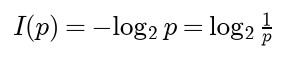
An outcome that was certain tells you nothing when it happens. An outcome you thought unlikely tells you a lot. Information theory turns this into a number, the self-information of an outcome: minus the logarithm of its probability. In base 2 the unit is the bit. A fair coin flip is worth one bit, a fair die roll log2 6 = 2.5850 bits, and a one-in-a-hundred event 6.6439 bits. One bit is the information in the answer to a yes or no question whose two answers were equally likely, so an outcome of probability one half to the power k settles exactly k such questions.

The entropy of a random variable is its average self-information, how surprised you expect to be. It is zero when one outcome is certain and largest when all outcomes are equally likely. It also answers a practical question: how many bits per symbol does the best possible code need? No code can beat the entropy on average, and good codes come arbitrarily close.

Everything else follows from comparing averages:

• Knowing one variable can make another less uncertain. The drop in entropy is the mutual information, the number of bits one variable tells you about the other. A decision tree computes it for every candidate split and calls it information gain.
• If you believe the probabilities are q while they are really p, your average surprise is the cross-entropy H(p, q), never less than the entropy H(p). The difference is the KL divergence, the price of the wrong model in bits per observation. Training a classifier by minimizing cross-entropy drives this price down, and that is exactly maximum likelihood.
• A code designed for q and used on data from p costs about H(p, q) bits per symbol, so the KL divergence is literally the number of bits wasted per symbol.

The map shows how the quantities are built from one another, in blue, and where each is used, in green. The dashed arrow is the identity that ties the two branches together: mutual information is itself a KL divergence, of the joint distribution from the product of its marginals.

How it works

Notation

X and Y are discrete random variables with values x and y. The quantities on this page are:

• p(x), p(x, y) and p(y | x): the probability, the joint probability and the conditional probability.
• p and q: two distributions over the same K outcomes. p is the truth or the data, q a model.
• log: the logarithm in some base. log2 measures in bits and the natural logarithm ln in nats, and one nat is 1 / ln 2 = 1.4427 bits.
• H(X) or H(p): the entropy of a variable or of a distribution. H(X, Y) is the joint entropy and H(Y | X) the conditional entropy.
• I(X; Y): the mutual information. H(p, q): the cross-entropy.
• KL(p ‖ q): the Kullback-Leibler divergence of q from p. The formula images write it as D with the subscript KL.
• ℓi and L: the length in bits of the codeword for outcome i, and the average length L, the sum of pi ℓi.
• n and p̂: the sample size and the empirical distribution of a sample, the fraction of the sample equal to each value.

The formula images write indices as subscripts; the text writes them plainly, as p1, ℓ2 or X1, ..., Xk. Sums run over outcomes with positive probability, which is the same as the convention that 0 log 0 = 0, the limit of t log t as t goes to zero.

Self-information and its axioms

Which function I(p) should measure the information in an outcome of probability p in (0, 1]? Four requirements pin it down:

1. A certain outcome carries no information: I(1) = 0.
2. Rarer outcomes carry more: I is decreasing.
3. Information from independent outcomes adds. Two independent events of probabilities p and q occur together with probability pq, so I(pq) = I(p) + I(q).
4. Small changes in probability make small changes in information: I is continuous.

Substituting p = 2 to the power -t turns requirement 3 into Cauchy's functional equation for a function f of t ≥ 0, and the rest is algebra:

Induction gives the rule for whole multiples, dividing gives it for rational numbers, and continuity extends it to every t. Requirement 2 forces c > 0, and requirement 1 holds automatically. The constant only chooses the unit, and c = 1 gives bits:

With the natural logarithm the same formula measures in nats, and base 10 gives hartleys, which are rarely used.

Entropy

The entropy of X is the expected self-information of its outcome:

It depends only on the probabilities, not on the values of X, which is why it is also written H(p). Each term -p log p is non-negative for p between 0 and 1, so H(X) ≥ 0, with equality exactly when one outcome has probability one. Changing the base of the logarithm multiplies the entropy by a constant: the entropy in bits is the entropy in nats divided by ln 2.

Entropy is largest for the uniform distribution. Jensen's inequality for the concave logarithm says that the average of log Z is at most the logarithm of the average of Z. Applied to Z = 1 / p(X) it gives

Equality in Jensen's inequality needs 1 / p(x) to be the same for every outcome with positive probability, and equality in the last step needs all K outcomes to have positive probability, so H(X) = log K exactly when p is uniform. Four equally likely outcomes have 2 bits of entropy; any other distribution on four outcomes has less.

For two outcomes with probabilities p and 1 - p the entropy is the binary entropy:

It is zero at p = 0 and p = 1, one bit at p = 1/2, and symmetric about 1/2. Its slope is minus the log-odds, infinite at both ends.

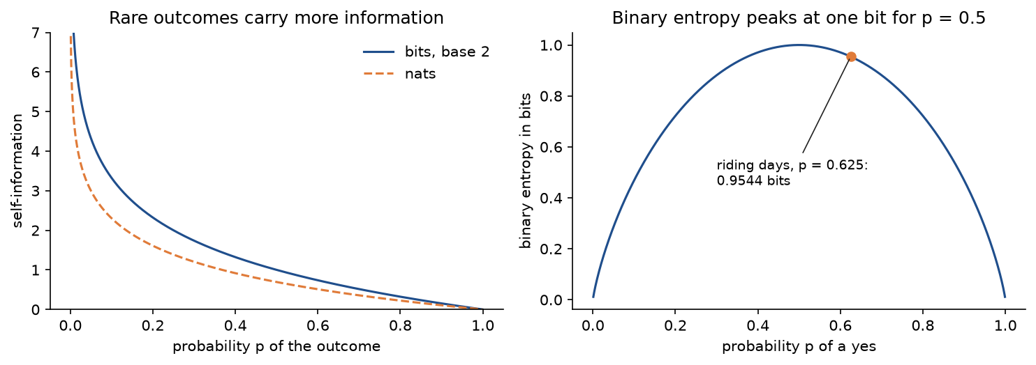
The left panel shows that bits and nats differ by the constant factor ln 2 = 0.6931 and nothing else. The right panel shows how flat the binary entropy is near its peak: the cyclist of the worked example rides on 62.5 % of days and her riding decision still has 0.9544 bits of entropy, almost as much as a fair coin.

Joint entropy, conditional entropy and the chain rule

The joint entropy H(X, Y) is the entropy of the pair, minus the sum of p(x, y) log p(x, y). The conditional entropy of Y given X is the entropy of Y that remains once X is known, averaged over the values of X:

Taking the logarithm of the product rule p(x, y) = p(x) p(y | x) and averaging minus both sides over p(x, y) gives the chain rule:

The uncertainty about the pair is the uncertainty about the first variable plus what remains about the second once the first is known. Applied repeatedly, the entropy of X1, ..., Xk is the sum over i of the entropy of Xi given all the variables before it.

Mutual information

The mutual information between X and Y is the reduction in the uncertainty about Y from learning X. The chain rule rewrites it in the other forms, and writing the entropies as averages over p(x, y) and collecting the logarithms gives the last one:

The symmetric forms say that X tells you as much about Y as Y tells you about X. The last form is the divergence of the joint distribution from the product of its marginals. The next section shows that a KL divergence is never negative and is zero only for identical distributions, so I(X; Y) ≥ 0, with equality exactly when X and Y are independent. Two consequences follow: conditioning never increases entropy on average, H(Y | X) ≤ H(Y), and I(X; X) = H(X), since a variable tells you everything about itself. The information diagram in the worked example shows the five quantities as overlapping bars.

Information gain is this quantity estimated from data. A data set D with class labels is split by an attribute A into subsets Dv, one per value v of the attribute:

Here H(D) is the entropy of the class frequencies in D. The first term is H(Y) and the sum is H(Y | A), both computed from the empirical distribution, so the gain is the plug-in estimate of I(A; Y). ID3 and C4.5 split each node on the attribute with the largest gain; Decision trees builds them. The gain ratio of the second line divides by the entropy of the subset sizes to penalize attributes with many values.

As a measure of feature relevance, I(Xj; Y) has two virtues over correlation: it detects any kind of dependence, not only a linear one, and it does not care how the values of Xj are labelled. With X uniform on -2, -1, 0, 1 and 2 and Y = X squared, the correlation is exactly zero, because the averages of X and of X cubed are both zero, while X determines Y and I(X; Y) = H(Y) = H(0.2, 0.4, 0.4) = 1.5219 bits. Its limits appear under Pitfalls: it scores one feature at a time, and estimated from few samples it is biased upwards, more so for features with many values.

Cross-entropy and KL divergence

Suppose outcomes are drawn from p but you assign them the probabilities q. Your average surprise is the cross-entropy, and the excess over the unavoidable surprise H(p) is the Kullback-Leibler divergence:

Gibbs' inequality says that KL(p ‖ q) ≥ 0, with equality only when q = p. The proof needs one fact: ln t ≤ t - 1 for every t > 0, with equality only at t = 1, because the line t - 1 is tangent to the concave curve ln t at t = 1. Summing over the outcomes with p(x) > 0,

Equality needs q(x) = p(x) wherever p(x) > 0, and then q has no mass left for anything else. In another base the divergence is multiplied by a positive constant, which changes nothing. Three facts follow at once: the cross-entropy is never below the entropy, mutual information is never negative, and the divergence of p from the uniform distribution is log K - H(p), a second proof that the uniform distribution has the largest entropy.

The KL divergence is not a distance. It is not symmetric, it violates the triangle inequality, and it is infinite as soon as q(x) = 0 for an outcome with p(x) > 0: a model that rules out something that happens is infinitely wrong. A symmetric and bounded alternative is the Jensen-Shannon divergence, which compares both distributions with their average:

It lies between 0 and 1 bit, it is finite because m has mass wherever p or q has, and its square root is a metric.

Forward and reverse KL

When q comes from a restricted family, such as single Gaussians, and p does not, the two directions of the divergence pick different best fits:

• The forward divergence averages over p. Wherever p has mass and q has almost none, -log q(x) is huge, so the best q spreads out to cover all of p: it is mass-covering, or mean-seeking.
• The reverse divergence averages over q. Wherever q puts mass and p has almost none, -log p(x) is huge, so the best q stays inside a region where p is large and ignores the rest: it is mode-seeking, or zero-forcing, and it can have one local minimum per mode.

For a Gaussian q with mean μ and variance σ² the forward fit has a closed form. Substituting the log density of the Gaussian into the forward divergence gives the first line below:

Setting the derivative with respect to μ to zero gives the mean of p, and then the derivative with respect to σ gives the variance of p. The forward fit matches the mean and the variance of p, however many modes p has. Between two Gaussians the divergence in nats is

and the tests use it to check the grid on which the fits of the worked example are computed. Forward KL is what maximum likelihood minimizes, as the next section shows. Reverse KL appears where q must be sampled from or integrated against while p can only be evaluated up to a constant, as in variational inference, and in the penalty that keeps a fine-tuned language model close to its reference model in Preference tuning.

Minimizing cross-entropy is maximum likelihood

Let x1, ..., xn be data and qθ a model with parameters θ. The average negative log-likelihood groups equal data points, and each distinct value x appears a fraction p̂(x) of the time:

The entropy of p̂ does not depend on θ, so maximizing the likelihood, minimizing the cross-entropy between data and model and minimizing the forward KL divergence from the data to the model are the same optimization. If the model can represent any distribution on the outcomes, Gibbs' inequality puts the minimum at qθ = p̂: the maximum-likelihood estimate of a categorical distribution is the table of observed frequencies, and the minimum value is the entropy of the data. As n grows, p̂ approaches the true p and the procedure minimizes the forward divergence from p over the model family.

A classifier models a conditional distribution qθ(y | x). The same argument applied to each example, with the observed label as a distribution that puts all its mass on yi, gives the training loss of logistic regression and of every softmax network:

Logistic regression derives its gradient and Loss functions compares it with the squared error.

Log loss and perplexity

The log loss of a classifier is that average, in nats by convention, with ŷi the predicted probability of class 1 in the binary case:

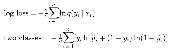
It is a strictly proper scoring rule: if the labels really follow p(y | x), the expected log loss of a prediction q is H(p, q), smallest only at q = p, so it rewards honest, calibrated probabilities rather than confident ones.

Perplexity turns an average log loss back into a number of choices:

It is the inverse of the geometric mean of the probabilities given to what actually happened. A model that spreads its probability evenly over k options at every step has perplexity exactly k, so a perplexity of 20 means the model is, on average, as uncertain as a uniform choice among 20 tokens. For a language model the wi are the tokens of held-out text, usually including an end-of-sentence marker; N-gram language models and A tiny GPT use it to compare models. Because the expected cross-entropy is never below the entropy, no model of a source can have a long-run perplexity below 2 to the power H, where for text H is the entropy rate defined below.

Codes and the Kraft inequality

A binary code gives every outcome i a codeword, a string of ℓi bits, and encodes a message by concatenating codewords. The code is prefix-free if no codeword is the beginning of another; then a decoder can read bits until they form a codeword, emit the symbol and start again, with no separators. Prefix-free codes are exactly the codes whose codewords are the leaves of a binary tree, reading 0 for one branch and 1 for the other. The Kraft inequality says that a prefix-free binary code with lengths ℓ1, ..., ℓK exists if and only if

Necessity: let ℓmax be the longest length. A codeword of length ℓi is the beginning of 2 to the power ℓmax - ℓi of the strings of length ℓmax, and because no codeword begins another these sets of strings are disjoint, so

and dividing by 2 to the power ℓmax gives the inequality. Sufficiency: sort the lengths in increasing order and give each outcome the first string of its length that does not start with an earlier codeword. Equivalently, start with the code 0, add one after each codeword, and append zeros whenever the length grows; the inequality guarantees that this canonical construction never runs out of strings, and it is how canonical_code assigns codewords. McMillan's theorem extends the inequality to every uniquely decodable code, so restricting attention to prefix-free codes loses nothing.

Entropy bounds the average code length

For any lengths that satisfy the Kraft inequality, let c be their Kraft sum and define the distribution r implied by the code. Then the excess of the average length over the entropy is a divergence minus the logarithm of c:

Both terms are non-negative, so L ≥ H(p): no prefix-free code, and by McMillan no uniquely decodable code, beats the entropy on average. Equality needs c = 1 and pi = 2 to the power -ℓi, which is possible only when every probability is a power of one half. For a complete code, with Kraft sum one, the excess is exactly the divergence of the implied distribution from p.

The bound is nearly achievable. The Shannon code rounds every self-information up to a whole number of bits:

Each length is less than -log2 pi + 1, which gives the upper bound, and the optimal code is at least as good. The extra bit is a rounding loss per codeword, and it can be spread over many symbols. Coding blocks of k independent symbols as single outcomes, the block has entropy kH, so

This is the source coding theorem: for a memoryless source the entropy is the smallest achievable average number of bits per symbol, and it can be approached as closely as desired. For a source with memory the limit is the entropy rate. For a stationary first-order Markov chain with transition matrix P and stationary distribution π it has a closed form, and the entropy of a block grows by exactly the rate for every letter after the first:

The rate is smaller than the entropy H(π) of a single letter whenever successive letters depend on each other. Coding with the wrong model costs the cross-entropy:

The KL divergence is the number of extra bits per symbol paid for believing q. A compressor is a probability model in disguise, and the cross-entropy of a model on data is the length an ideal coder, such as an arithmetic coder, would reach with it.

Huffman's algorithm

Huffman's algorithm builds an optimal prefix-free code. Start with one node per outcome, weighted by its probability. Repeatedly remove the two nodes of smallest weight and replace them by a parent whose weight is their sum, until one node is left. Each merge adds one bit to the codeword of every outcome below the merged nodes, so the code lengths are the depths of the leaves.

Why it is optimal, in outline. In some optimal code the two least probable outcomes have the longest codewords and differ only in the last bit: if a more probable outcome had a longer codeword, swapping the two would shorten the average, and a longest codeword without a sibling could lose its last bit. Merging those two outcomes into one of probability pa + pb gives a problem with one outcome fewer, whose optimal average length is exactly L - (pa + pb). By induction Huffman's construction solves the smaller problem optimally, and splitting the merged node back adds the same pa + pb. Huffman codes therefore satisfy H ≤ L < H + 1, never lose to the Shannon code, and have Kraft sum exactly one. Entropy coding covers Huffman, arithmetic and dictionary coding in depth, and JPEG from scratch uses Huffman tables in a real format.

Estimating entropy from samples

In practice the probabilities are unknown and estimated from n samples. The plug-in estimate replaces p by the observed frequencies p̂ and computes H(p̂). It is biased low. Entropy is a concave function of the distribution and p̂ is an unbiased estimate of p, so Jensen's inequality gives the first line below for every sample size. A second-order Taylor expansion of H(p̂) around p gives the size of the bias:

The first-order term has expectation zero because p̂ is unbiased. The matrix of second derivatives is diagonal, with entries -1 / pk, so only the variances of the frequencies enter, and K is the number of outcomes of positive probability. The Miller-Madow estimate adds this back, using the number K̂ of outcomes actually observed:

The expansion assumes many samples per outcome. When n is comparable to K the formula is no longer accurate, Miller-Madow leaves much of the bias in place, and estimators designed for that regime, such as those of Chao and Shen or of Nemenman, Shafee and Bialek, are needed.

The plug-in mutual information is biased the other way. Writing it as the sum of the two marginal plug-in entropies minus the joint one and applying the bias formula to each term, for independent variables with a and b equally possible values,

This is no coincidence: 2n times the plug-in mutual information in nats is the G-statistic of the likelihood-ratio test of independence, which has approximately a chi-square distribution with (a - 1)(b - 1) degrees of freedom when the variables are independent (Probability and statistics). The mean of that distribution, divided by 2n, is the formula above. An estimated mutual information therefore means little until it is compared with that baseline or with the scores obtained after shuffling one variable.

examples/estimation_bias.py measures both biases. A variable with sixteen values and probabilities proportional to 1 / k, entropy 3.4032 bits, is sampled n times, 4000 times for each n. The mean bias of the estimates in bits, against the first-order prediction, is:

• n = 8: plug-in -1.1624, Miller-Madow -0.7665, predicted -1.3525.
• n = 32: plug-in -0.3776, Miller-Madow -0.1449, predicted -0.3381.
• n = 128: plug-in -0.0867, Miller-Madow -0.0045, predicted -0.0845.
• n = 1024: plug-in -0.0098, Miller-Madow 0.0007, predicted -0.0106.

Once there are several samples per value the formula is accurate and Miller-Madow removes nearly all the bias; with fewer samples than values both fall short. Two independent variables with 8 and 4 equally likely values have zero mutual information, yet the plug-in estimate averages 0.9190 bits from 16 samples, 0.0612 from 256 and 0.0037 from 4096, against 0.9468, 0.0592 and 0.0037 from the formula converted to bits.

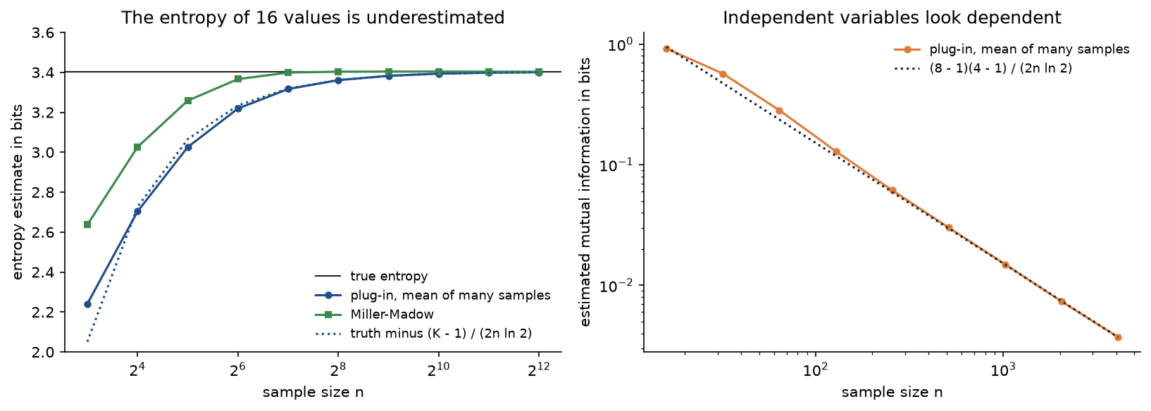
The left panel shows the plug-in entropy approaching the truth from below like 1 / n, and the right panel shows that the mutual information of independent variables is never estimated as zero: on logarithmic axes it falls along a straight line exactly where the formula says.

Worked example

Every value below is computed in double precision and rounded to four decimals for display. Sums written out from rounded terms agree with the full-precision values unless the text says otherwise. Logarithms are base 2 unless stated.

Entropies of a riding log

A cyclist logs sixteen days: the sky in the morning, the wind, and whether she rode to work.

• Clear sky on 6 days: she rode on 5 and stayed home on 1.
• Cloudy sky on 5 days: rode on 4, stayed on 1.
• Rain on 5 days: rode on 1, stayed on 4.
• Calm wind on 9 days: rode on 7, stayed on 2.
• Windy on 7 days: rode on 3, stayed on 4.

She rode on 10 of the 16 days, so the entropy of the riding decision is (10/16) log2(16/10) + (6/16) log2(16/6) = 0.625 × 0.6781 + 0.375 × 1.4150 = 0.4238 + 0.5306 = 0.9544 bits, a little under the one bit of a fair coin. The sky has three values with probabilities 6/16, 5/16 and 5/16, close to uniform: each 5-day value contributes (5/16) log2(16/5) = 0.5244, so H(sky) = 0.5306 + 2 × 0.5244 = 1.5794 bits, just below log2 3 = 1.5850. The wind has H(wind) = 0.9887 bits.

Information gain of two candidate splits

Splitting the days by the sky gives three groups:

• Clear, 5 rides in 6 days: H = (5/6) log2(6/5) + (1/6) log2 6 = 0.2192 + 0.4308 = 0.6500.
• Cloudy, 4 in 5, and rain, 1 in 5, have the same entropy: 0.8 log2 1.25 + 0.2 log2 5 = 0.2575 + 0.4644 = 0.7219.

Weighting each by its share of the days, H(ride | sky) = (6/16) × 0.6500 + (5/16) × 0.7219 + (5/16) × 0.7219 = 0.2438 + 0.2256 + 0.2256 = 0.6950, and the gain is 0.9544 - 0.6950 = 0.2595 bits. The difference of the rounded values is 0.2594; the full-precision gain is 0.2595.

Splitting by the wind instead, calm days have H = (7/9) log2(9/7) + (2/9) log2(9/2) = 0.2820 + 0.4822 = 0.7642 and windy days H = (3/7) log2(7/3) + (4/7) log2(7/4) = 0.5239 + 0.4613 = 0.9852. Weighted, H(ride | wind) = (9/16) × 0.7642 + (7/16) × 0.9852 = 0.4299 + 0.4310 = 0.8609, and the gain is 0.0935 bits.

A tree would split on the sky first. Two remarks. Windy days alone are more uncertain than the log as a whole, 0.9852 against 0.9544: conditioning lowers entropy on average, not for every value. And the day number, used as an attribute, puts each day in its own pure group, so its gain is the whole 0.9544 bits, the largest possible, although it predicts nothing about a new day.

Mutual information and the chain rule

The joint counts of sky and riding are 1 and 5 on clear days, 1 and 4 on cloudy days and 4 and 1 on rainy days, for stayed and rode. A count c out of 16 contributes (c/16) log2(16/c) to the joint entropy: 0.25 for c = 1, 0.5 for c = 4 and 0.5244 for c = 5, so H(sky, ride) = 0.5244 + 3 × 0.25 + 2 × 0.5 = 2.2744 bits.

The chain rule holds in both orders: H(sky) + H(ride | sky) = 1.5794 + 0.6950 = 2.2744, and H(ride) + H(sky | ride) = 0.9544 + 1.3200 = 2.2744. The mutual information is H(ride) - H(ride | sky) = H(sky) - H(sky | ride) = 0.2595 bits = 0.1799 nats, the information gain of the sky split, as it must be. Either difference of rounded values gives 0.2594; the full-precision value is 0.2595.

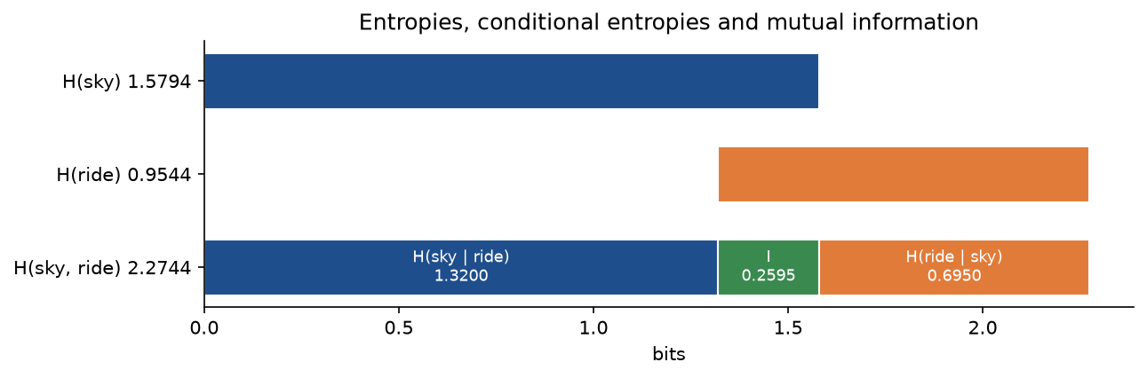
The two upper bars overlap exactly over the green segment, the mutual information, and the parts outside the overlap are the two conditional entropies. Their total along the bottom bar is the joint entropy, which is the chain rule drawn as lengths.

Cross-entropy and KL divergence of a forecast

In a town the sky is clear, cloudy or rainy with probabilities p = (0.5, 0.25, 0.25), and a forecaster's model says q = (0.7, 0.2, 0.1). The entropy is H(p) = 0.5 × 1 + 0.25 × 2 + 0.25 × 2 = 1.5 bits. The model's surprises, -log2 q, are 0.5146, 2.3219 and 3.3219 bits, so

• H(p, q) = 0.5 × 0.5146 + 0.25 × 2.3219 + 0.25 × 3.3219 = 0.2573 + 0.5805 + 0.8305 = 1.6683 bits.
• KL(p ‖ q), the sum of p log2(p / q), is -0.2427 + 0.0805 + 0.3305 = 0.1683 bits, which is 1.6683 - 1.5.

The first term of the divergence is negative: the model gives clear skies more probability than they deserve, which on clear days makes it less surprised than the truth would be. The divergence as a whole is still positive. In the other direction, H(q) = 1.1568, H(q, p) = 0.7 × 1 + 0.2 × 2 + 0.1 × 2 = 1.3, and KL(q ‖ p) = 0.3398 - 0.0644 - 0.1322 = 0.1432 bits, not 0.1683. In nats, KL(p ‖ q) = 0.1683 × ln 2 = 0.1166.

Cross-entropy as maximum likelihood, on the riding log: a model that rides with probability θ has average negative log-likelihood -((10/16) log2 θ + (6/16) log2(1 - θ)), the cross-entropy between the observed frequencies and the model. On a grid of θ values from 0.01 to 0.99 its minimum is at θ = 0.6250 = 10/16, the observed frequency, and the minimum value is 0.9544 bits, the entropy of the data.

Forward and reverse KL fits

The target is a mixture of two Gaussians, with weight 0.6 on mean -1.5 and standard deviation 0.5 and weight 0.4 on mean 2 and standard deviation 0.7. The model is a single Gaussian. Moment matching gives the forward fit by hand: the mean is 0.6 × (-1.5) + 0.4 × 2 = -0.1, and the variance is the mixture's second moment minus the squared mean, 0.6 × (0.25 + 2.25) + 0.4 × (0.49 + 4) - 0.01 = 3.286, so the standard deviation is 1.8127. The reverse fits come from numerical minimization on a grid (see The code). Each fit below gives its mean and standard deviation, then the forward and the reverse divergence in nats:

• Forward, the global minimum: mean -0.1000, standard deviation 1.8127, forward 0.4852, reverse 1.0624.
• Reverse on the left mode, the global minimum: -1.4937, 0.5092, forward 8.7975, reverse 0.5071.
• Reverse between the modes, a local minimum: 0.4857, 1.6024, forward 0.5685, reverse 0.8503.
• Reverse on the right mode, a local minimum: 1.9756, 0.7348, forward 6.1151, reverse 0.9073.

The forward fit straddles both modes and puts its peak where p has almost no mass. The best reverse fit sits on the heavier mode and ignores the other one, which costs it 8.7975 nats in the forward direction. Its reverse divergence, 0.5071, is close to -ln 0.6 = 0.5108, the value it would have if q were exactly the left component, because p is about 0.6 q wherever q has mass. A gradient method minimizing the reverse divergence would stop in whichever of its three basins it started in.

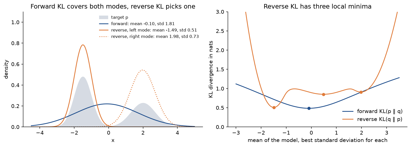
The left panel shows what each direction rewards, and the right panel why the reverse fit depends on its starting point: its profile has three valleys, the forward one only one.

Log loss and perplexity

A binary classifier predicts the probabilities 0.9, 0.7, 0.2 and 0.6 of class 1 for four examples whose labels are 1, 1, 0 and 0. The probabilities it gave the true labels are 0.9, 0.7, 0.8 and 0.4, the last example being a mistake. The losses are -ln 0.9 = 0.1054, -ln 0.7 = 0.3567, -ln 0.8 = 0.2231 and -ln 0.4 = 0.9163 nats, so the log loss is their mean, 0.4004 nats or 0.5776 bits. The product of the four probabilities is 0.2016, and the perplexity is e to the power 0.4004, equally 0.2016 to the power -1/4, which is 1.4924. One wrong example contributes more than half of the loss. Always predicting 0.5 would score ln 2 = 0.6931 nats and perplexity 2.

A bigram language model scores the held-out sentence "rain stops the race" followed by an end marker with five predictions: rain after the start of a sentence with probability 0.25, stops after rain 0.5, the after stops 0.125, race after the 0.4, and the end marker after race 0.2. In bits these cost 2, 1, 3, 1.3219 and 2.3219, together log2 800 = 9.6439 bits because the product of the five probabilities is 1/800 (the rounded terms sum to 9.6438). That is 1.9288 bits per token, and the perplexity is 2 to the power 1.9288, equally 0.00125 to the power -1/5, which is 3.8073. The model is as uncertain as a uniform choice among 3.8 words at each step; a model that spreads its probability over a twelve-word vocabulary has perplexity 12.

A Huffman code

Five letters occur with probabilities A 0.45, B 0.25, C 0.14, D 0.09 and E 0.07. Huffman's algorithm merges

1. E (0.07) and D (0.09) into DE (0.16),
2. C (0.14) and DE (0.16) into CDE (0.30),
3. B (0.25) and CDE (0.30) into BCDE (0.55),
4. A (0.45) and BCDE (0.55) into the root (1.00).

Reading the branch labels from the root to a leaf spells its codeword, and each internal node is labelled with the merge that created it. For each letter, the self-information -log2 p, the Huffman codeword and the Shannon code length are:

• A: 1.1520 bits, codeword 0, Shannon length 2.
• B: 2.0000 bits, codeword 10, Shannon length 2.
• C: 2.8365 bits, codeword 110, Shannon length 3.
• D: 3.4739 bits, codeword 1110, Shannon length 4.
• E: 3.8365 bits, codeword 1111, Shannon length 4.

The Kraft sum of the Huffman lengths is 1/2 + 1/4 + 1/8 + 1/16 + 1/16 = 1, a complete code. The average length is L = 0.45 × 1 + 0.25 × 2 + 0.14 × 3 + 0.09 × 4 + 0.07 × 4 = 0.45 + 0.5 + 0.42 + 0.36 + 0.28 = 2.01 bits, and the entropy is H = 0.45 × 1.1520 + 0.25 × 2 + 0.14 × 2.8365 + 0.09 × 3.4739 + 0.07 × 3.8365 = 1.9967 bits. The code wastes L - H = 0.0133 bits per letter, an efficiency H / L of 0.9934, where a fixed-length code would need 3 bits. Because the code is complete, the waste is exactly the KL divergence of r = (1/2, 1/4, 1/8, 1/16, 1/16), the distribution the lengths imply, from p. The Shannon code gives A two bits instead of one, has Kraft sum 0.75 and averages 2.46 bits, between H and H + 1 but worse than Huffman.

The message BADCAE encodes as 10, 0, 1110, 110, 0 and 1111, which concatenate to 100111011001111: 15 bits instead of 18, decoded unambiguously from left to right because no codeword begins another.

A code is only as good as its model. Used on a source in which all five letters are equally likely, with entropy log2 5 = 2.3219 bits, the same code averages 0.2 × (1 + 2 + 3 + 4 + 4) = 2.8 bits per letter, and the excess is the divergence of r from the uniform distribution, 0.4781 bits.

Estimating entropy from ten draws

Ten draws from a variable with four equally likely values, true entropy 2 bits, produce the counts 5, 3, 2 and 0. The plug-in estimate is H(0.5, 0.3, 0.2) = 0.5 × 1 + 0.3 × 1.7370 + 0.2 × 2.3219 = 1.4855 bits, half a bit short. Three values were seen, so Miller-Madow adds (3 - 1) / (2 × 10) = 0.1 nats, which is 0.1443 bits, giving 1.6297 bits: better, still short, because ten draws are far too few for a correction derived for large samples.

Every number in this section is asserted by tests/test_worked_examples.py and printed by examples/worked_example.py and examples/forward_and_reverse_kl.py.

The code

The package information_theory is plain NumPy, split into one module per idea. SciPy and scikit-learn are imported only inside the functions of comparisons.py and selection.py, so everything else works without them.

• distributions.py holds the Array type, logarithm in any base and as_distribution, which rejects inputs that are not distributions instead of normalizing them.
• entropy.py holds self_information, entropy, binary_entropy and its slope, all with a base argument, 2 by default and np.e for nats.
• divergences.py holds cross_entropy, kl_divergence and js_divergence.
• joint.py works on a joint table whose entry joint[i, j] is the probability that X takes its i-th value and Y its j-th: marginals, joint_entropy, conditional_entropies (one per row), conditional_entropy and mutual_information.
• samples.py turns samples into counts and plug-in estimates: counts_of, contingency_table, joint_from_samples, plugin_entropy, miller_madow_entropy, plugin_mutual_information and feature_mutual_information, one score per column.
• bias.py holds the first-order bias formulas, simulations of many samples at once and shuffled_mutual_information, the chance baseline.
• splits.py holds information_gain, which returns a Split with the counts, the entropy of every branch, the weighted child entropy, the gain, the split information and the gain ratio, and format_split, which prints it.
• losses.py holds log_loss, bits_per_token and perplexity.
• codes.py holds kraft_sum, canonical_code, shannon_code_lengths, average_length, is_prefix_free, encode and decode.
• huffman.py holds huffman_merges, huffman_code_lengths, huffman_code, format_huffman_merges and the block codes of an independent source.
• markov.py holds the Markov source: stationary_distribution, entropy_rate, block_distribution, sample_markov_chain and blocks.
• modelling.py codes a sequence with a fitted model: markov_model (an order-k model by counting with add-one smoothing), model_cross_entropy, context_code_lengths (one Huffman code per context) and the standard library's compressors.
• gaussians.py holds Gaussian and mixture log densities, grid_log_distribution, kl_from_log, the closed-form gaussian_kl, moment_matched_gaussian and differential entropy.
• kl_fits.py holds golden_section_minimize, fit_gaussian_kl, which fits a Gaussian in either direction of the divergence, and kl_profile.
• worked_examples.py builds the riding log, the forecast, the classifier, the sentence, the letters, the ten draws, the mixture and the Markov chain of this page.
• pitfalls.py holds the small demonstrations of the Pitfalls section.
• selection.py holds the digits, rank_by_information, redundancy_aware_order and cross_validated_selection for the sample project.
• comparisons.py computes the same quantities with SciPy and scikit-learn.
• plotting.py and experiment_plots.py draw every figure in the handbook's four colours and save it reproducibly.

Every function that takes logarithms skips zero probabilities, so 0 log 0 counts as zero, and returns infinity when a model gives zero probability to an outcome that occurs. The mutual information is computed in its divergence form, which avoids subtracting nearly equal entropies when it is small:

row_marginal, column_marginal = marginals(table)
independent = np.outer(row_marginal, column_marginal)
positive = table > 0.0
ratio = table[positive] / independent[positive]
return float(np.sum(table[positive] * logarithm(ratio, base)))

Huffman's algorithm keeps the nodes in a heap; ties in weight are broken by creation order, so the code is the same on every run, and each length counts the merges its outcome took part in. The Gaussian fits evaluate both densities on a grid from -15 to 15 with spacing 0.005 and normalize them there, in log space so that far tails do not underflow. On this grid the discrete divergence matches the continuous one to about six significant digits, which tests/test_gaussians.py checks against gaussian_kl. fit_gaussian_kl minimizes over the standard deviation for each mean by golden-section search and then over the mean within the bounds it is given, to a tolerance of 10⁻⁹; the bounds choose the basin, which matters for the reverse direction.

The examples and the project import the package, so install the repository first as described in the main README. The examples each demonstrate one idea and run in a few seconds at most from the repository root:

• examples/worked_example.py prints every number of the worked example except the Gaussian fits and saves the binary-entropy and information-diagram figures.
• examples/forward_and_reverse_kl.py fits the single Gaussian in both directions, finds the three reverse minima and saves the figure of the fits.
• examples/estimation_bias.py simulates the bias of plug-in entropy and mutual information and saves the figure shown under How it works.
• examples/coding_a_source.py codes a Markov source with block Huffman codes, counted models and general-purpose compressors, for the In practice section.
• examples/common_mistakes.py demonstrates each mistake listed under Pitfalls.
• examples/compare_with_libraries.py checks the package against SciPy and scikit-learn and prints the library conventions that cause wrong numbers.

python foundations/information-theory/examples/worked_example.py
python foundations/information-theory/examples/forward_and_reverse_kl.py
python foundations/information-theory/examples/estimation_bias.py
python foundations/information-theory/examples/coding_a_source.py
python foundations/information-theory/examples/common_mistakes.py
python foundations/information-theory/examples/compare_with_libraries.py

The sample project, project/feature_selector.py, uses mutual information to choose features for a real classifier. The 1797 handwritten digits that ship with scikit-learn are 8x8 images with intensities from 0 to 16, so each pixel is a discrete feature with at most 17 values, and its plug-in mutual information with the digit label, whose entropy is 3.3218 bits, can be computed from counts. The project scores every pixel, compares the scores with a shuffled-label baseline, ranks the pixels by relevance alone and by relevance minus redundancy, and then measures how good each choice is with a standardized logistic regression under 5-fold cross-validation.

The ranking happens inside every fold, on the training part only. Ranking on all the data first would let the held-out labels choose the features, a leak described in Data leakage and pitfalls. The four strategies keep the k pixels with the highest mutual information, the first k of the redundancy-aware ranking, k random pixels (the mean of five draws) or the k pixels with the lowest mutual information. The redundancy-aware ranking is the greedy rule known as minimum redundancy maximum relevance: after the most informative pixel, it repeatedly adds the pixel j with the best score

where S is the set of pixels chosen so far, so a pixel that mostly repeats what the chosen ones already say is passed over. Options such as --seed, --folds, --sizes, --random-draws and --shuffles change the setup, and --figures sends the two PNGs to another folder so a custom run does not overwrite the ones shown here; the default run takes about five seconds.

python foundations/information-theory/project/feature_selector.py
python foundations/information-theory/project/feature_selector.py --sizes 1 2 3 4 6 8 --random-draws 20

With the defaults the project reports:

• The most informative pixels, by row and column counted from zero, are (2, 5) with 0.6685 bits, (4, 2) with 0.6683, (4, 1) with 0.6554, (3, 2) with 0.6535 and (5, 2) with 0.6386, each about a fifth of the label's entropy. The three pixels that are zero in every image, (0, 0), (4, 0) and (4, 7), carry exactly nothing.
• With the labels shuffled, which destroys all dependence, the scores average 0.0478 bits and reach 0.0673, and across pixels they correlate at 0.9900 with the first-order bias formula. Much of the score of a rarely inked edge pixel is estimation bias: pixel (0, 7) scores 0.0669 bits against 0.0405 with shuffled labels, and pixel (7, 7) 0.1370 against 0.0598.
• The first eight pixels by mutual information are (2, 5), (4, 2), (4, 1), (3, 2), (5, 2), (5, 3), (3, 6) and (7, 5). The redundancy-aware ranking picks (2, 5), (4, 1), (7, 5), (5, 3), (3, 2), (3, 6), (5, 2) and (1, 2). It drops (4, 2), the second-best pixel on its own, because it shares 0.6184 bits with its neighbour (4, 1), almost as much as either tells about the label.

The mean cross-validated accuracy for each number of kept pixels, in the order highest information, redundancy aware, random and lowest information, is:

• 2 pixels: 0.3717, 0.4129, 0.2502 and 0.1007.
• 4 pixels: 0.5804, 0.6344, 0.3806 and 0.1013.
• 8 pixels: 0.8097, 0.8319, 0.6182 and 0.1035.
• 16 pixels: 0.9188, 0.9199, 0.7924 and 0.1664.
• 32 pixels: 0.9544, 0.9522, 0.9222 and 0.7023.
• 64 pixels: 0.9694 for every strategy, since all of them then keep the whole image.

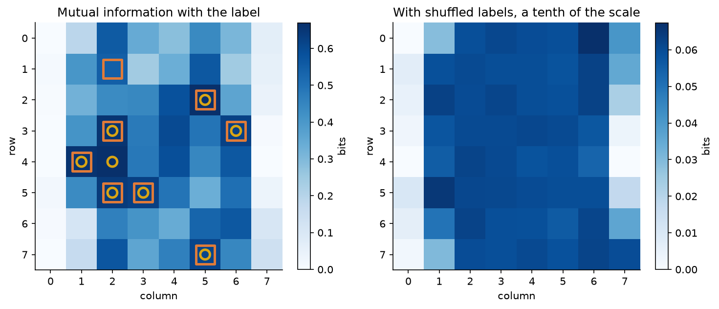
The left map shows where the information about the digit sits: in the strokes through the middle of the image, not at the edges. The markers show the two rankings agreeing on seven of their first eight pixels. The right map, on its own scale a tenth of the left one, is pure estimation bias, and its pattern follows the number of values each pixel takes rather than anything about digits.

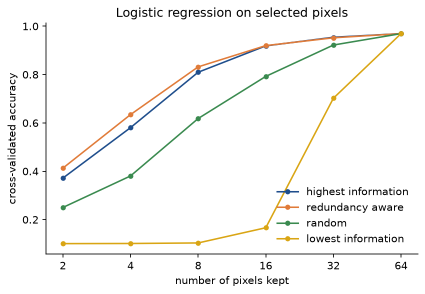
Eight well-chosen pixels already classify 81 % of the digits correctly, while eight random ones manage 62 % and the eight least informative ones barely beat the 10 % of guessing. Accounting for redundancy helps most when very few pixels are kept, about 4 to 5 points at two and four pixels and 2 points at eight, and stops mattering once sixteen pixels cover the image.

The notebook information_theory.ipynb is a guided tour in the order of this page: self-information and entropy, the riding log, the forecast, the Gaussian fits, the classifier and the sentence, the Huffman code and the ten draws, checks of every identity on random inputs, a demonstration of each pitfall, the bias simulation, the coded Markov source, the digit pixels and the library comparison. The tests in tests check the worked example value by value, the mathematical properties above and the agreement with SciPy and scikit-learn, and run in a few seconds:

python -m pytest foundations/information-theory

The handwritten digits are the test portion of the UCI Optical Recognition of Handwritten Digits data set by E. Alpaydin and C. Kaynak, licensed CC BY 4.0, which ships with scikit-learn as sklearn.datasets.load_digits, so nothing is downloaded. Everything else is defined in the code or generated from a seed.

In practice

SciPy and scikit-learn compute the same quantities, often in nats by default. Over 200 random distributions, label arrays and predicted probabilities, examples/compare_with_libraries.py finds these largest differences from the package:

• Entropy: scipy.stats.entropy(p, base=2), 9 × 10⁻¹⁶ bits; scipy.special.entr(p).sum() in nats, exactly equal.
• KL divergence: scipy.stats.entropy(p, q, base=2), 2 × 10⁻¹⁵ bits; scipy.special.rel_entr(p, q).sum() in nats, 2 × 10⁻¹⁶.
• Jensen-Shannon divergence: scipy.spatial.distance.jensenshannon(p, q, base=2) ** 2, 2 × 10⁻¹⁶.
• Mutual information of two label arrays: sklearn.metrics.mutual_info_score(x, y) in nats, 9 × 10⁻¹⁶.
• Mutual information of discrete features with a label: sklearn.feature_selection.mutual_info_classif(X, y, discrete_features=True) in nats, 6 × 10⁻¹⁶ on the 64 digit pixels.
• Log loss: sklearn.metrics.log_loss(y, probabilities) in nats, exactly equal.
• Entropy and information gain in a tree: DecisionTreeClassifier(criterion="entropy") stores node entropies in bits in tree_.impurity. A depth-one tree on the wind stores 0.9544, 0.7642 and 0.9852, and its impurity decrease is the gain, 0.0935.

import numpy as np
from scipy import stats
from sklearn.metrics import mutual_info_score

from information_theory import forecast, kl_divergence, plugin_mutual_information, riding_log

p, q = forecast()
print(stats.entropy(p, q, base=2), kl_divergence(p, q))
sky, wind, ride = riding_log()
print(mutual_info_score(sky, ride), plugin_mutual_information(sky, ride, base=np.e))

tests/test_comparisons.py asserts the agreement. In PyTorch, torch.nn.functional.cross_entropy takes logits and integer labels and returns the log loss in nats, and torch.nn.functional.kl_div(input, target) expects the log-probabilities of the model as input and the probabilities of the target as target, and computes the divergence of the model from the target, summed with reduction="sum" and averaged per example with reduction="batchmean", while the default "mean" also divides by the number of classes. PyTorch is not among this topic's dependencies, so these are not tested here.

For continuous features mutual_info_classif and mutual_info_regression do not bin the data. They use nearest-neighbour estimators (Kraskov, Stögbauer and Grassberger, and Ross for a discrete target) with a small random jitter, so they need random_state for reproducible scores and give different numbers from a histogram-based plug-in estimate.

How close do real coders get to the entropy? examples/coding_a_source.py answers on a source whose entropy rate is known exactly: a first-order Markov chain over the letters a, b, c and d. Row by row, the transition matrix gives the probabilities of the next letter after a as (0.10, 0.75, 0.10, 0.05), after b as (0.60, 0.05, 0.05, 0.30), after c as (0.30, 0.10, 0.55, 0.05) and after d as (0.85, 0.05, 0.05, 0.05). The stationary distribution is (0.3943, 0.3330, 0.1394, 0.1332), the single-letter entropy H(π) is 1.8415 bits and the entropy rate is 1.2628 bits per letter. Huffman codes for blocks of k letters, built from the exact block probabilities, cost 1.8784 bits per letter for k = 1, 1.5656 for k = 2, 1.4145 for k = 4 and 1.3384 for k = 8. They always stay within 1/k of the block entropy per letter and creep towards the rate as the theorem promises, but slowly, because the block entropy per letter is (H(π) + (k - 1) × 1.2628) / k.

On 200,000 sampled letters, with models fitted by counting on another 200,000, the bits per letter on the held-out text are:

• A fixed 2-bit code: 2.0000, perplexity 4.
• One Huffman code for single letters: 1.8799.
• The order-0 model, the letter frequencies: 1.8429, perplexity 3.5873.
• bz2 at level 9: 1.6279. zlib at level 9: 1.6143. lzma at preset 9 extreme: 1.5152.
• One Huffman code per previous letter: 1.4434.
• The order-1 model: 1.2671, perplexity 2.4067. The order-3 model: 1.2674, perplexity 2.4073.

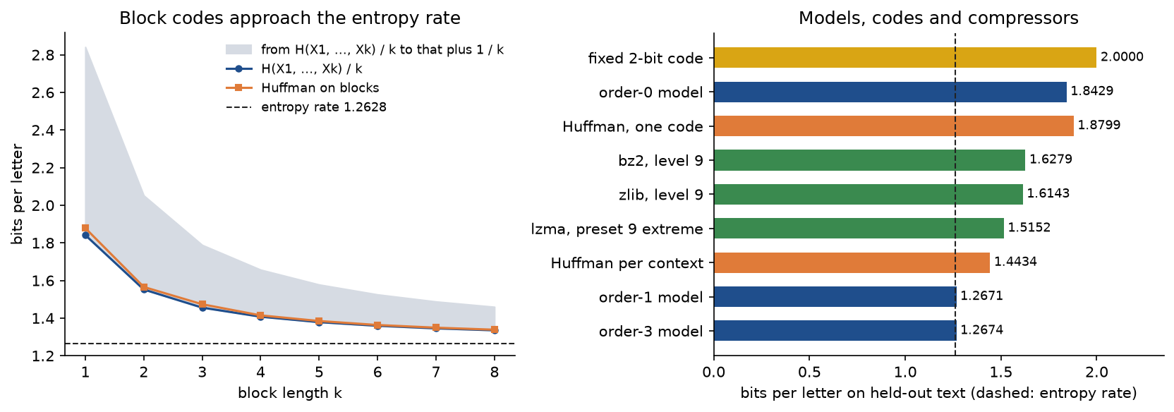
The order-1 model reaches the entropy rate up to sampling noise: the true transition matrix scores 1.2671 bits on the same text. Higher orders do not help; their training cross-entropy keeps falling, to 1.2603 bits for order 3, while their held-out cross-entropy does not, the first sign of overfitting. Huffman coding with the right model still loses 1.4434 - 1.2671 = 0.1763 bits per letter to whole-bit codewords, which arithmetic coding would recover. The general-purpose compressors find part of the structure, but none comes near the rate, because they model byte strings, not this source.

When to use which:

• Use the from-scratch functions to learn the quantities, to compute them on paper-sized examples, and when you need them in bits with explicit control over zeros and estimation.
• Use scipy.stats.entropy and scipy.special.rel_entr for entropies and divergences of known distributions, passing base=2 when you want bits, and validate inputs yourself, because SciPy normalizes them silently.
• Use mutual_info_score and mutual_info_classif(discrete_features=True) for discrete features, compare every score with a shuffled-label baseline, and keep feature selection inside cross-validation. For continuous features use the nearest-neighbour estimators with a fixed random_state rather than an arbitrary binning.
• Use log_loss or the framework's cross-entropy loss for training and evaluating classifiers, and perplexity for language models, always on held-out data and with the same tokenization when comparing models.
• Use Huffman codes when a simple and fast prefix code is enough, arithmetic or range coding when the last fraction of a bit per symbol matters, and remember that the model, not the coder, decides how close to the entropy you get.

Pitfalls

• Mixing bits and nats. scikit-learn's mutual_info_score, mutual_info_classif and log_loss report nats, scipy.stats.entropy reports nats unless given base=2, and scikit-learn's tree criterion uses bits. The riding log's mutual information is 0.2595 bits or 0.1799 nats; comparing one with the other is off by the factor ln 2 = 0.6931. examples/compare_with_libraries.py prints both.
• Reading scipy.stats.entropy(p, q) as the cross-entropy. With two arguments it returns the KL divergence, 0.1683 bits for the forecast, not the cross-entropy 1.6683. It also normalizes both arguments, so stats.entropy(p, 2 * q) returns the same 0.1683 instead of an error, and a vector of counts or of probabilities that lost a category passes silently. Similarly, scipy.spatial.distance.jensenshannon returns the Jensen-Shannon distance, 0.1950 bits for the forecast, the square root of the divergence 0.0380.
• Treating KL as a distance. It is not symmetric, 0.1683 against 0.1432 for the forecast, and the direction decides what a fit does: on the mixture, forward KL gives a broad Gaussian across both modes and reverse KL a narrow one on a single mode, with two further local minima. Say which direction you minimize and why.
• Zero probabilities. One outcome that the model rules out makes the cross-entropy, the KL divergence and the perplexity infinite: kl_divergence([0.5, 0.5], [1, 0]) is inf, and an n-gram model without smoothing gives an infinite perplexity on any sentence with an unseen bigram. scikit-learn's log_loss clips probabilities to machine precision instead, so one certain mistake adds -ln(2.2 × 10⁻¹⁶) = 36.04 nats to the sum rather than infinity, which an average over many examples can hide. Smooth models and inspect the largest per-example losses.
• Expecting conditioning to reduce entropy for every value. It does so only on average. Windy days have H(ride | windy) = 0.9852 bits, more than H(ride) = 0.9544, while H(ride | wind) = 0.8609 is less. tests/test_pitfalls.py asserts it.
• Trusting information gain on attributes with many values. An identifier column splits the data into pure single-row groups and gets the largest possible gain, 0.9544 bits on the riding log. The gain ratio divides by the split information, here log2 16 = 4, but still ranks the day number first, 0.2386 against 0.1643 for the sky, which is why C4.5 applies it only among attributes with at least average gain. The underlying cause is the plug-in bias: on 16 rows a random attribute with four values gains 0.1687 bits on average, and the first-order formula predicts 0.1353. Compare gains with a shuffled-label baseline or use held-out data.
• Rounding logarithms before combining them. Tables of log2 rounded to one decimal make each entropy wrong by up to a few hundredths of a bit, 0.9625 instead of 0.9544 for the riding decision, and gains differ by about that much. With 9 positive and 7 negative rows, the split into branches of 5 positive and 2 negative and of 4 and 5 has exact gain 0.0536, the split into 6 and 4 and 3 and 3 has exact gain 0.0069, eight times smaller, and both come out as 0.0125 with rounded logarithms. Keep at least four significant digits until the final comparison.
• Ignoring the bias of plug-in estimates. Plug-in entropy is too low and plug-in mutual information too high, by about (K - 1) / (2n) and (a - 1)(b - 1) / (2n) nats. Ten draws from a uniform variable on four values gave 1.4855 bits instead of 2; two independent variables with 8 and 4 values show 0.0612 bits of mutual information from 256 samples. Report the sample size, apply a correction or a permutation baseline, and distrust any score close to the baseline, especially for features with many values.
• Screening features one at a time or by correlation. With two fair bits and a label equal to their exclusive or, each bit has zero mutual information with the label and the pair has one full bit, so univariate ranking discards both. Correlation misses even the univariate dependence of y = x squared, which has correlation 0 and mutual information 1.5219 bits. Univariate ranking also ignores redundancy: on the digits it spends its second and third picks on the neighbouring pixels (4, 2) and (4, 1), which share 0.6184 bits, and the redundancy-aware ranking beats it by 5 points of accuracy at four pixels.
• Treating differential entropy like entropy. For a continuous variable the analogue is an integral, it can be negative and it depends on the unit, and binning it gives an entropy that grows without bound as the bins shrink:

A Gaussian with standard deviation 0.1 has differential entropy -1.2748 bits, and the same variable in units ten times smaller, standard deviation 1, has 2.0471 bits. Rounded into bins of width 0.1, 0.01 and 0.001 it has entropies 2.1048, 5.3696 and 8.6910 bits. Entropies of continuous data are only comparable at the same resolution; KL divergence and mutual information do not have this problem, because the logarithm of the bin width cancels.

• Expecting Huffman codes to reach the entropy. Codewords have whole numbers of bits, so L can be almost a full bit above H. A binary source with probabilities 0.9 and 0.1 has H = 0.4690 bits but needs 1 bit per symbol; Huffman codes for blocks of 2, 4 and 6 symbols cost 0.6450, 0.4926 and 0.4702 bits per symbol. Nor are Huffman lengths the rounded self-informations: A in the worked example has -log2 p = 1.1520 and a one-bit codeword, while the Shannon code gives it two. When checking a printed Huffman table, confirm that the Kraft sum is one and that the sum of pi ℓi reproduces the stated average.
• Comparing perplexities measured in different units. The probability 0.00125 of the example sentence is a perplexity of 3.8073 per word and 1.3969 per character over its 20 characters. Perplexities are comparable only with the same tokenization, vocabulary, treatment of unknown words and held-out text.

Every pitfall is demonstrated by examples/common_mistakes.py and in the notebook section "Pitfalls in code".

Further reading

• C. E. Shannon, "A mathematical theory of communication", Bell System Technical Journal 27, 379-423 and 623-656, 1948. Entropy, the source coding theorem and much more, in the paper that founded the field.
• T. M. Cover and J. A. Thomas, Elements of Information Theory, second edition, Wiley, 2006. Chapters 2 and 5 cover everything on this page with full proofs.
• D. J. C. MacKay, Information Theory, Inference, and Learning Algorithms, Cambridge University Press, 2003. Free online; connects coding and inference throughout.
• S. Kullback and R. A. Leibler, "On information and sufficiency", Annals of Mathematical Statistics 22(1), 79-86, 1951.
• D. A. Huffman, "A method for the construction of minimum-redundancy codes", Proceedings of the IRE 40(9), 1098-1101, 1952.
• L. G. Kraft, A device for quantizing, grouping, and coding amplitude-modulated pulses, MS thesis, Massachusetts Institute of Technology, 1949.
• B. McMillan, "Two inequalities implied by unique decipherability", IRE Transactions on Information Theory 2(4), 115-116, 1956.
• J. R. Quinlan, "Induction of decision trees", Machine Learning 1, 81-106, 1986. ID3 and information gain.
• C. M. Bishop, Pattern Recognition and Machine Learning, Springer, 2006. Section 1.6 for information theory in machine learning, section 10.1.2 for the two directions of the KL divergence.
• T. Minka, "Divergence measures and message passing", Microsoft Research technical report MSR-TR-2005-173, 2005. How the choice of divergence shapes an approximation.
• F. Jelinek, R. L. Mercer, L. R. Bahl and J. K. Baker, "Perplexity: a measure of the difficulty of speech recognition tasks", Journal of the Acoustical Society of America 62(S1), S63, 1977.
• G. A. Miller, "Note on the bias of information estimates", in H. Quastler (editor), Information Theory in Psychology: Problems and Methods, Free Press, 95-100, 1955.
• L. Paninski, "Estimation of entropy and mutual information", Neural Computation 15(6), 1191-1253, 2003.
• H. Peng, F. Long and C. Ding, "Feature selection based on mutual information: criteria of max-dependency, max-relevance, and min-redundancy", IEEE Transactions on Pattern Analysis and Machine Intelligence 27(8), 1226-1238, 2005. The redundancy-aware ranking of the sample project.
• A. Kraskov, H. Stögbauer and P. Grassberger, "Estimating mutual information", Physical Review E 69, 066138, 2004.
• B. C. Ross, "Mutual information between discrete and continuous data sets", PLoS ONE 9(2), e87357, 2014.