MNIST from scratch

Recognizing handwritten digits is the classic first real problem for a neural network: the inputs are raw pixels, the rule that separates a 4 from a 9 cannot be written down, and the data set is large enough for overfitting, initialization and optimization to matter, yet small enough to train on a laptop CPU in seconds. This page builds a complete classifier with nothing but NumPy. It downloads MNIST from a public mirror, verifies the files and parses their binary format by hand, splits the data properly, and trains a 784-100-10 network with a softmax output, the cross-entropy cost and mini-batch gradient descent with momentum, using the equations derived in Backpropagation. It then measures what each classic improvement actually buys (cross-entropy instead of squared error, a better initial scale, L2, dropout and data augmentation), reproduces overfitting on 1,000 images, looks at which digits the final network confuses, and trains the same model in PyTorch from the same initial weights until the two loss curves agree to rounding error. Afterwards you will be able to write and debug a full training pipeline yourself, from bytes on disk to a test accuracy you can trust, and you will know which tricks matter for a network of this size.

To run the code in this topic, install the base group, and the deep group for the comparison with PyTorch.

Intuition

A grey-scale image of 28 by 28 pixels is a vector of 784 numbers. The network maps it to ten numbers, one score per digit. Softmax turns the scores into probabilities, and the prediction is the digit with the highest probability. In between sits one hidden layer of 100 sigmoid units, each a learned template that responds to some combination of strokes. Training adjusts all 79,510 weights and biases so that the probability of the correct digit goes up on the training images.

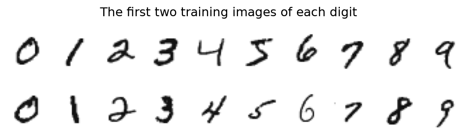
The samples show how much the same digit varies: slant, stroke width, open or closed loops. MNIST stores the strokes as bright values on a dark background; the figures on this page draw them as ink on paper.

Everything else on this page is about making that training reliable:

• The data must be read correctly and split so that the final number means something. Settings are chosen on a validation set carved out of the training images, and the test set is touched once.
• The cost decides how strongly a wrong answer pulls on the weights. Squared error behind a softmax barely moves an output that is confidently wrong; cross-entropy pulls hardest exactly there.
• The initial weights decide whether the hidden units start in the useful middle of the sigmoid or in its flat tails, where the gradient is almost zero.
• Momentum averages successive gradients, so steps along a consistent direction grow and zig-zags cancel.
• A network with 79,510 parameters can memorize thousands of images. L2 keeps the weights small, dropout stops units from relying on each other, and augmentation shows the network slightly rotated and shifted digits it has never seen. Which of these actually helps is an empirical question, answered under In practice.

The diagram shows the whole model. Solid blue arrows are the forward pass and dashed orange arrows the backward pass. Compared with the network in Backpropagation, three things are new: the softmax output, which turns the output error into the simple difference A2 - Y; the dropout mask, which the error passes back through; and the L2 penalty, which adds λW to every weight gradient.

The pipeline is the order of this page. Everything above the dashed box happens once; the box runs once per mini-batch, 782 times per epoch; the validation set is measured after every epoch, and the test set only once, after every choice has been made.

How it works

Notation

The notation is the one of Backpropagation. The network has L layers of weights; here L = 2, with 784 inputs, 100 hidden units and 10 outputs. For each layer l:

• The weight matrix W has one row per unit of layer l and one column per unit of layer l - 1, and its entry in row j and column k is the weight to unit j from unit k. This is the layout of torch.nn.Linear.weight.
• The bias vector b has one entry per unit, the net inputs z = W a + b hold one value per unit, and the activations apply the layer's activation function to them. The hidden layer uses the sigmoid σ, the output layer softmax. The net inputs of the output layer are also called logits.
• The error δ of a unit is the derivative of the cost with respect to its net input.
• A mini-batch of m examples is stored one example per row: X holds the images, Y the one-hot targets, with a 1 in the column of the true digit c and 0 elsewhere, and Z, A and Δ hold the net inputs, activations and errors of a layer, one row per example.
• The symbol ⊙ multiplies entry by entry. The other symbols are the L2 strength λ, the dropout rate p with its mask R, the learning rate η, the momentum coefficient μ and the velocity v.

The formula images write the layer as a superscript in parentheses. In the text, W1, b1, Z1, A1, Δ1 and R1 are short for the weights, biases, net inputs, activations, errors and dropout mask of layer 1, and likewise for layer 2. In mini-batch form, the four backpropagation equations B1 to B4 read

where row i of G is the gradient of example i's cost with respect to the outputs and the bold 1 is a column of m ones. Three parts of this page change them: a softmax output, which does not act entry by entry, changes B1; dropout changes B2; and L2 changes B4.

The data and its file format

MNIST holds 70,000 grey-scale images of handwritten digits, 60,000 for training and 10,000 for testing, each 28 by 28 pixels with values from 0 (background) to 255 (ink). The digits were scaled to fit a 20 by 20 box and centred by their centre of mass. The writers of the training images and those of the test images are different people, so the test set measures how well the network reads handwriting it has never seen.

The files use the IDX format, which is simple enough to parse by hand. A file starts with a four-byte magic number: two zero bytes, a type code and the number of dimensions d. The type codes are 0x08 for unsigned bytes, 0x09 for signed bytes, 0x0B for 16-bit integers, 0x0C for 32-bit integers, 0x0D for 32-bit floats and 0x0E for 64-bit floats. Then come d sizes, each a 32-bit unsigned integer stored most significant byte first (big-endian), and finally the values in row-major order, also big-endian. The label files have one dimension and one byte per image.

The diagram decodes the header of the training images byte by byte; the worked example below does the hexadecimal arithmetic. A file is consistent when its length equals the header length plus the number of values times the bytes per value:

Here s is the size of one value in bytes. parse_idx checks this before reading anything, which catches a truncated or padded file at once.

Preprocessing divides every pixel by 255. This is a fixed transformation with nothing estimated from the data, so it cannot leak information between the sets. Had we standardized each pixel with a mean and a standard deviation, those statistics would have to come from the fitting images alone (Data leakage and pitfalls).

Three disjoint sets play three roles. 50,000 training images are used for fitting, the other 10,000 training images form the validation set on which every setting is chosen, and the 10,000 test images are evaluated once, at the end. The split is stratified: within each digit, a fixed share of the images goes to validation, so both parts keep the class proportions to within 0.00006. A random validation split shares writers with the fitting set, unlike the test set, so it can be slightly optimistic; on this page the two agree to within a few hundredths of a percentage point.

Softmax and cross-entropy

The output layer turns the logits z into probabilities:

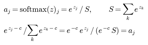
The outputs are positive and add up to one, and raising one logit lowers every other output. The second line shows that adding the same constant to every logit changes nothing. Implementations therefore subtract the largest logit first, so the largest exponential is e⁰ = 1 and nothing can overflow.

The cost of one example whose true digit is c is the negative log-probability of that digit, the cross-entropy between the one-hot target and the output:

The last form, a log-sum-exp, is how it is computed: it never forms the probability of the true digit, which could round to zero and make the logarithm infinite.

B1 needs the derivative of the cost with respect to the logits. Because every softmax output depends on every logit, the derivative goes through the full matrix of derivatives J, the Jacobian:

The bracket [k = j] is 1 when k = j and 0 otherwise. The chain rule sums over all outputs, and for cross-entropy the derivative of the cost with respect to output k is minus y over a:

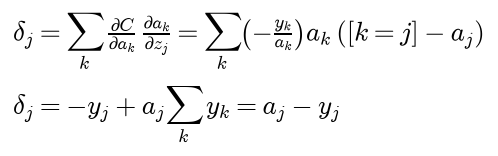
The last step uses the fact that the one-hot target sums to one. In mini-batch form, B1 for softmax with cross-entropy is a subtraction:

The same cancellation happens for a sigmoid output with binary cross-entropy in Backpropagation; Loss functions treats it in general.

For comparison, the squared error, one half of the squared distance between output and target, has gradient g = a - y with respect to the outputs, and the Jacobian gives

Every entry carries a factor of its own output, and the bracket is small when one output dominates. An output that is confidently wrong therefore produces almost no error signal. For three outputs with logits (4, 0, -4) when the true class is the third one, the outputs are (0.9817, 0.0180, 0.0003). The cross-entropy error is (0.9817, 0.0180, -0.9997) with length 1.4012, the squared-error error (0.0177, -0.0170, -0.0006) with length 0.0245, 57 times smaller.

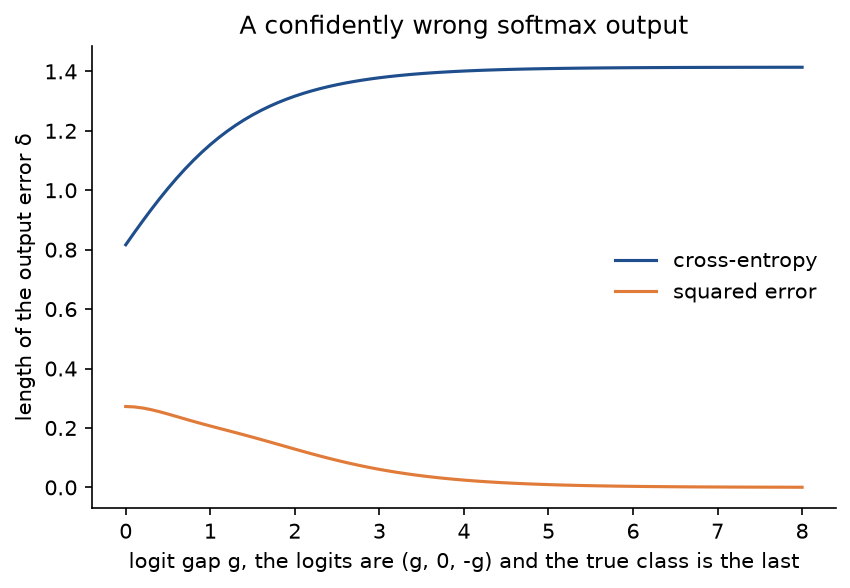
The plot repeats the comparison for growing gaps. The more confidently wrong the network is, the harder cross-entropy pulls, approaching the square root of 2, while the squared error lets go. This is the learning slowdown that cross-entropy removes.

Initialization

With zero biases and independent zero-mean weights of standard deviation s, a hidden net input of one image is a sum of 784 independent terms, so its variance is the sum of their variances:

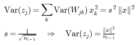
An MNIST image has about 150 non-zero pixels and a squared length of 87.87 on average. With s = 1 the net inputs have a standard deviation near √87.87 = 9.374 (9.565 measured on 1,000 images), and 62.1 % of them have σ'(z) < 0.01, against a maximum of 0.25: the sigmoid units start saturated and B2 multiplies their errors by almost zero. Scaling by the fan-in, s = 1/√784 = 1/28, gives a standard deviation near 9.374 / 28 = 0.335 (0.342 measured), the steep middle of the sigmoid, and no saturated units at all. This is the rule initialize_network uses by default, with an extra factor √2 for ReLU layers; Activations and initialization derives the Xavier and He variants.

L2 regularization

L2 adds the squared size of every weight to the cost of the mini-batch:

Only B4 changes, by the derivative of the penalty:

Biases are not penalized: they shift a unit's threshold without making the function steeper, and penalizing them only biases the fit. The second line shows why L2 is also called weight decay: with plain gradient descent, every step first shrinks the weights by the factor 1 - ηλ, where C0 is the cost without the penalty. Some texts scale the penalty by the training-set size n, as λ' / (2n) times the sum of squared weights; that is the same thing with λ = λ' / n. Regularization compares L2 with L1 and early stopping.

Dropout

During training, each hidden unit is switched off with probability p, independently for every example and for every mini-batch. Inverted dropout scales the survivors up by 1 / (1 - p):

Since every entry of the mask has expected value 1, the expected activation equals the activation without dropout, so the network is evaluated with every unit present and nothing rescaled. For example, with p = 0.5 the activations (0.6, 0.2, 0.9, 0.4) and the keep pattern (1, 0, 1, 0) give (1.2, 0, 1.8, 0).

The next layer reads the masked activations, so B4 for layer l + 1 uses them in place of the plain ones. In B2, the error that reaches the activation function passes back through the same mask:

A dropped unit receives no error, and its incoming weights get no gradient from that example. Training therefore averages over many thinned networks that share weights, which discourages units that are useful only in combination with particular others.

Momentum

Gradient descent with momentum keeps one velocity per parameter, initially zero, and for every mini-batch gradient g updates

This is the form PyTorch's torch.optim.SGD uses, which matters for comparing the two exactly. Unrolled, the velocity is a geometrically weighted sum of all past gradients:

When the gradient keeps pointing the same way, the velocity approaches g / (1 - μ), so with μ = 0.9 the effective step is ten times η; components that change sign from batch to batch cancel. With L2, g includes the λW term, exactly as PyTorch's weight_decay adds it before the momentum step. Optimizers compares momentum with RMSProp and Adam.

Data augmentation by rotation and shift

Each fitting image in a mini-batch is rotated by a random angle θ drawn uniformly between -10 and 10 degrees and shifted by random offsets drawn uniformly between -2 and 2 pixels in each direction, freshly for every epoch. The warp is computed backwards: for every output pixel at row r and column c, find the source position it comes from and interpolate there, so every output pixel gets exactly one value. With the image centre (r0, c0) at row and column 13.5 and the shift (tr, tc), a counterclockwise rotation reads from

The source position is generally not a pixel centre. Bilinear interpolation mixes the four surrounding pixels, each weighted by how close the source position lies to it:

Pixels outside the image count as background, 0. A shift by whole pixels and a rotation by 90 degrees reproduce exact copies, which the tests check against slicing and np.rot90.

The training loop

For each epoch, the fitting images are shuffled with a seeded generator and cut into mini-batches of 64. For each mini-batch:

1. Augment the images if augmentation is on, and draw fresh dropout masks if dropout is on.
2. Run the forward pass:

1. Compute the output error by B1 for softmax, the hidden error by B2 with the mask, and the gradients by B3 and by B4 with the λW term.
2. Update every parameter with momentum.

After each epoch the network is evaluated without dropout or augmentation on the fitting set and on the validation set, recording the mean cross-entropy and the accuracy. The test set is evaluated once, after all choices have been made.

Worked example

A network small enough to follow by hand: three inputs (a three-pixel image), two sigmoid hidden units and three softmax outputs. The cost is cross-entropy plus an L2 penalty with λ = 0.1, the learning rate is η = 0.5 and the momentum μ = 0.9.

The diagram gives every parameter. As matrices, W1 has the rows (0.5, -0.4, 0.3) and (-0.2, 0.6, -0.5), one row per hidden unit; b1 is (0.1, -0.1); W2 has the rows (0.7, -0.3), (-0.6, 0.4) and (0.2, 0.9); and b2 is (0.0, 0.1, -0.1). The mini-batch holds two images, the rows (0.0, 0.5, 1.0) and (1.0, 0.5, 0.0) of X, of classes 2 and 0 (counting from 0), so the rows of Y are (0, 0, 1) and (1, 0, 0).

Every value is computed in double precision and shown to four decimals. Sums written out from rounded terms can differ from these in the last digit, as noted where it happens.

Reading an IDX header by hand

Before the network, the data. The first sixteen bytes of the training-image file are 00 00 08 03 00 00 ea 60 00 00 00 1c 00 00 00 1c. Bytes 2 and 3 say unsigned bytes and three dimensions. The first size, 00 00 ea 60 read most significant byte first, is 14 × 16³ + 10 × 16² + 6 × 16 + 0 = 57,344 + 2,560 + 96 = 60,000 images, and 00 00 00 1c is 1 × 16 + 12 = 28 rows and again 28 columns. The pixels start at byte 4 + 4 × 3 = 16.

Forward pass

Each hidden net input is a row of W1 times the image plus the bias. For image 1 and hidden unit 1 that is 0.5 × 0.0 - 0.4 × 0.5 + 0.3 × 1.0 + 0.1 = 0.2. Applying the sigmoid and then the output layer gives:

• Image 1: hidden net inputs (0.2, -0.3), hidden activations (0.5498, 0.4256), logits (0.2572, -0.0597, 0.3930).
• Image 2: hidden net inputs (0.4, 0.0), hidden activations (0.5987, 0.5000), logits (0.2691, -0.0592, 0.4697).

The softmax of the first row by hand: subtract the largest logit, 0.3930, to get (-0.1358, -0.4526, 0); exponentiate to (0.8731, 0.6359, 1), which sum to 2.5090; divide by the sum. The output probabilities are:

• Image 1: (0.3480, 0.2535, 0.3986).
• Image 2: (0.3399, 0.2448, 0.4154).

The network gives the correct class probability 0.3986 for image 1 (class 2) but only 0.3399 for image 2 (class 0). The per-example costs are -ln 0.3986 = 0.9199 and -ln 0.3399 = 1.0792, and their mean is 0.9995. Averaging the two rounded costs gives 0.99955 instead, exactly halfway between two four-decimal values; the exact mean, 0.999548, lies just below the midpoint. The squared weights of W1 add up to 1.15 and those of W2 to 1.95, so the penalty is 0.1 / 2 × (1.15 + 1.95) = 0.1550, and the cost is C = 0.9995 + 0.1550 = 1.1545.

Backward pass

B1 for softmax with cross-entropy is a subtraction, the outputs minus the targets:

• Image 1: output errors (0.3480, 0.2535, -0.6014).
• Image 2: output errors (-0.6601, 0.2448, 0.4154).

Each row sums to zero, because both the outputs and the targets add up to one in every row; the rounded entries shown sum to 0.0001. B2 sends the errors back along the weights, which multiplies each row by W2, and multiplies entry by entry by the sigmoid derivatives σ'(z) = a(1 - a):

• Image 1: sent back (-0.0288, -0.5443), hidden derivatives (0.2475, 0.2445), hidden errors (-0.0071, -0.1331).
• Image 2: sent back (-0.5259, 0.6698), hidden derivatives (0.2403, 0.2500), hidden errors (-0.1263, 0.1674).

For image 1 and hidden unit 2, 0.3480 × (-0.3) + 0.2535 × 0.4 - 0.6014 × 0.9 = -0.5443, and times 0.2445 that gives -0.1331.

Gradients with the L2 term

B4 averages the outer products over the two images and adds λW; B3 averages the errors.

• The data part of the output weight gradient, one half of the transposed output errors times A1, has the rows (-0.1019, -0.0910), (0.1429, 0.1151) and (-0.0410, -0.0241).
• Adding 0.1 W2 gives the gradient of W2, with the rows (-0.0319, -0.1210), (0.0829, 0.1551) and (-0.0210, 0.0659), and the gradient of b2 is (-0.1561, 0.2491, -0.0930).
• The gradient of W1 has the rows (-0.0132, -0.0734, 0.0264) and (0.0637, 0.0686, -0.1165), and the gradient of b1 is (-0.0667, 0.0172).

The top-left entry is 1/2 × (0.3480 × 0.5498 - 0.6601 × 0.5987) + 0.1 × 0.7 = -0.1019 + 0.07 = -0.0319. The output-bias gradients sum to zero, like the rows of the output errors: raising every logit by the same amount changes nothing, so the output biases can only learn differences.

Update with momentum

The velocities start at zero, so after the first mini-batch each velocity equals its gradient and the step is plain gradient descent, every parameter minus 0.5 times its gradient:

• W1 becomes the rows (0.5066, -0.3633, 0.2868) and (-0.2319, 0.5657, -0.4417), and b1 becomes (0.1334, -0.1086).
• W2 becomes the rows (0.7160, -0.2395), (-0.6415, 0.3224) and (0.2105, 0.8671), and b2 becomes (0.0780, -0.0246, -0.0535).

The cost on the same mini-batch falls from 1.1545 to 1.0734, 0.9273 for the data plus 0.1461 for the penalty.

Momentum shows up in the second step. Repeating the forward and backward pass with the new parameters gives the output-bias gradient (-0.1171, 0.2020, -0.0849). The velocity becomes 0.9 × (-0.1561, 0.2491, -0.0930) + (-0.1171, 0.2020, -0.0849) = (-0.2576, 0.4262, -0.1686), about twice the new gradient, and the output biases move to (0.0780, -0.0246, -0.0535) - 0.5 × (-0.2576, 0.4262, -0.1686) = (0.2068, -0.2376, 0.0308). The middle entry is -0.2377 from the rounded terms and -0.2376 at full precision. Every other parameter is updated the same way. After two steps the cost is 0.9703; two steps of plain gradient descent would reach only 1.0188.

A central-difference gradient check on this network, penalty included, gives a relative error of 3.3 × 10⁻¹⁰. Every number in this section is asserted by tests/test_trace.py and printed by examples/worked_step.py.

The code

The package mnist_from_scratch is NumPy and the standard library, split into one module per idea. PyTorch is imported only inside the functions of comparisons.py, so everything else works without it.

• arrays.py holds the array types and the number of classes.
• idx.py reads and writes the IDX format: parse_idx_header, parse_idx, encode_idx and read_idx for gzip files.
• download.py holds the mirrors and pinned SHA-256 sums, fetch, which downloads one file and keeps it only if its checksum matches, and load_mnist, which returns the four arrays.
• preparation.py holds stratified_split, to_features, one_hot and prepare_splits, which returns the fitting, validation and test sets in one Splits value.
• activations.py holds the sigmoid and ReLU with their derivatives, and losses.py softmax, log-softmax, the Jacobian, both costs and output_delta, B1 for either cost.
• propagation.py is the heart of the topic: forward_pass with optional dropout masks and backward_pass, B2 to B4 with the mask and the L2 term.
• network.py holds the frozen DigitNetwork class, which works in single or double precision, and initialize_network with the fan-in or unit scale.
• regularization.py holds the L2 penalty and dropout_masks, momentum.py the velocity and momentum_step, and augmentation.py warp, random_warp and augment_features.
• training.py holds TrainingSettings, train, which returns the trained network and a History, evaluate and batch_orders.
• trace.py holds worked_example, trace_step, which keeps every value of one step, and format_trace, which prints them.
• gradient_check.py checks the backward pass against central differences, over every parameter of a small network or over a random sample of parameters of the full one.
• experiments.py holds the configurations of the experiments under In practice and the runners run_overfitting and run_improvements, so the examples and the notebook share them.
• evaluation.py holds the confusion matrix, the recall of every digit and the most frequent confusions, and pitfalls.py the measurements behind the Pitfalls section.
• images.py reads a digit from an image file and prepares it the way MNIST prepared its digits, and checkpoints.py saves and loads a trained network.
• comparisons.py copies networks to and from PyTorch, computes autograd gradients and trains with torch.optim.SGD.
• plotting.py and digit_plots.py draw every figure in the handbook's four colours and save it reproducibly.

Python counts from zero, so weights[0] is W1, and forward.activations[l] is the activation of layer l with the dropout mask applied, starting with the inputs. The backward pass in propagation.py is the mini-batch form of B2 to B4 with the two changes derived above, the mask in B2 and the λW term in B4:

for layer in range(len(weights) - 1, 0, -1):
    propagated = delta @ weights[layer]
    mask = forward.masks[layer - 1]
    if mask is not None:
        propagated = propagated * mask
    delta = propagated * derivative(forward.pre_activations[layer - 1])
    deltas.append(delta)
deltas.reverse()
weight_gradients = tuple(
    d.T @ a / count + l2 * w for d, a, w in zip(deltas, forward.activations[:-1], weights)
)
bias_gradients = tuple(d.sum(axis=0) / count for d in deltas)

A complete training run of the final classifier takes a few lines:

from mnist_from_scratch import CLASSIFIER, initialize_network, load_mnist, prepare_splits, train

splits = prepare_splits(load_mnist())
validation = (splits.validation_inputs, splits.validation_labels)
start = initialize_network((784, 100, 10))
network, history = train(start, splits.fit_inputs, splits.fit_labels, CLASSIFIER, validation)

train is deterministic: the batch order comes from batch_orders(seed), and the augmentation angles and dropout masks from a second generator seeded from the same seed, so the PyTorch comparison can replay the same batches. MNIST runs in single precision, which halves the time of every matrix product; the gradient checks and the PyTorch agreement run in double precision.

The examples and the project import the package, so install the repository first as described in the main README. The examples each demonstrate one idea and run from the repository root:

• examples/worked_step.py decodes the IDX header, prints every value of the worked example in the order above, both steps, the softmax by hand, and the gradient checks of all eight configurations of hidden activation, cost and depth with L2 and dropout masks.
• examples/explore_data.py downloads and verifies MNIST, prints the shapes, class counts and split statistics, measures the initial net inputs under both scales and saves the samples figure.
• examples/common_mistakes.py demonstrates the mistakes listed under Pitfalls and saves the figure of output-error sizes and the rotated 6.
• examples/overfitting.py runs the experiment on 1,000 images and saves its figure, in 15 to 30 seconds.
• examples/compare_improvements.py trains the eight configurations compared under In practice and saves their figure, in 30 to 50 seconds.
• examples/compare_with_pytorch.py compares gradients and a full training run with PyTorch, shows the extra-softmax mistake and times inference.

python neural-networks/mnist-from-scratch/examples/worked_step.py
python neural-networks/mnist-from-scratch/examples/explore_data.py
python neural-networks/mnist-from-scratch/examples/common_mistakes.py
python neural-networks/mnist-from-scratch/examples/overfitting.py
python neural-networks/mnist-from-scratch/examples/compare_improvements.py
python neural-networks/mnist-from-scratch/examples/compare_with_pytorch.py

The sample project, project/mnist_classifier.py, is a command-line digit classifier. By default it verifies or downloads MNIST, splits off the validation set, checks the gradients of the full network on 60 randomly chosen parameters, and trains the configuration that wins the comparison under In practice: cross-entropy, fan-in initialization and augmentation by rotations of up to 10 degrees and shifts of up to 2 pixels, retrained on all 50,000 fitting images for 12 epochs with batches of 64, learning rate 0.1 and momentum 0.9. It then evaluates the test set once, prints the recall of every digit and the most frequent confusions, saves three figures and stores the trained network in .data/mnist-from-scratch/classifier.npz. Options such as --hidden, --activation, --epochs, --l2, --dropout, --max-angle and --seed change the setup, and --figures sends the PNGs to another folder so a custom run does not overwrite the ones shown here. The default run takes 13 to 20 seconds on one laptop CPU thread, depending on what else the machine is doing.

python neural-networks/mnist-from-scratch/project/mnist_classifier.py
python neural-networks/mnist-from-scratch/project/mnist_classifier.py --export-test-image 0 seven.png
python neural-networks/mnist-from-scratch/project/mnist_classifier.py --classify seven.png

With --classify, the project labels image files with the stored network and prints the three most likely digits. An image must be 28 by 28 pixels or a whole multiple of that, such as a 280 by 280 drawing, which is averaged down. A digit drawn dark on light paper is recognized by its bright border and inverted, and the ink is moved so that its centre of mass sits where MNIST puts it, at row and column 14: the network only understands images prepared the way its training images were. --export-test-image writes a test image as a PNG to try this on; test image 0, a 7, comes back as a 7 with probability 0.9998.

With the defaults, the network reaches 98.08 % on the unaugmented fitting images and 97.80 % on validation after the last epoch. The test set, evaluated once, gives an accuracy of 0.9783 and a cross-entropy of 0.0659, that is 217 errors among 10,000 images written by people the network has never seen. The validation accuracy predicted the test accuracy to within 0.03 points.

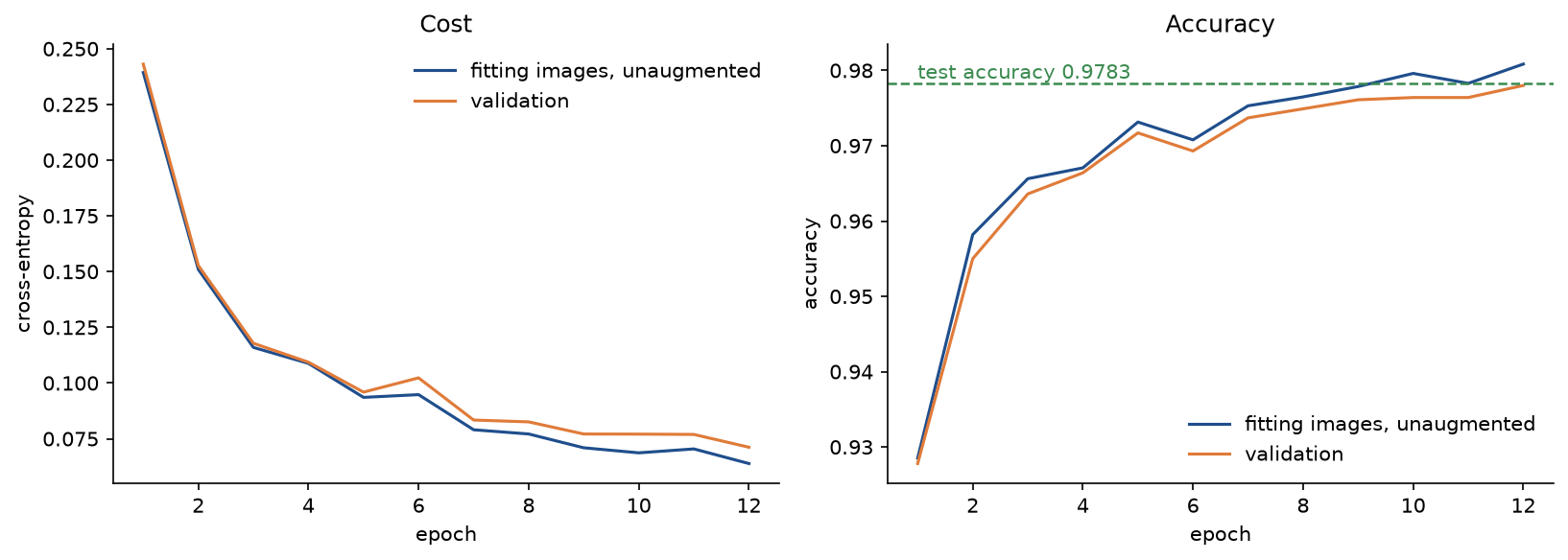
The fitting and validation curves stay close together: with augmentation and 50,000 images, this network is limited by its capacity and its training time, not by overfitting. Validation accuracy is still creeping up at the end, with the zig-zag that a constant learning rate and mini-batch noise produce. More epochs with a decaying learning rate, a wider or deeper network, or a convolutional network (Convolutional networks) are the next steps.

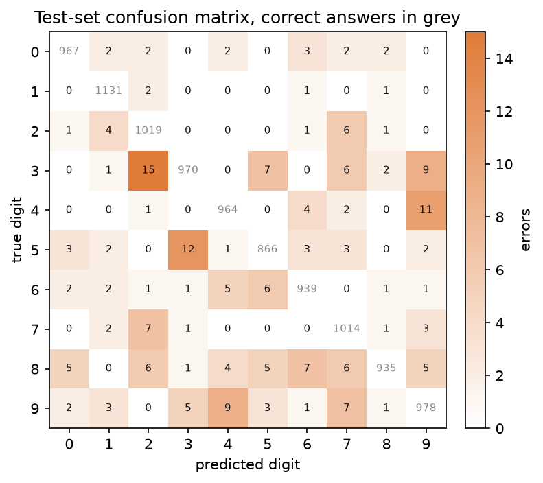
Recall per digit ranges from 99.65 % for 1 down to 96.04 % for 3 and 96.00 % for 8. The most frequent confusions are 3 read as 2 (15 times, never the other way round), 5 read as 3 (12 times, and 3 as 5 7 times), 4 read as 9 (11 times, and 9 as 4 9 times) and 3 read as 9 (9 times). The pairs share strokes: an open 3 whose lower bowl is flattened looks like a 2, a 5 with a closed top looks like a 3, and a 4 with a closed top looks like a 9.

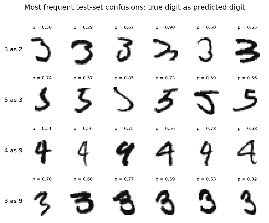
Many of the misread digits are ones a person reads at once, and the network often gives the wrong digit a probability near one half: a sign that the decision is close, not that the image is ambiguous. A dense network sees each image as an unordered list of 784 numbers and has no notion that a stroke shifted by one pixel is the same stroke, which is what convolutional networks add. Evaluation metrics covers per-class precision and recall in general.

The notebook mnist_from_scratch.ipynb is a guided tour in the order of this page: the worked example through trace_step and again in bare NumPy, gradient checks, the IDX format on a tiny array, loading and splitting MNIST, each pitfall, the overfitting experiment, the comparison of improvements, the final classifier with its errors and an image file classified, and the same model in PyTorch. It takes one to two minutes on one CPU thread. The tests in tests check the worked example value by value, the IDX parser and the checksum verification, the mathematical properties above and the agreement with PyTorch, and run in a few seconds:

python -m pytest neural-networks/mnist-from-scratch

Data: MNIST by Yann LeCun, Corinna Cortes and Christopher J. C. Burges, built from two databases of handwriting collected by the US National Institute of Standards and Technology. LeCun and Cortes hold the copyright and make the data set available under the Creative Commons Attribution-Share Alike 3.0 licence. fetch downloads the four gzip files, about 11 MB, on first use from the mirror torchvision uses (ossci-datasets.s3.amazonaws.com/mnist), falling back to the one TensorFlow Datasets uses (storage.googleapis.com/cvdf-datasets/mnist); both serve byte-identical files whose MD5 sums match the ones torchvision publishes. Each file is checked against the SHA-256 sum pinned in MNIST_SHA256 before it is moved into .data/mnist-from-scratch/ at the repository root, and the IDX header and file length are validated before any array is read. Nothing is committed.

In practice

The numbers in this section come from the example scripts, run on one thread for NumPy and for PyTorch. Results are reproducible to the last digit with the same thread count and processor; another thread count or processor sums floating-point numbers in a different order and can change them slightly.

Overfitting on 1,000 images

examples/overfitting.py trains the 784-100-10 network with cross-entropy and fan-in initialization on 1,000 fitting images for 150 epochs, in batches of 20 with learning rate 0.05 and momentum 0.9, and evaluates the full validation set after every epoch. It runs three times:

• Without regularization, every fitting image is classified correctly from epoch 20. The validation cost is lowest at epoch 8, 0.4156, and ends at 0.6004. Validation accuracy peaks at 0.8789 in epoch 11 and ends at 0.8781.
• With L2, λ = 10⁻³, the fitting images are all right from epoch 33. The validation cost is lowest at epoch 15, 0.4123, and ends at 0.4169. Validation accuracy peaks at 0.8808 and ends at 0.8780.
• With augmentation by rotations of up to 10 degrees and shifts of up to 2 pixels, the fitting images are all right only from epoch 91. The validation cost keeps falling to 0.1647 at epoch 148 and ends at 0.1786. Validation accuracy peaks at 0.9513 and ends at 0.9488.

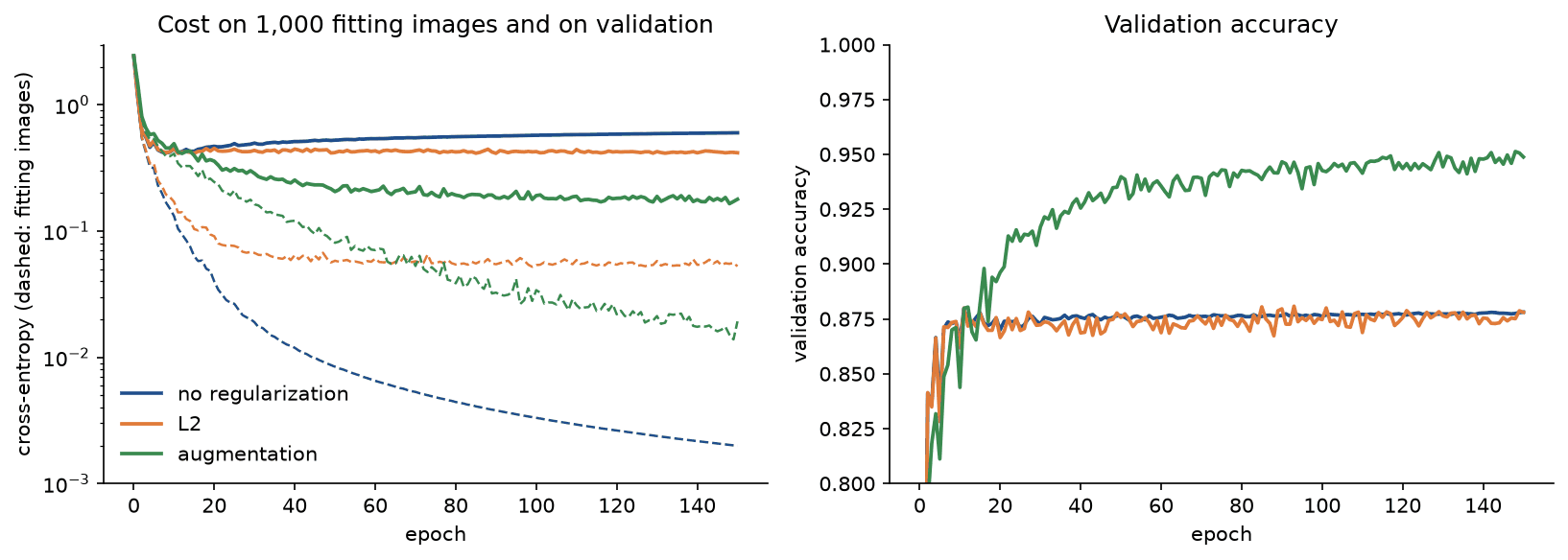
Without regularization the network memorizes the 1,000 images by epoch 20 and its fitting cost keeps falling towards zero, while the validation cost bottoms out at epoch 8 and then climbs by 44 %. Validation accuracy ends only 0.08 points below its peak: the network hardly gets more answers wrong, it gets its wrong answers more confidently wrong, which only the cost reveals. L2 holds the validation cost near its minimum but leaves the accuracy where it was. Augmentation changes the picture: with a new random rotation and shift of every image in every epoch there are effectively far more than 1,000 images, the validation cost keeps falling almost to the end of the run, and the accuracy ends near 95 %, seven points higher.

What each improvement buys

examples/compare_improvements.py trains eight configurations on a 10,000-image fitting subset, 30 epochs each with batches of 64, learning rate 0.1 and momentum 0.9 and the same seed, so every run starts from the same random draw (rescaled for the fan-in initialization) and sees the same batches. For each it reports the fitting accuracy, the validation accuracy and the validation cost after the last epoch, and the change in validation accuracy against the cross-entropy network with fan-in initialization:

• Squared error with N(0, 1) initialization: fitting 0.8622, validation 0.8057, cost 1.8326, change -0.1493.
• Cross-entropy with N(0, 1) initialization: fitting 0.9972, validation 0.9132, cost 0.3476, change -0.0418.
• Squared error with fan-in initialization: fitting 0.9712, validation 0.9338, cost 0.2444, change -0.0212.
• Cross-entropy with fan-in initialization, the reference: fitting 0.9995, validation 0.9550, cost 0.1622.
• Plus L2 with λ = 10⁻⁴: fitting 0.9985, validation 0.9547, cost 0.1538, change -0.0003.
• Plus dropout with p = 0.2: fitting 0.9961, validation 0.9567, cost 0.1500, change +0.0017.
• Plus augmentation by 10 degrees and 2 pixels: fitting 0.9833, validation 0.9724, cost 0.0892, change +0.0174.
• Plus all three: fitting 0.9746, validation 0.9695, cost 0.1120, change +0.0145.

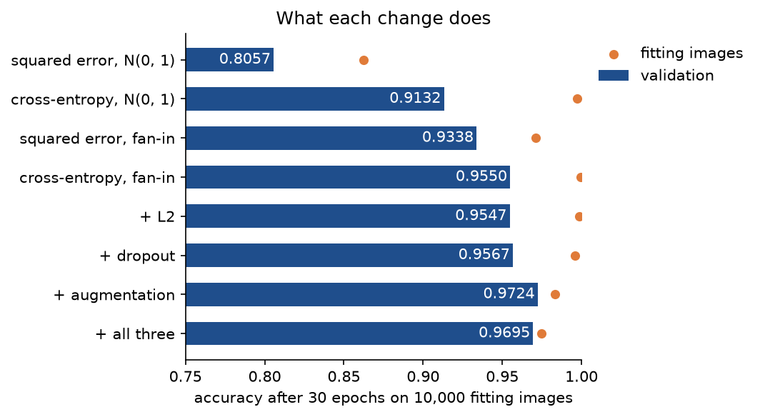
What the comparison says:

• Cross-entropy and the initial scale are the two large effects, and they compound. With N(0, 1) weights, switching from squared error to cross-entropy is worth 10.8 points; with fan-in weights it is still worth 2.1 points, because softmax outputs saturate during training even when the hidden units do not. The fan-in scale is worth 12.8 points with squared error and 4.2 points with cross-entropy. The classic baseline, squared error with N(0, 1) weights, cannot even fit its own training images (86.2 %).
• L2 and dropout barely change the accuracy of a 100-unit network on 10,000 images, but both lower the validation cost, from 0.1622 to 0.1538 and 0.1500: they make the network less overconfident. Their value grows with the size of the network relative to the data.
• Augmentation is the only regularizer that adds information, and it is worth 1.7 points on its own.
• The benefits do not add up. All three together are worse than augmentation alone, because each regularizer slows fitting, and after 30 epochs the combination fits only 97.5 % of its own training images. Every regularizer has to earn its place on the validation set, with enough epochs to let it.

The project retrains the winner, augmentation alone, on all 50,000 fitting images. Regularization and Loss functions go deeper into the individual effects.

The same model in PyTorch

The same network and training loop in PyTorch is torch.nn.Sequential, CrossEntropyLoss applied to the logits, and torch.optim.SGD with momentum, using two parameter groups so that weight decay, our L2 term, applies to the weights and not to the biases. The core of train_torch in comparisons.py:

model = to_torch(network, settings.dropout)
named = list(model.named_parameters())
groups = [
    {"params": [p for n, p in named if n.endswith("weight")], "weight_decay": settings.l2},
    {"params": [p for n, p in named if n.endswith("bias")], "weight_decay": 0.0},
]
optimizer = torch.optim.SGD(groups, lr=settings.learning_rate, momentum=settings.momentum)
criterion = torch.nn.CrossEntropyLoss()
for order in batch_orders(len(targets), settings.epochs, settings.seed):
    model.train()
    for start in range(0, len(order), settings.batch_size):
        batch = torch.from_numpy(order[start : start + settings.batch_size])
        optimizer.zero_grad()
        criterion(model(features[batch]), targets[batch]).backward()
        optimizer.step()

examples/compare_with_pytorch.py first checks the gradients: on random networks with one and two hidden layers, cross-entropy and an L2 term, autograd and our backward pass agree to within 6 × 10⁻¹⁷. Then it trains both from the NumPy network's initial weights on the same batches in the same order, in double precision, with L2 (λ = 10⁻⁴) and without dropout or augmentation. Two epochs over all 50,000 fitting images give the costs 0.2213 and 0.1541 in both implementations. The largest difference between the two cost curves is 6 × 10⁻¹⁷, and the largest difference between any two weights after 1,564 updates is 2 × 10⁻¹⁵: the two compute the same function and the same gradients and differ only in the order of floating-point additions. test_momentum_training_matches_pytorch_sgd and test_gradients_match_autograd in tests/test_comparisons.py assert the agreement on small problems.

With dropout on, the two draw different random masks, so the runs agree only statistically. torchvision, which is not in the dependency groups, offers the remaining pieces: torchvision.datasets.MNIST downloads the same four files from the same mirror and checks their MD5 sums, and transforms.RandomAffine(degrees=10, translate=(2 / 28, 2 / 28)) performs a similar augmentation, with nearest-neighbour interpolation unless bilinear is requested.

Inference speed

The example also times the trained network in single precision on one thread, as two matrix products in NumPy and as the PyTorch model, predicting all 10,000 test images at once and one image at a time. Both give the same predicted digit for every test image, and their logits differ by at most 4 × 10⁻⁶, the size of single-precision rounding error for logits of this magnitude. On our laptop a batch of 10,000 images takes about 1.5 to 1.8 microseconds per image in either framework, and one image per call about 7 microseconds in NumPy and 10 to 11 in PyTorch; the exact timings change from run to run.

For a large batch, both spend nearly all their time in the same kind of single-precision matrix product, and they finish within a few per cent of each other; which one is ahead changes from run to run. One image per call costs several times more per image than a batch, because fixed costs per call and a less efficient matrix-vector product dominate; those fixed costs are larger in PyTorch, whose dispatcher handles autograd, devices and data types for every module it calls.

When to use which

• Write the network by hand to understand it: every gradient, the masks of dropout and the bookkeeping of momentum are visible and testable, as in the worked example.
• Use PyTorch, or another framework with automatic differentiation, for anything beyond a fixed small architecture: new layers need no backward pass, the same code runs on a GPU, and data loading, augmentation and mixed precision come ready-made.
• For deploying a small trained network on a CPU, a few lines of NumPy, or a compact runtime, are as fast as the framework and have far fewer dependencies.

Pitfalls

• Squared error behind a softmax. Its output error carries a factor of the output itself, so a confidently wrong network hardly learns: for logits (4, 0, -4) with the third class true, the error is 57 times smaller than with cross-entropy, and in the comparison above squared error costs 2.1 to 10.8 points of validation accuracy. examples/common_mistakes.py prints the numbers and draws the curves shown under How it works.
• Unscaled pixels. Feeding raw values 0 to 255 makes every hidden net input 255 times larger: at the start, 95.7 % of the hidden net inputs have σ'(z) < 0.01, and after one epoch on 10,000 images the network reaches 34.67 % validation accuracy instead of 87.84 %. This run is chaotic enough that another processor can land a few points away; the collapse itself is robust. Scale the inputs, and if you standardize them, estimate the statistics on the fitting set only. examples/common_mistakes.py and the notebook section "Unscaled pixels" show it.
• Initializing with unit variance. N(0, 1) weights with 784 inputs give hidden net inputs with a standard deviation near 9.4 and saturate most sigmoid units before training starts, which costs 4.2 points of validation accuracy even with cross-entropy. Scale by the fan-in.
• Computing softmax and its logarithm naively. np.exp(z) / np.exp(z).sum() returns nan for a logit of 1,000, and np.log(softmax(z)) returns -inf when a probability rounds to zero. Subtract the maximum before exponentiating and compute the cross-entropy from the logits with log-sum-exp, as softmax and cross_entropy do (notebook section "Softmax without the shift").
• Applying softmax before CrossEntropyLoss. PyTorch's CrossEntropyLoss and F.cross_entropy expect logits and apply log-softmax themselves. Given probabilities, they apply softmax twice, so even a perfect prediction, probability 1 for the right digit and 0 for the nine others, is scored as the softmax of those ten numbers:

The cost can never fall below 1.4612, and the gradient reaching the logits shrinks, on 256 validation images from length 0.0199 to 0.0069 in examples/compare_with_pytorch.py. Its relative nn.NLLLoss expects log-probabilities, not probabilities. - Reading IDX in the wrong byte order. IDX stores integers big-endian. np.frombuffer(data, dtype=np.uint32) uses the machine's byte order, little-endian on x86 and ARM, and reads the image count 00 00 ea 60 as 1,625,948,160 instead of 60,000; use int.from_bytes(..., "big") or the type ">u4". Check the header and the file length before trusting any array (test_reading_the_header_as_little_endian_gives_nonsense). - Choosing anything on the test set. Picking the number of epochs, λ, the dropout rate or the architecture by test accuracy turns the test set into a second validation set, and its accuracy becomes an optimistic estimate. Every choice on this page is made on the validation split, and the test set is evaluated once (Data leakage and pitfalls measures how large the optimism gets). - Dropout done wrong. Three common mistakes: leaving dropout on at evaluation, which drops the validation accuracy of a network trained for two epochs with p = 0.5 from 90.33 % to between 85.86 % and 86.29 %, depending on the random masks (examples/common_mistakes.py); drawing one mask per epoch instead of a fresh mask for every mini-batch, which trains one fixed thinned network instead of averaging many; and halving the weights at evaluation when the training code already divided by 1 - p, which scales the activations twice. Original dropout multiplies by the keep probability at evaluation, inverted dropout does it during training; use one, not both. - Augmentations that change the label or leak. A rotation of a few degrees keeps the digit; a rotation by 180 degrees turns a 6 into a 9 and teaches the network a wrong label. Augment only the fitting data, after the split, and never the validation or test images.

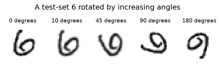
At 10 degrees the digit is unmistakably the same; at 180 it is a different digit, which is why the augmentation here stops at 10 degrees.

• Watching only accuracy. In the overfitting experiment, the validation cost rises by 44 % between epoch 8 and epoch 150 while the validation accuracy ends 0.08 points below its best: the network is becoming confidently wrong. Track the validation cost as well, and stop or regularize when it turns upwards.
• Stacking every regularizer. L2, dropout and augmentation each slow fitting, and their benefits do not add up. Together they scored 0.29 points below augmentation alone in the comparison above. Add one at a time and keep each only if the validation set says so.
• Mixing conventions for L2 and momentum. A penalty written as λ' / (2n) times the sum of squared weights, with n the training-set size, corresponds to λ = λ' / n here, so the same λ' means a much stronger penalty on 1,000 images than on 50,000. Penalizing the biases as well, which PyTorch's weight_decay does unless the parameters are split into groups, changes the model slightly. And momentum μ = 0.9 multiplies the effective learning rate by ten, so a learning rate tuned for plain gradient descent can diverge once momentum is switched on.
• Classifying an image prepared differently from the training data. A digit photographed or drawn as dark ink on white paper, off centre or at another size, looks nothing like an MNIST digit to the network. read_digit_image inverts, averages down and centres such images, as the project's --classify option shows; it does not rescale the digit to the 20 by 20 box MNIST uses, so a very small or very large drawing can still be misread.

Further reading

• Y. LeCun, L. Bottou, Y. Bengio and P. Haffner, "Gradient-based learning applied to document recognition", Proceedings of the IEEE 86(11), 2278-2324, 1998. Introduces MNIST and compares dense and convolutional networks on it.
• M. A. Nielsen, Neural Networks and Deep Learning, chapters 1 and 3, 2015. A free online book that builds a sigmoid network for MNIST and improves it step by step.
• X. Glorot and Y. Bengio, "Understanding the difficulty of training deep feedforward neural networks", AISTATS 2010. Why the initial scale must depend on the fan-in.
• A. Krogh and J. A. Hertz, "A simple weight decay can improve generalization", Advances in Neural Information Processing Systems 4, 1991.
• N. Srivastava, G. Hinton, A. Krizhevsky, I. Sutskever and R. Salakhutdinov, "Dropout: a simple way to prevent neural networks from overfitting", Journal of Machine Learning Research 15, 1929-1958, 2014.
• B. T. Polyak, "Some methods of speeding up the convergence of iteration methods", USSR Computational Mathematics and Mathematical Physics 4(5), 1-17, 1964. The heavy-ball method behind momentum.
• I. Sutskever, J. Martens, G. Dahl and G. Hinton, "On the importance of initialization and momentum in deep learning", ICML 2013.
• P. Y. Simard, D. Steinkraus and J. C. Platt, "Best practices for convolutional neural networks applied to visual document analysis", ICDAR 2003. Affine and elastic distortions of MNIST digits as augmentation, for dense and convolutional networks.
• I. Goodfellow, Y. Bengio and A. Courville, Deep Learning, chapters 6 to 8, 2016. Softmax outputs, regularization and optimization in depth.