Evaluation metrics

A classifier outputs a score, a decision needs a threshold, and a single number is supposed to say how good the result is. Which number is not a detail. Accuracy rewards a fraud model that never flags anything, a weighted F1 score hides a class the model never predicts, a ROC curve can rank two models in the opposite order from the precision-recall curve, a well-ranked model can produce probabilities that are useless for setting a threshold, and a cross-validated score without an interval cannot separate two models that differ by noise. This page builds the confusion matrix and every common measure derived from it, derives why the area under the ROC curve is the probability that a random positive outranks a random negative, shows why precision-recall curves are the more informative view under heavy imbalance, chooses a threshold from the costs of the two errors, measures calibration, covers the regression metrics, and ends with cross-validation and bootstrap confidence intervals. Twelve scored units are worked through by hand, everything is implemented from scratch in NumPy and checked against scikit-learn, and a sample project writes a complete evaluation report for a screening task. Afterwards you will be able to pick the metric that answers your actual question, compute it by hand, spot the averaging and imbalance traps, and report a result with an honest uncertainty. It builds on Probability and statistics and evaluates the models of Logistic regression and Naive Bayes.

To run the code in this topic, install the base group, and the ml group for the breast-cancer data of the sample project and the comparisons with scikit-learn and SciPy.

Intuition

An evaluation asks questions of a model's output on data it has not seen. The output comes in three strengths, and each supports different questions.

• Decisions at one threshold. Flag or do not flag. The four counts of the confusion matrix (true and false positives, false and true negatives) answer questions such as "of the units we flagged, how many were faulty?" (precision) and "of the faulty units, how many did we catch?" (recall). Each answer conditions on something different, which is why one number never tells the whole story.
• A ranking. Most models output a score, and every threshold gives a different confusion matrix. Sweeping the threshold traces the ROC curve (catch rate against false-alarm rate) and the precision-recall curve. Their areas summarize how well the scores rank positives above negatives, wherever the threshold is eventually put.
• Probabilities. If a score of 0.8 should mean "80 % of such cases are positive", the scores are calibrated, and only then can a threshold be computed from the costs of the two kinds of error instead of being searched for.

Two more questions sit around every metric: where the scores came from (cross-validation or a held-out test set, so that every score is a prediction on data the model did not fit) and how much the number would move on a different sample (the bootstrap).

The map follows the page. The three branches below the scores are the three strengths of output, the amber arrows show where costs and calibration decide the threshold, and the green node at the bottom is the last step of every honest evaluation: an interval around the number.

The imbalance problem runs through all of it. When positives are rare, almost every number that mixes the two classes is dominated by the negatives: accuracy becomes the true negative rate, and the ROC curve spends most of its area on false-alarm rates no one would ever operate at. The measures that survive imbalance either condition on the positives (precision, recall, the precision-recall curve) or correct for chance (balanced accuracy, the Matthews correlation, Cohen's kappa).

How it works

Notation

The evaluation data hold n examples. Example i has a true label y, equal to 1 for the positive class and 0 for the negative class, and a score s, larger meaning more likely positive. A threshold t turns scores into decisions: the prediction is 1 when s is at least t. At a given threshold, TP, FP, FN and TN count the true positives, false positives, false negatives and true negatives. P = TP + FN is the number of positives, N = FP + TN the number of negatives, and the prevalence π = P / n is the share of positives. With K classes, the confusion matrix entry C with indices j and k counts the examples of true class j predicted as class k. A predicted probability is written p, the cost of one false positive cFP and of one false negative cFN, and Φ is the distribution function of the standard normal distribution. The formula images write the same quantities with subscripts, such as c with the subscript FP; the text writes them plainly.

The confusion matrix

For two classes the confusion matrix has one row per true class and one column per predicted class.

The green diagonal holds the correct decisions and the orange cells the two kinds of error. This is scikit-learn's layout, rows actual and columns predicted, with the negative class first, so confusion_matrix(y, y_hat).ravel() returns TN, FP, FN, TP in that order. Many texts transpose it or put the positive class first; always check the labels before reading a matrix.

With K classes, the diagonal of the K by K matrix holds the correct predictions. Treating class k as positive and every other class as negative gives one-versus-rest counts:

A false positive for class k is an error in column k, a false negative an error in row k. Every error is a false negative for its true class and a false positive for the class it was mistaken for, so the false positives summed over all classes and the false negatives summed over all classes both equal the number of errors, a fact used below.

Rates and the questions they answer

The rates divide one count by a total:

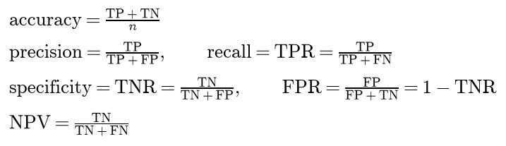
Each answers one question and is blind to something:

• Accuracy asks what share of predictions is right, and ignores which class the errors fall into.
• Precision, also called the positive predictive value, asks what share of the flagged examples is positive, and ignores the positives that were missed.
• Recall, also called sensitivity or the true positive rate, asks what share of the positives is flagged, and ignores false alarms.
• Specificity, the true negative rate, asks what share of the negatives is left alone, and ignores missed positives. The false positive rate is its complement.
• The negative predictive value asks what share of the examples left alone is negative, and ignores false alarms.

Recall and specificity condition on the truth: each is computed within one true class, so neither depends on how many examples the other class has. Precision and the negative predictive value condition on the prediction, and they do depend on the class balance. A rate whose denominator is zero, for example precision when nothing is flagged, is undefined; scikit-learn returns 0 with a warning by default (its zero_division option), and so does the package.

F1 and F-beta

Precision and recall pull against each other: flagging more examples raises recall and usually lowers precision. The F1 score combines them by the harmonic mean, and substituting the definitions shows that it is a simple ratio of counts:

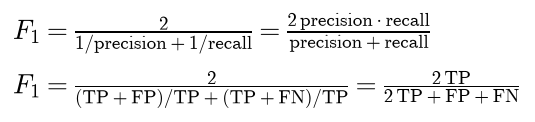
The harmonic mean is pulled towards the smaller of the two numbers: precision 1 and recall 0.01 give an arithmetic mean of 0.505 but an F1 of only 0.0198. A model cannot score well by being excellent at one and useless at the other.

When one error matters more, weight the reciprocals, with weight β² / (1 + β²) on recall and 1 / (1 + β²) on precision:

A false negative costs β² times as much as a false positive in the denominator. F2 favours recall, F0.5 favours precision, and F-beta tends to recall as β grows and to precision as β shrinks. In van Rijsbergen's original reading, β is the ratio of recall to precision at which the user is indifferent to trading one for the other. Every F score ignores the true negatives entirely, which suits retrieval, where the pile of irrelevant documents is uninteresting, and misleads when correct rejections matter.

Averaging over classes

With K classes, compute a measure M (precision, recall or an F score) for each class against the rest and average. The support of class k is the number of examples that truly belong to it.

Macro averaging weighs every class equally, weighted averaging every class by its support, and micro averaging every example equally. Three identities follow from the definitions and are worth knowing, because they make some reported numbers redundant:

• Micro precision, micro recall and micro F1 all equal accuracy when each example has exactly one true and one predicted class. Pooled, the true positives count the correct predictions, and the false positives and the false negatives both count the errors, so all three equal correct / (correct + errors).
• Weighted recall is accuracy, because the supports cancel:

Reporting weighted recall next to accuracy therefore adds nothing.

• Macro recall is the balanced accuracy, the mean of the per-class recalls.

Each average misleads in its own way. Micro and weighted averages are dominated by the large classes, so a model that never predicts a rare class loses almost nothing; macro averaging exposes it. Macro averaging gives a class with five examples the same weight as one with five hundred, so it is noisy, and one undefined per-class score (set to 0 by zero_division) moves it a lot. And "macro F1" has two definitions in the literature: the mean of the per-class F1 scores, which scikit-learn computes, and the F1 of the macro precision and the macro recall, which is never smaller and can be noticeably larger. State which one you report.

Imbalance and chance-corrected measures

Splitting the correct predictions by class shows what accuracy really weighs:

Accuracy weights the two class-wise rates by the class shares. A classifier that never flags anything has a true positive rate of 0 and a true negative rate of 1, hence accuracy 1 - π: 0.99 when 1 % of the examples are positive. This is the accuracy paradox: under heavy imbalance, accuracy mostly measures the true negative rate, and a useless model beats a useful one. Balanced accuracy removes the weights and gives every constant classifier 0.5.

Precision depends on the prevalence even when the model does not change. Writing TP as TPR times πn and FP as FPR times (1 - π)n is Bayes' rule:

A model with a true positive rate of 0.8413 and a false positive rate of 0.1587 has precision 0.8413 at π = 0.5, 0.3708 at π = 0.1 and 0.0508 at π = 0.01. The same model, the same threshold: at 1 % prevalence nineteen of every twenty alarms are false.

The Matthews correlation coefficient (MCC) is Pearson's correlation between the label vector and the prediction vector, both coded 0 and 1. The covariance of the two vectors simplifies to a difference of products of counts, and the variance of a 0 and 1 vector is the product of its two counts over n²:

It lies between -1 and 1, is 0 for any constant prediction (the denominator is zero and the value is defined as 0), uses all four counts and is symmetric in the two classes: swapping which class is called positive leaves it unchanged, unlike precision, recall and F1. For K classes, with c correct predictions and the row totals t and column totals p of each class, the same correlation generalizes to

which reduces to the two-class formula for K = 2.

Cohen's kappa compares the observed agreement with the agreement expected if the predictions were drawn independently of the truth with the same marginal frequencies:

Kappa is 1 for perfect agreement, 0 for agreement at chance level and negative below it. For ordered classes, weighted kappa charges a disagreement by its distance, linearly or quadratically, against the counts expected by chance:

With weight 1 for every disagreement this is the unweighted kappa again. Both MCC and kappa still depend on the prevalence, so compare them only between models evaluated on the same data.

Thresholds and the ROC curve

Every threshold gives one confusion matrix and one point (FPR, TPR). At an infinite threshold nothing is flagged and the point is (0, 0); at a threshold below every score everything is flagged and the point is (1, 1). Sort the scores in decreasing order and lower the threshold past them one distinct value at a time: a positive moves the point up by 1/P, a negative moves it right by 1/N, and a group of tied scores containing a positives and b negatives moves it diagonally, b/N to the right and a/P up, in a single step, because no threshold can separate tied examples. The resulting staircase is the ROC curve.

Two invariances follow directly. The curve depends only on the order of the scores, so any strictly increasing transformation (a logarithm, a sigmoid, a recalibration) leaves it unchanged. And the true positive rate is computed within the positives and the false positive rate within the negatives, so duplicating every negative, or changing the prevalence in any other way that keeps each class's score distribution, leaves it unchanged too. The ROC curve describes the ranking, not any particular decision and not the class balance. A random ranking follows the diagonal; a perfect ranking passes through (0, 1).

The area under the ROC curve as a probability

Let S+ be the score of a positive and S- the score of a negative, each drawn uniformly from the evaluation data. The area under the ROC curve (AUC) is the probability that the positive scores higher, counting ties as one half:

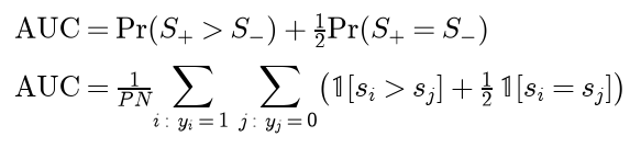
The proof reads the area off the staircase, one negative at a time. The curve moves right only when the threshold passes negatives. A negative that is not tied with any positive adds a horizontal step of width 1/N, and the height of the curve during that step is the share of positives already passed, those scoring above it; the step contributes 1/N times that share, which is its number of correctly ordered pairs divided by PN. A tied group with a positives and b negatives, entered at height h, adds a trapezoid of width b/N whose sides have heights h and h + a/P. Its area splits evenly among the b negatives:

Each tied negative gets 1/N times h + a/(2P). Here hP counts the positives scored above it and a those tied with it, so each tied pair contributes one half. Summing over all negatives gives the double sum.

The AUC is therefore the probability that the model ranks a randomly chosen positive above a randomly chosen negative, and it equals the Mann-Whitney U statistic divided by PN. Rank all n scores from 1 upwards, giving tied scores the mean of the ranks they span, and let R+ be the sum of the positives' ranks. The rank of a positive is 1 plus the number of scores below it plus half the number of other scores tied with it. Summed over the positives, the comparisons among positives contribute exactly P(P - 1)/2, one for each pair, and the ones contribute P, so

which computes the AUC with a single sort. Two consequences are used later. First, a model that outputs only hard 0 or 1 predictions has a ROC "curve" with a single corner at (FPR, TPR), and its area is

which is the balanced accuracy, not a property of any ranking. Second, for binormal scores, negatives from the standard normal distribution and positives from a normal distribution with mean d and standard deviation σ, the difference S+ - S- is normal with mean d and variance 1 + σ², so the AUC and, for σ = 1, the whole curve are known exactly:

The imbalance study below uses these exact values to check its estimates.

Precision-recall curves and average precision

The precision-recall curve plots precision against recall over all thresholds. Recall moves only when a positive is passed; precision rises after each positive and falls after each negative, so the curve is a sawtooth, not a monotone staircase. At an infinite threshold precision is 0/0; scikit-learn's convention places that point at precision 1 and recall 0.

Average precision (AP) summarizes the curve as a step function. With the thresholds in decreasing order:

Only thresholds at which recall rises contribute, each with the precision reached there. Without ties, recall rises by 1/P at the rank of each positive, so AP is the mean, over the positives, of the precision among the examples ranked at or above it. A random ranking has an expected precision of π at every recall, so its AP is about π: the baseline of a precision-recall plot is the prevalence, not 0.5.

AP is not the trapezoidal area under the plotted points. Between two thresholds no classifier can achieve the precisions on the straight line joining them: interpolating between two operating points means flagging a random share of the extra examples, which mixes their counts linearly, and precision is a ratio of counts, so the achievable curve between the points is not a straight line in precision-recall space. On a fine curve the trapezoid rule usually lands a little below AP because it averages across the sawtooth; on a coarse curve with few distinct scores, and with the conventional starting point at precision 1, it can be far above it.

Why precision-recall curves matter under heavy imbalance

The precision formula above contains the ratio of the false positive rate to the prevalence. Precision of one half or better needs

At π = 0.01 every operating point worth having lies at a false positive rate below about 0.01, the leftmost one percent of the ROC plot. The AUC averages the true positive rate uniformly over all false positive rates from 0 to 1, so 99 % of its weight sits where the application will never operate, and two models can have almost the same AUC, or the AUC can even favour the wrong one, while differing completely where it matters. The precision-recall curve plots exactly the quantity that the region near a false positive rate of zero controls, so it separates such models. The ROC curve keeps its own advantage: it is independent of the prevalence, which makes it the right tool for comparing models across data sets with different class balance, while a precision-recall curve is only meaningful at the prevalence of the data it was computed on and must be recomputed, for example with the precision formula, for a different deployment rate.

Choosing a threshold by cost

Suppose the model's probability p is calibrated, so a fraction p of the examples with that score are positive. Flagging such an example costs cFP when it turns out negative, an expected cFP (1 - p); not flagging costs cFN when it is positive, an expected cFN p. Flagging is the cheaper decision exactly when

The default threshold 0.5 is the special case of equal costs. With a missed positive ten times as expensive as a false alarm, the threshold is 1/11 = 0.0909. In ROC terms, the expected cost per example is linear in the two rates, so the points of equal cost lie on straight lines of slope m:

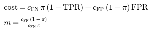
The cheapest operating point is where the highest such line touches the ROC curve. For m = 1 that maximizes TPR - FPR, Youden's index.

The formula for the threshold holds only for calibrated probabilities, and only at the prevalence they were calibrated for. For scores that are not calibrated, choose the threshold that minimizes the total cost cFP FP(t) + cFN FN(t) on validation data, out-of-fold predictions for instance, and never on the test set, whose score would then be optimistic.

Calibration

A model is calibrated if, among the examples it gives probability 0.3, 30 % are positive, and likewise for every other value:

A reliability diagram checks this by grouping the predictions into bins of predicted probability and plotting, for each non-empty bin, the mean prediction against the observed share of positives; a calibrated model lies on the diagonal. The expected calibration error (ECE) summarizes the diagram as the gaps between the points and the diagonal, weighted by the share of predictions in each bin:

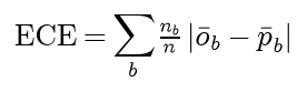
Its value depends on the number and placement of the bins (equal widths or equal counts) and on which bin a value on an edge belongs to; scikit-learn's calibration_curve closes the bins on the right, so 0.5 belongs to the bin below it.

The Brier score is the mean squared error of the probabilities:

It is a proper scoring rule: if the true probability of an example is q, the expected score of forecasting p is smallest at p = q, so honest probabilities are rewarded.

Murphy's decomposition separates two properties. Group the examples by their distinct forecast values, and for each group take its forecast f, its size and its observed share of positives o; let ō be the overall share of positives:

Reliability is the calibration error (smaller is better), resolution measures how far the forecasts separate groups with different outcome rates (larger is better), and uncertainty is the Brier score of always forecasting the base rate ō, the reference a useful model must beat. The identity follows by expanding each squared error around its group's observed share, where the cross term sums to zero within each group, and splitting the remaining spread around ō in the same way.

Calibration and ranking are separate properties. A strictly increasing map changes the probabilities but not the ROC curve, so a model can have an excellent AUC and useless probabilities. Platt scaling repairs calibration by fitting a one-feature logistic regression to held-out scores s:

Isotonic regression fits any monotone map instead and needs more data. Both must be fitted on data the model was not trained on, or they learn the model's overconfidence on its own training set. Log loss is the other common proper score; Loss functions treats it.

Regression metrics

For targets y and predictions ŷ with errors e = ŷ - y:

RMSE and MAE are in the units of the target. Since the mean of squares is at least the square of the mean, RMSE is at least MAE, with equality only when every absolute error is the same; a large gap signals a few large errors. A useful way to see what each metric rewards is to ask which constant forecast c minimizes it. The derivative of the summed squared error is zero at the mean, so MSE prefers the mean. The derivative of the summed absolute error is the number of targets below c minus the number above, zero at the median, so MAE prefers the median. For positive targets the percentage error behaves differently:

It crosses zero at the median weighted by 1/y. Small targets get large weights, so MAPE prefers forecasts below the median: it rewards under-forecasting. The same asymmetry shows in its range. For non-negative forecasts an under-forecast can cost at most 100 % (forecasting 0), while an over-forecast has no limit (forecasting three times the target costs 200 %). MAPE is undefined when a target is zero and explodes when targets are near zero; scikit-learn divides by the larger of the absolute target and the machine epsilon, about 2.2 × 10⁻¹⁶, so a single zero target produces a value of order 10¹⁵ instead of an error.

R² compares the squared error with that of forecasting the mean of the evaluation targets themselves. It is 1 for a perfect model, 0 for that constant, and negative for a model worse than it, which happens routinely on test data: the evaluation set's own mean is a forecast no model was given. The denominator is the spread of the actual values around their mean, not of the predictions. R² equals the squared correlation between targets and predictions only for a least-squares fit with an intercept, evaluated on the data it was fitted to.

Cross-validation

k-fold cross-validation splits the rows into k folds, fits on k - 1 of them and predicts the held-out one, so every row receives exactly one out-of-fold prediction. There are then two ways to turn those predictions into one number.

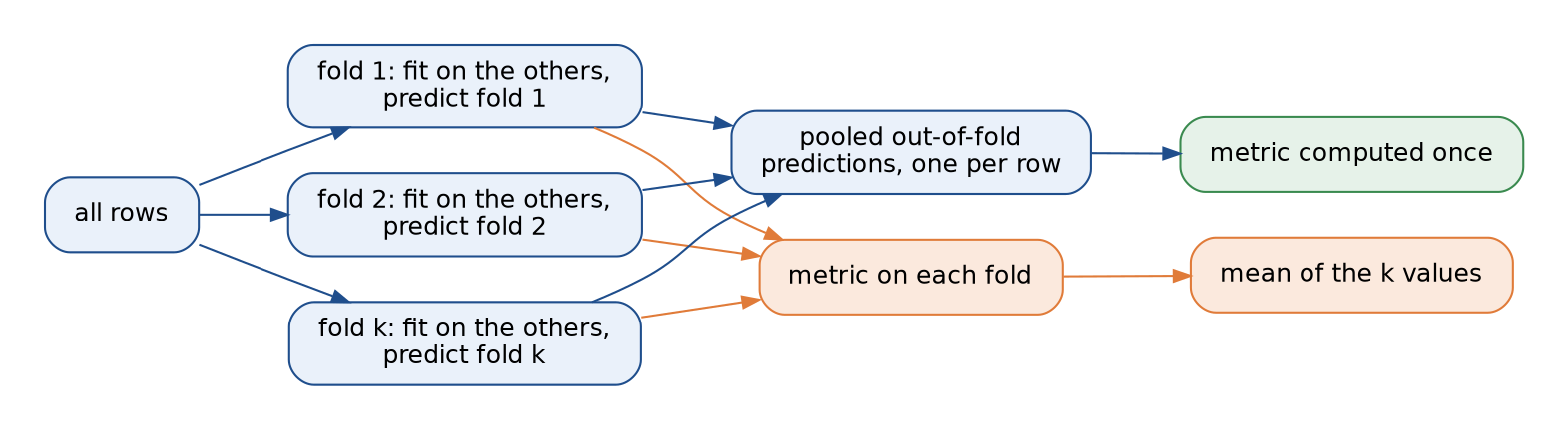
The two routes agree for accuracy and other means of per-row terms when the folds have equal sizes, but not for ratios or nonlinear functions. Precision, F1 and AUC computed per fold and averaged differ from their pooled values, and for RMSE the concavity of the square root makes the fold average optimistic for folds of equal size:

Pooling has its own condition: it treats the scores of different folds, which come from different fitted models, as one ranking, and that is only fair if the models put their scores on the same scale.

The splitters differ in which rows may share a fold:

• Plain k-fold cuts the rows, optionally shuffled, into k consecutive blocks. With rare positives some folds may receive none, and their recall is undefined. For 10 positives among 200 rows, a fold of 20 rows receives none of them with probability

so about a third of such folds have no positive at all.

• Stratified k-fold keeps each class's share the same in every fold. scikit-learn's version sorts the labels, deals them round-robin to the folds to fix how many examples of each class each fold receives, and then assigns each class's examples to folds in blocks, shuffled if asked. Fold class counts then differ by at most one.
• Grouped k-fold keeps every row of a group (a patient, a speaker, a household) in one fold, so that a model is always tested on groups it has not seen. scikit-learn places the groups from the largest to the smallest, each into the fold with the fewest rows so far.
• Time-series splitting trains on everything before a test block and tests on the block, optionally leaving a gap of rows in between, so the model never sees the future.

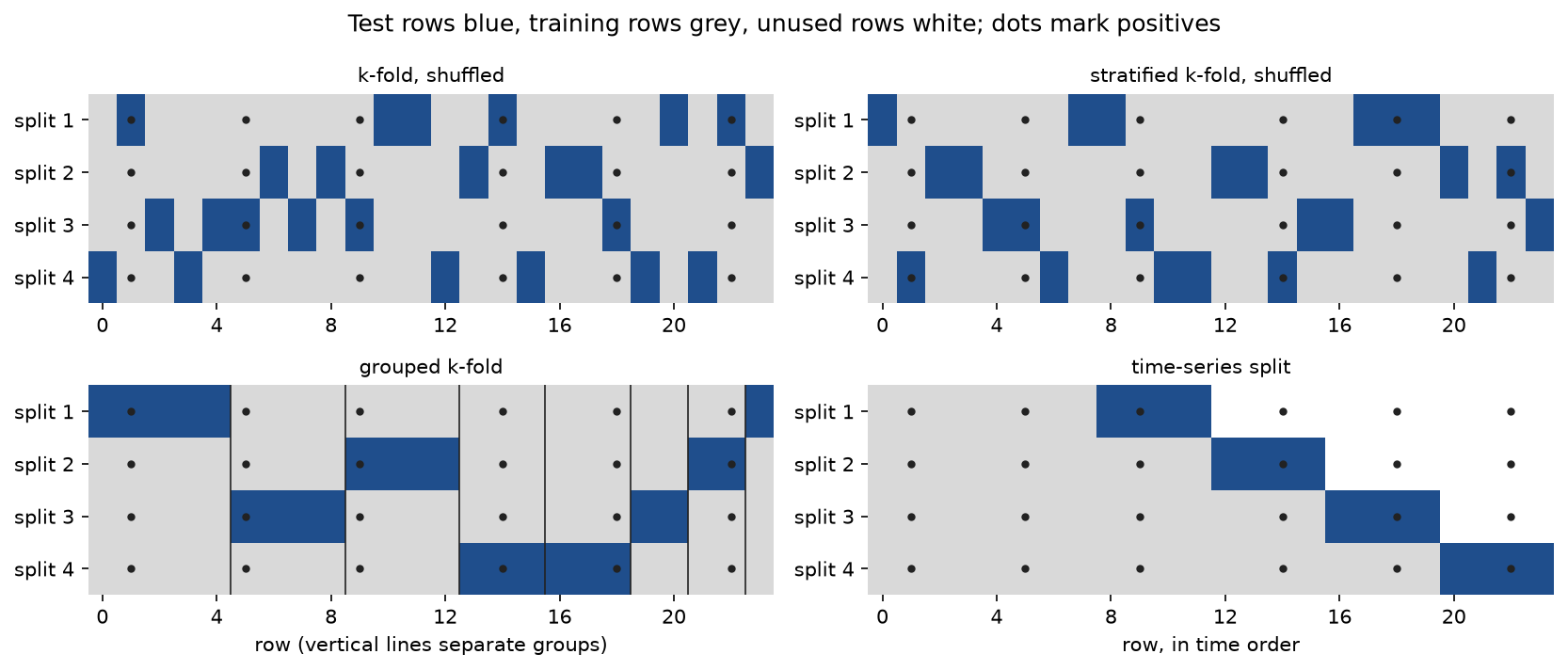
The figure shows the four splitters on 24 rows with six positives and eight groups of unequal size, drawn by examples/folds_and_intervals.py. Shuffled plain k-fold puts 3, 0, 3 and 0 positives in its four test folds, the stratified folds hold 1, 1, 2 and 2, grouped k-fold balances the groups into four test folds of six rows each, and every time-series split trains only on rows before its test block.

Which splitter is required is a question about how data arrive in use, and choosing the wrong one leaks information into the score; Data leakage and pitfalls demonstrates each case. For the uncertainty of a cross-validated score, note that the fold scores are not independent, because the training sets overlap: no unbiased estimator of the variance of k-fold cross-validation exists, and the standard deviation of the fold scores divided by the square root of k understates the real uncertainty.

Confidence intervals and the bootstrap

Accuracy, recall and other proportions of m independent trials are binomial. With the observed proportion p̂ and the normal quantile z (1.96 for 95 %), the Wald interval is the textbook normal approximation:

It is poor for small m or proportions near 0 or 1, where it can extend outside the interval from 0 to 1 and covers the truth less often than claimed. The Wilson interval instead collects every p that the observed p̂ would not reject. Squaring the condition gives a quadratic in p whose roots are the interval:

The centre is pulled towards one half, and the interval always stays between 0 and 1.

Most metrics have no such formula. The bootstrap estimates their sampling distribution by resampling: draw n rows from the evaluation set with replacement, recompute the metric, repeat B times, and take the 2.5 % and 97.5 % quantiles of the B values as the 95 % percentile interval. The resamples genuinely differ from the data and from each other, because each one leaves out about a third of the rows:

The method assumes the rows are independent draws; when rows come in groups, resample whole groups, or the interval will be too narrow. To compare two models scored on the same test rows, resample the rows once per replicate and recompute the difference of the two metrics on that resample. This paired bootstrap keeps the strong correlation between the two models' errors, which two separate intervals ignore. The percentile interval is the simplest variant; the bias-corrected and accelerated (BCa) interval improves its coverage when the metric's distribution is skewed, as it is for an AUC near 1.

Worked example

An inspection line scores twelve units with a model that outputs a number between 0 and 1. Four units are faulty, the positive class. Sorted by decreasing score, the scores of units 1 to 12 are 0.95, 0.85, 0.80, 0.70, 0.65, 0.55, 0.40, 0.40, 0.30, 0.20, 0.15 and 0.10, and units 1, 3, 5 and 8 are the faulty ones. Units 7 and 8 share the score 0.40, one working and one faulty. All values are computed in double precision and shown to four decimals.

The confusion matrix at threshold 0.5

The six units scoring at least 0.5 are flagged. Three of them (units 1, 3 and 5) are faulty and three (units 2, 4 and 6) are not; of the six units left alone, unit 8 is faulty. So TP = 3, FP = 3, FN = 1 and TN = 5: of the 8 working units, 5 are left alone and 3 flagged, and of the 4 faulty units, 1 is missed and 3 flagged.

• Accuracy (3 + 5) / 12 = 0.6667.
• Precision 3 / 6 = 0.5000, recall 3 / 4 = 0.7500.
• Specificity 5 / 8 = 0.6250, false positive rate 3 / 8 = 0.3750, negative predictive value 5 / 6 = 0.8333.
• F1 = 2 · 3 / (2 · 3 + 3 + 1) = 6 / 10 = 0.6000.
• F2 = 5 · 3 / (5 · 3 + 4 · 1 + 3) = 15 / 22 = 0.6818, and F0.5 = 1.25 · 3 / (1.25 · 3 + 0.25 · 1 + 3) = 3.75 / 7 = 0.5357.
• Balanced accuracy (0.75 + 0.625) / 2 = 0.6875.
• MCC = (3 · 5 - 3 · 1) / √(6 · 4 · 8 · 6) = 12 / 33.9411 = 0.3536. The denominator multiplies the flagged count 6, the positives 4, the negatives 8 and the unflagged count 6.
• Cohen's kappa: the observed agreement is 0.6667, the agreement expected by chance is (4/12)(6/12) + (8/12)(6/12) = 0.5, so kappa is 0.1667 / 0.5 = 0.3333.

F2 is higher than F1 because recall (0.75) is the better of the two rates and F2 weights it more; F0.5 is lower for the same reason.

Every threshold at once

Lowering the threshold through the distinct scores, with the tied pair at 0.40 entering together, gives the following true and false positives; the false negatives are 4 - TP and the true negatives 8 - FP.

• Infinite threshold: TP 0, FP 0, the ROC point (0, 0), precision undefined.
• 0.95: TP 1, FP 0; TPR 0.25, FPR 0; precision 1.
• 0.85: TP 1, FP 1; TPR 0.25, FPR 0.125; precision 0.5000.
• 0.80: TP 2, FP 1; TPR 0.5, FPR 0.125; precision 0.6667.
• 0.70: TP 2, FP 2; TPR 0.5, FPR 0.25; precision 0.5000.
• 0.65: TP 3, FP 2; TPR 0.75, FPR 0.25; precision 0.6000.
• 0.55: TP 3, FP 3; TPR 0.75, FPR 0.375; precision 0.5000.
• 0.40: TP 4, FP 4; TPR 1, FPR 0.5; precision 0.5000.
• 0.30: TP 4, FP 5; TPR 1, FPR 0.625; precision 0.4444.
• 0.20: TP 4, FP 6; TPR 1, FPR 0.75; precision 0.4000.
• 0.15: TP 4, FP 7; TPR 1, FPR 0.875; precision 0.3636.
• 0.10: TP 4, FP 8; TPR 1, FPR 1; precision 0.3333.

Every threshold from 0.55 down to just above 0.40 gives the same matrix, so the threshold 0.5 sits on the row of 0.55. The threshold 0.40 adds two units at once, one of each class, which moves the ROC point diagonally from (0.375, 0.75) to (0.5, 1).

The area under the ROC curve, three ways

By trapezoids, summing width times mean height over every step that moves right: 0.125 · 0.25 + 0.125 · 0.5 + 0.125 · 0.75 + 0.125 · (0.75 + 1)/2 + 0.5 · 1 = 0.03125 + 0.0625 + 0.09375 + 0.109375 + 0.5 = 0.796875.

By pairs: there are 4 × 8 = 32 faulty-working pairs. Unit 1 (0.95) outranks all 8 working units, unit 3 (0.80) outranks 7 (all but unit 2), unit 5 (0.65) outranks 6, and unit 8 (0.40) outranks 4 and ties with unit 7. That is 8 + 7 + 6 + 4 + 0.5 = 25.5 correctly ordered pairs, and 25.5 / 32 = 0.796875.

By ranks: ranking the scores from the lowest, 0.10 has rank 1 and 0.95 rank 12, and the two units at 0.40 share ranks 5 and 6, so each gets 5.5. The faulty units have ranks 12, 10, 8 and 5.5, summing to 35.5, and the AUC is (35.5 - 4 · 5 / 2) / (4 · 8) = 25.5 / 32 = 0.796875, shown as 0.7969. A randomly chosen faulty unit outscores a randomly chosen working unit with probability 0.7969.

Precision-recall and average precision

Recall rises at four thresholds, 0.95, 0.80, 0.65 and 0.40, each time by 0.25, and the precisions reached there are 1, 2/3, 3/5 and 4/8. Average precision is 0.25 · (1 + 2/3 + 3/5 + 1/2) = 83/120 = 0.6917. The baseline for a random ranking is the prevalence, 4/12 = 0.3333. The precisions at the other thresholds, the teeth of the sawtooth, do not enter AP.

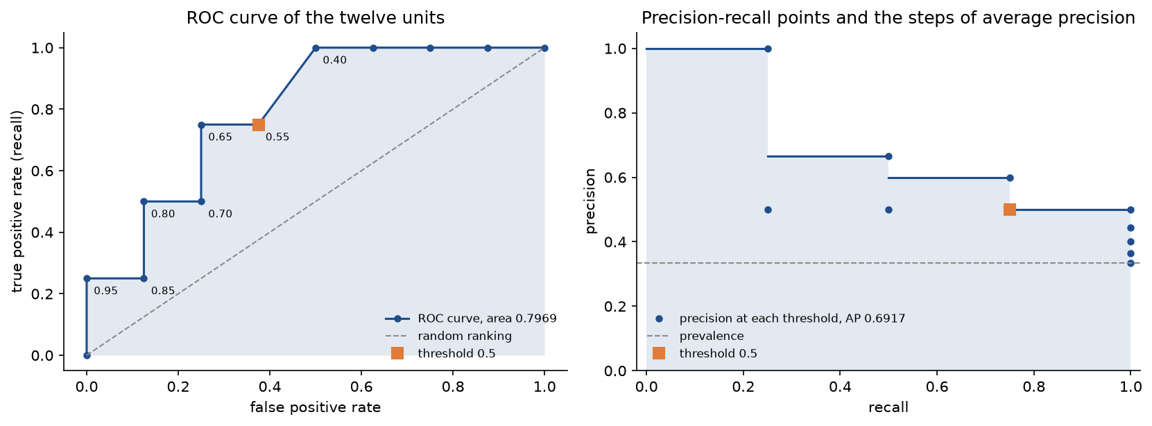
On the left, the diagonal segment from (0.375, 0.75) to (0.5, 1) is the tied pair entering together. On the right, the four blue steps sit at the precisions reached where recall rises; the points below them are the sawtooth that average precision ignores.

A threshold chosen by cost

A missed faulty unit costs 10 and a false alarm costs 1. The total cost FP + 10 FN at each threshold of the list, from the infinite threshold down to 0.10, is 40, 30, 31, 21, 22, 12, 13, 4, 5, 6, 7 and 8. The cheapest threshold is 0.40, flagging units 1 to 8 for a cost of 4 (four false alarms, no misses). The default 0.5 costs 13, more than three times as much, because it misses unit 8. In ROC terms, the iso-cost slope is 1 · (8/12) / (10 · 4/12) = 0.2, a shallow line that touches the curve at its highest corner (0.5, 1). If the scores were calibrated probabilities the threshold would be 1/(1 + 10) = 0.0909, which flags all twelve units for a cost of 8. The empirical minimum and the formula disagree because these scores are not calibrated, as the next section shows, and twelve units are far too few to choose a threshold from anyway.

Calibration

The squared errors of the faulty units are 0.05², 0.20², 0.35² and 0.60², summing to 0.525, and those of the working units are 0.85², 0.70², 0.55², 0.40², 0.30², 0.20², 0.15² and 0.10², summing to 1.8375. The Brier score is (0.525 + 1.8375) / 12 = 2.3625 / 12 = 0.196875, shown as 0.1969. Forecasting the base rate 1/3 for every unit scores (1/3)(2/3) = 0.2222, so the model beats the base-rate forecast, but only by 0.0253.

With two bins, from 0 to 0.5 and from just above 0.5 to 1, the reliability diagram has two points:

• The lower bin holds units 7 to 12, with mean score 1.55 / 6 = 0.2583 and observed share faulty 1/6 = 0.1667, a gap of 0.0917.
• The upper bin holds units 1 to 6, with mean score 4.5 / 6 = 0.75 and observed share faulty 3/6 = 0.5, a gap of 0.25.

The expected calibration error is (6/12) · 0.0917 + (6/12) · 0.25 = 0.1708. In the upper bin the model says 75 % and is right half the time: it is overconfident, and a threshold computed from these scores as if they were probabilities will be wrong.

How sure are we?

Accuracy at threshold 0.5 is 8 correct out of 12. With z = 1.959964, the 97.5 % point of the standard normal distribution usually rounded to 1.96, z² is 3.8415:

• Wald: 0.6667 ± 1.96 √(0.6667 · 0.3333 / 12) = 0.6667 ± 0.2667, the interval from 0.3999 to 0.9334.
• Wilson: the centre is (0.6667 + 3.8415/24) / (1 + 3.8415/12) = 0.8267 / 1.3201 = 0.6263 and the half-width is 1.96 √(0.018519 + 3.8415/576) / 1.3201 = 1.96 · 0.1587 / 1.3201 = 0.2356, giving 0.3906 to 0.8619.
• Percentile bootstrap, 2,000 resamples of the twelve units: 0.4167 to 0.9167.

All three say the same thing: twelve units cannot tell an accuracy of 0.4 from one of 0.9. The bootstrap interval for the AUC runs from 0.4831 to 1.0000 and includes a model no better than chance; 17 of the 2,000 resamples contained no faulty unit and were skipped, close to the expected 2000 · (8/12)¹² = 15.4.

Three classes

Seventy parts are graded good, rework or scrap. Of the 50 good parts the grader calls 46 good, 3 rework and 1 scrap; of the 15 rework parts, 5 good, 9 rework and 1 scrap; of the 5 scrap parts, 1 good, 2 rework and 2 scrap. The column totals, the parts predicted in each grade, are 52, 14 and 4.

• Good: precision 46/52 = 0.8846, recall 46/50 = 0.9200, F1 92/102 = 0.9020, support 50.
• Rework: precision 9/14 = 0.6429, recall 9/15 = 0.6000, F1 18/29 = 0.6207, support 15.
• Scrap: precision 2/4 = 0.5000, recall 2/5 = 0.4000, F1 4/9 = 0.4444, support 5.
• Macro averages: precision 0.6758, recall 0.6400, F1 (0.9020 + 0.6207 + 0.4444)/3 = 0.6557.
• Weighted averages: precision 0.8053, recall 0.8143, F1 (50 · 0.9020 + 15 · 0.6207 + 5 · 0.4444)/70 = 0.8090.
• Micro averages: precision, recall and F1 all equal the accuracy, 57/70 = 0.8143, as does the weighted recall.

The other macro F1, the harmonic mean of the macro precision 0.6758 and the macro recall 0.6400, is 0.6574.

For the chance-corrected measures, the row totals are 50, 15 and 5 and the column totals 52, 14 and 4, so the sum of their products is 2600 + 210 + 20 = 2830. The expected agreement is 2830 / 4900 = 0.5776 and kappa is (0.8143 - 0.5776) / (1 - 0.5776) = 0.5604. The MCC is (57 · 70 - 2830) / √((4900 - 2916)(4900 - 2750)) = 1160 / 2065.33 = 0.5617. The grades are ordered, and most errors are between neighbouring grades, so the quadratically weighted kappa is higher, 0.6145.

A grader that calls every part good has accuracy 50/70 = 0.7143, weighted F1 0.5952 (the good class's F1, 0.8333, times 50/70) and macro F1 0.2778, while its MCC and kappa are exactly 0. Its weighted F1 is more than twice its macro F1; only the chance-corrected measures say plainly that it has learned nothing.

Regression

Six households use 12, 20, 15, 30, 8 and 25 kWh a day, and a model forecasts 14, 18, 15, 24, 11 and 27. The errors are 2, -2, 0, -6, 3 and 2, and the absolute percentage errors 0.1667, 0.1000, 0, 0.2000, 0.3750 and 0.0800.

• MSE = (4 + 4 + 0 + 36 + 9 + 4) / 6 = 57/6 = 9.5 and RMSE = √9.5 = 3.0822.
• MAE = 15/6 = 2.5.
• MAPE = 0.9217 / 6 = 0.1536.
• The mean of the actual values is 110/6 = 18.3333, the total sum of squares 341.3333, and R² = 1 - 57/341.3333 = 0.8330.

Household 5 has an absolute error of only 3 kWh, yet it contributes 0.375 of the 0.9217 percentage-error sum because its target is the smallest.

Which constant forecast does each metric prefer? MSE is smallest at the mean, 18.3333 (MSE 56.8889). MAE is smallest anywhere between the two middle values, 15 and 20 (MAE 6.6667). MAPE is smallest at the median weighted by 1/y: sorted, the targets 8, 12, 15, 20, 25 and 30 have weights 0.125, 0.0833, 0.0667, 0.05, 0.04 and 0.0333 summing to 0.3983, and the cumulative weight first reaches half of that, 0.1992, at 12. The constant 12 has MAPE 0.3700 against 0.4424 at the median 17.5, and MAE 7.6667 against 6.6667: optimizing MAPE pulls forecasts well below the typical value.

Cross-validation folds

Four folds of the twelve units in the order of the list. Plain 4-fold takes consecutive blocks, units 1 to 3, 4 to 6, 7 to 9 and 10 to 12, which contain 2, 1, 1 and 0 faulty units; the last fold's recall is undefined. Stratified 4-fold deals the classes round-robin: each fold gets one of the four faulty units and two of the eight working ones, in order of appearance. At threshold 0.5:

• Fold of units 1, 2 and 4: TP 1, FP 2, FN 0; precision 0.3333, recall 1, F1 0.5000.
• Fold of units 3, 6 and 7: TP 1, FP 1, FN 0; precision 0.5000, recall 1, F1 0.6667.
• Fold of units 5, 9 and 10: TP 1, FP 0, FN 0; precision 1, recall 1, F1 1.
• Fold of units 8, 11 and 12: TP 0, FP 0, FN 1; precision undefined and counted as 0, recall 0, F1 0.

The mean over the folds is precision 0.4583, recall 0.75 and F1 0.5417, while the pooled values over all twelve units are precision 0.5000, recall 0.75 and F1 0.6000. The fold average understates both precision and F1, partly because the last fold flags nothing and its precision of 0/0 is counted as 0. Recall agrees with the pooled value here, and not by accident: when every fold holds the same number of positives, the mean of the fold recalls is the total number of true positives over P, the pooled recall.

Every number in this section is asserted by the tests of the module it belongs to, for example tests/test_rates.py for the rates and tests/test_curves.py for the curves, and printed by examples/worked_example.py, examples/classes_and_regression.py and examples/folds_and_intervals.py.

The code

The package evaluation_metrics is plain NumPy and the standard library, split into one module per idea. scikit-learn and SciPy are imported only inside the functions of comparisons.py and the data loader breast_cancer, so everything else works without them.

• arrays.py holds the array types, the input checks and ratio, which returns 0 or another chosen value for a zero denominator.
• counts.py holds confusion_matrix (rows actual, columns predicted), the frozen BinaryCounts with binary_counts, counts_at_threshold, one_vs_rest and counts_from_matrix.
• rates.py holds accuracy, precision, recall, specificity, the false positive rate, the negative predictive value, f_beta, f1, balanced accuracy, and matthews_correlation and cohen_kappa, which accept two-class counts or a K by K matrix.
• averaging.py holds per_class_scores, averaged_scores for macro, micro and weighted averages, and f1_of_macro_averages, the other macro F1.
• curves.py holds threshold_table, the core of every curve, roc_curve, roc_auc, precision_recall_curve, average_precision and two operating points, precision_at_recall and recall_at_false_positive_rate.
• ranking.py holds the AUC as a probability: pairwise_auc by explicit pairs and rank_auc by the Mann-Whitney rank sum.
• costs.py holds cost_curve, best_threshold, bayes_threshold and iso_cost_slope.
• calibration.py holds brier_score, brier_decomposition, reliability_curve and expected_calibration_error with uniform or quantile bins, PlattScaling, and PlattCalibrated, which fits Platt scaling on inner cross-validated scores.
• models.py holds the two classifiers the project evaluates: LogisticRegression (Newton's method on standardized features with an L2 penalty) and GaussianNaiveBayes, both frozen dataclasses with fit, predict_proba and decision_function.
• regression.py holds MSE, RMSE, MAE, MAPE, R² and mape_optimal_constant.
• cross_validation.py holds k_fold, stratified_k_fold, group_k_fold and time_series_split, each returning the same indices as scikit-learn's splitter, and out_of_fold_probabilities.
• intervals.py holds wald_interval, wilson_interval, bootstrap_interval over rows or whole groups, and bootstrap_difference for paired comparisons.
• worked_example.py builds the data of the section above; datasets.py generates binormal scores, Gaussian classes and clustered answers, and loads the breast-cancer data.
• studies.py, forecast_study.py and pitfalls.py hold the simulation studies and demonstrations quoted under In practice and Pitfalls.
• reports.py prints confusion matrices, threshold tables and classification reports; plotting.py and diagnostics.py draw every figure in the handbook's four colours.
• comparisons.py computes the largest differences from scikit-learn and SciPy.

Every curve starts from threshold_table, which sorts the scores once, accumulates the counts and keeps the last row of each run of equal scores, so a group of tied examples enters as one step:

order = np.argsort(-scores, kind="stable")
sorted_scores = scores[order]
sorted_positive = is_positive[order]
true_positives = np.cumsum(sorted_positive)
false_positives = np.cumsum(~sorted_positive)
last_of_each_score = np.r_[sorted_scores[1:] != sorted_scores[:-1], True]

From the table, roc_curve prepends the point (0, 0) for the infinite threshold, precision_recall_curve returns precision and recall at the same thresholds, and average precision is one line, np.sum(np.diff(np.r_[0.0, table.recall]) * table.precision). Functions that take scores return nan when a metric is undefined, for example the AUC of data with one class only, so that bootstrap_interval can skip such resamples and report how many it skipped.

The examples and the project import the package, so install the repository first as described in the main README. Each example demonstrates one idea and runs in a few seconds at most from the repository root:

• examples/worked_example.py prints every number of the two-class worked example in the order above and draws its ROC and precision-recall figure.
• examples/classes_and_regression.py prints the three-class grades, the grader that calls everything good, the three-class run that never predicts its rare class, and the household forecasts with the best constant for each error measure.
• examples/imbalance_study.py runs the prevalence study and the two-model comparison of In practice and draws both figures.
• examples/folds_and_intervals.py prints the folds of the twelve units, draws the four splitters on 24 rows, counts folds without a positive over 200 shuffles, compares the Wald and Wilson intervals, resamples answers and people, and checks the coverage of the percentile bootstrap; it is the slowest example at a few seconds.
• examples/common_mistakes.py demonstrates the AUC of hard predictions, the trapezoid rule in precision-recall space, tie handling, a swapped positive class, the two macro F1 scores and the regression pitfalls on a demand forecast.
• examples/compare_with_sklearn.py prints the largest difference between each function and scikit-learn or SciPy.

python machine-learning/evaluation-metrics/examples/worked_example.py
python machine-learning/evaluation-metrics/examples/classes_and_regression.py
python machine-learning/evaluation-metrics/examples/imbalance_study.py
python machine-learning/evaluation-metrics/examples/folds_and_intervals.py
python machine-learning/evaluation-metrics/examples/common_mistakes.py
python machine-learning/evaluation-metrics/examples/compare_with_sklearn.py

The sample project, project/evaluation_report.py, writes a complete evaluation report for a screening task on the breast-cancer data: two classifiers, logistic regression and Gaussian naive Bayes, and a copy of naive Bayes recalibrated by Platt scaling.

The order matters more than any single metric. The test set is locked away first; every choice, the threshold included, is made on out-of-fold probabilities of the development set; the test set is scored once. The report prints the out-of-fold metrics of each model, the threshold chosen on the development set and the Bayes threshold with their test costs, and the test AUC, average precision and Brier score with 95 % bootstrap intervals and paired differences, and saves three figures. Options such as --seed, --folds, --penalty, --false-positive-cost, --false-negative-cost and --resamples change the setup, and --figures sends the PNGs to another folder so a custom run does not overwrite the ones shown here. The default run takes about two seconds; its results are discussed under In practice.

python machine-learning/evaluation-metrics/project/evaluation_report.py
python machine-learning/evaluation-metrics/project/evaluation_report.py --false-negative-cost 50 --seed 3

The notebook evaluation_metrics.ipynb is a guided tour in the order of this page: the worked example, multiclass averaging, regression metrics and cross-validation folds, a demonstration of each pitfall, the imbalance study, the screening run and the comparison with scikit-learn. The tests in tests check the worked example value by value, the mathematical properties above and the agreement with scikit-learn, and run in a few seconds:

python -m pytest machine-learning/evaluation-metrics

Data: the worked example, the imbalance study, the three-class run, the demand series and the pitfall demonstrations use small fixed numbers or synthetic data generated from fixed seeds by the package. The screening project uses the Breast Cancer Wisconsin (Diagnostic) data set by W. Wolberg, W. Street and O. Mangasarian from the UCI Machine Learning Repository, licensed CC BY 4.0, which ships with scikit-learn, so nothing is downloaded.

In practice

The same in scikit-learn

Every function has a scikit-learn counterpart, and the counterparts differ only in conventions:

• confusion_matrix matches metrics.confusion_matrix, with the same layout, rows actual.
• per_class_scores and averaged_scores match metrics.precision_recall_fscore_support with average=None, "macro", "micro" or "weighted".
• f_beta, matthews_correlation and cohen_kappa match fbeta_score, matthews_corrcoef and cohen_kappa_score, which takes weights="linear" or "quadratic".
• roc_curve matches metrics.roc_curve with drop_intermediate=False; the default drops collinear points, which changes the arrays but not the area. roc_auc matches roc_auc_score.
• precision_recall_curve matches metrics.precision_recall_curve reversed: scikit-learn orders by increasing threshold and appends the point at recall 0 and precision 1. average_precision matches average_precision_score, a step sum, not trapezoids.
• brier_score matches brier_score_loss, and reliability_curve matches calibration.calibration_curve, with the same right-closed bins and empty bins dropped.
• PlattCalibrated corresponds to calibration.CalibratedClassifierCV(method="sigmoid"), which also smooths the targets and by default averages one calibrated copy per fold.
• The regression functions match mean_squared_error, root_mean_squared_error, mean_absolute_error, mean_absolute_percentage_error and r2_score; r2_score returns 1 or 0 instead of nan for constant targets.
• The splitters match KFold, StratifiedKFold, GroupKFold and TimeSeriesSplit index for index, including shuffling with the same seed.
• wilson_interval matches scipy.stats.binomtest(...).proportion_ci(method="wilson").

In examples/compare_with_sklearn.py, every metric, curve, calibration curve and regression metric agrees with scikit-learn exactly or to within 1.1 × 10⁻¹⁶, every splitter index for index, the logistic regression's probabilities to 1.4 × 10⁻¹¹ (against newton-cholesky with a tolerance of 10⁻¹²), Gaussian naive Bayes to 1.7 × 10⁻¹⁵ and the Wilson interval to 5.6 × 10⁻¹⁷. The tests repeat these comparisons on other data. Use scikit-learn in practice: it handles sample weights, multilabel targets and the edge cases. The package exists to make each formula visible and checkable.

Imbalance: what moves and what does not

The imbalance study draws binormal scores, negatives from the standard normal distribution and positives from a normal distribution with mean 2 and standard deviation 1, with 20,000 negatives and enough positives for prevalences of 50 %, 10 % and 1 %. The theoretical AUC is Φ(√2) = 0.9214 at every prevalence. A model flags the scores of at least 1, and a silent classifier never flags anything.

• 50 % positives (20,000): AUC 0.9217, AP 0.9224. The model has accuracy 0.8422, balanced accuracy 0.8422, precision 0.8416, recall 0.8431, F1 0.8424, MCC 0.6845 and kappa 0.6845. The silent classifier has accuracy 0.5000.
• 10 % positives (2,222): AUC 0.9255, AP 0.6819. The model has accuracy 0.8416, balanced accuracy 0.8452, precision 0.3722, recall 0.8497, F1 0.5176, MCC 0.4935 and kappa 0.4397. The silent classifier has accuracy 0.9000.
• 1 % positives (202): AUC 0.9238, AP 0.3020. The model has accuracy 0.8404, balanced accuracy 0.8581, precision 0.0524, recall 0.8762, F1 0.0989, MCC 0.1910 and kappa 0.0816. The silent classifier has accuracy 0.9900.

The ROC area, recall and balanced accuracy stay where they are, because they condition on the true class. Average precision falls from 0.92 to 0.30 and precision from 0.84 to 0.05, close to the 0.0508 the precision formula predicts. Accuracy hardly moves for the model and climbs to 0.99 for the classifier that does nothing, which beats the model at 10 % and 1 % prevalence; the MCC and kappa of the silent classifier stay at 0 throughout.

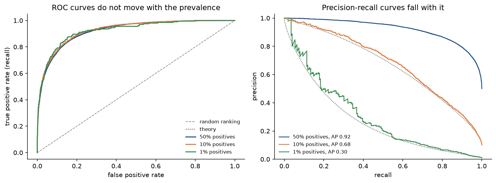
The left panel cannot tell the three data sets apart; the right panel can tell nothing else. The dotted curves are the exact binormal curves, computed from the precision formula, and the noisy 1 % curve shows how few positives decide the top of the ranking.

The second experiment compares two scoring models at 1 % prevalence, 200 positives among 20,000. Model A has positives from a normal distribution with mean 2 and standard deviation 1, model B with mean 2.6 and standard deviation 2, a wider spread that puts some positives far above every negative and others among them. In theory B has the lower AUC, Φ(2.6/√5) = 0.8775 against 0.9214.

• Model A: AUC 0.9239, AP 0.3093, recall 0.4000 at a 1 % false positive rate, precision 0.1969 at 50 % recall.
• Model B: AUC 0.8942, AP 0.4940, recall 0.5250 at a 1 % false positive rate, precision 0.3788 at 50 % recall.

The AUC prefers A by 0.03. Everywhere an application with 1 % positives could operate, B is better: at a 1 % false alarm rate it catches 52.5 % of the positives instead of 40 %, and at 50 % recall nearly two of every five alarms are real instead of one in five. B's advantage lives at false positive rates below a few percent, a sliver of the ROC plot's width that the AUC averages away; the precision-recall curve is drawn in exactly that region.

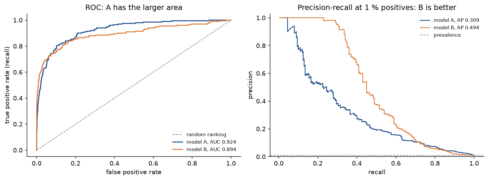
The two panels rank the models in opposite orders. Only the right one shows the region an application with rare positives works in.

A realistic run: screening for malignant tumours

The breast-cancer data hold 569 tumours with 30 features each; malignant is the positive class, 212 cases (37.3 %). The project locks away the first fold of a shuffled stratified four-fold split as the test set, 143 tumours of which 53 are malignant. On the remaining 426, the development set, stratified five-fold cross-validation produces out-of-fold probabilities for three models: logistic regression with penalty 1, Gaussian naive Bayes, and naive Bayes recalibrated by Platt scaling on inner three-fold scores. At threshold 0.5:

• Logistic regression: accuracy 0.9812, precision 0.9809, recall 0.9686, F1 0.9747, MCC 0.9598; AUC 0.9976, AP 0.9964, Brier score 0.0159, ECE 0.0120.
• Naive Bayes: accuracy 0.9413, precision 0.9408, recall 0.8994, F1 0.9196, MCC 0.8740; AUC 0.9886, AP 0.9779, Brier score 0.0534, ECE 0.0549.
• Naive Bayes with Platt scaling: accuracy 0.9390, precision 0.9524, recall 0.8805, F1 0.9150, MCC 0.8692; AUC 0.9902, AP 0.9846, Brier score 0.0406, ECE 0.0431.

Naive Bayes multiplies thirty strongly correlated likelihoods as if they were independent, which pushes almost every probability to 0 or 1; the reliability diagrams show it. Platt scaling leaves each fold's ranking unchanged, but it lowers the Brier score from 0.0534 to 0.0406. Its pooled AUC differs slightly from naive Bayes' because each fold has its own Platt map, so pooling mixes five slightly different scales.

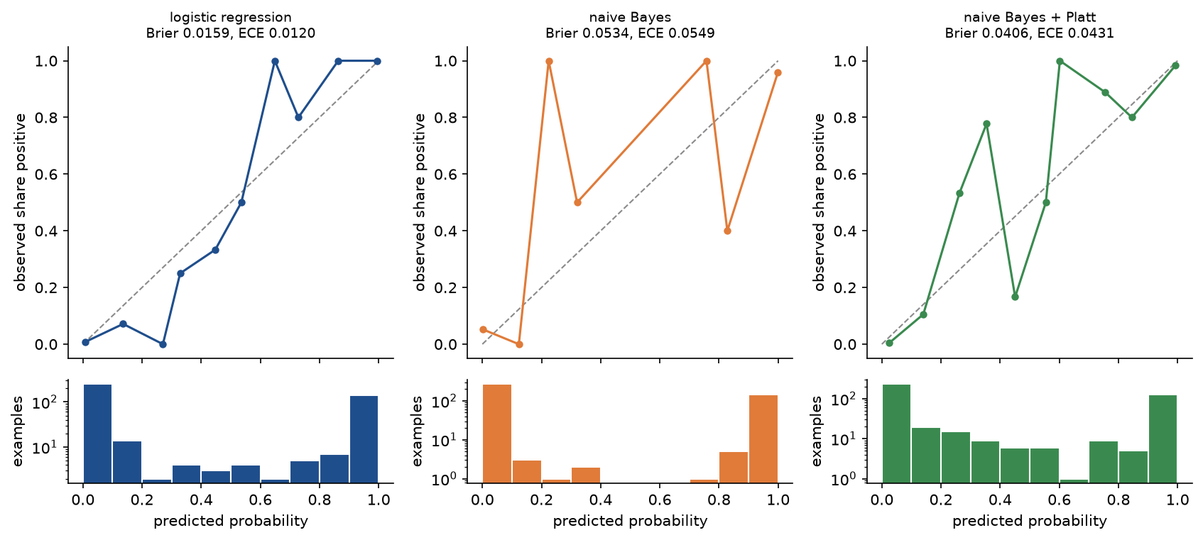
The histograms carry the story. Naive Bayes has almost nothing between 0.1 and 0.9, so its few middle bins hold a handful of tumours each and swing wildly; after Platt scaling the predictions spread out and the diagram moves towards the diagonal.

Now suppose a missed malignant tumour costs 20 times as much as a false alarm, so the Bayes threshold is 1/21 = 0.0476. The threshold is chosen to minimize the total cost on the development set's out-of-fold probabilities; then every model is refitted on the whole development set and scored once on the test set at three thresholds:

• Logistic regression: the default 0.5 costs 82 (4 missed, 2 false alarms); the threshold 0.05209 chosen on the development set costs 34 (1 missed, 14 false alarms); the Bayes threshold also costs 34 (1 missed, 14 false alarms).
• Naive Bayes: the default costs 143 (7 missed, 3 false alarms); the chosen threshold, 1.836 × 10⁻⁷, costs 54 (2 missed, 14 false alarms); the Bayes threshold costs 144 (7 missed, 4 false alarms).
• Naive Bayes with Platt scaling: the default costs 143 (7 missed, 3 false alarms); the chosen threshold 0.1041 costs 53 (2 missed, 13 false alarms); the Bayes threshold costs 40 (1 missed, 20 false alarms).

Three lessons in one list. For every model the default threshold costs 2.4 to 3.6 times as much on the test set as the cheaper of the other two. For the calibrated logistic regression the threshold searched on development data (0.05209) and the one computed from the costs (0.0476) agree and give the same test cost, less than half that of the default. For naive Bayes the computed threshold is useless, cost 144, because its "probabilities" are not probabilities, and the searched threshold, 1.836 × 10⁻⁷, shows how far they are from the truth; after Platt scaling the computed threshold works again (cost 40).

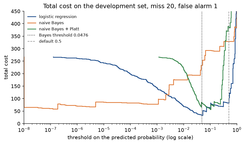
Each curve is a staircase in the threshold, and the cheapest step is where its minimum sits. Only the calibrated model has its minimum at the threshold the costs predict; the uncalibrated one has its minimum at 1.836 × 10⁻⁷, more than five orders of magnitude below it.

On the test set, with 95 % percentile intervals from 2,000 bootstrap resamples:

• Logistic regression: AUC 0.9874 (0.9677 to 0.9991), AP 0.9849 (0.9618 to 0.9986), Brier score 0.0320 (0.0126 to 0.0577).
• Naive Bayes: AUC 0.9816 (0.9613 to 0.9950), AP 0.9733 (0.9441 to 0.9923), Brier score 0.0708 (0.0337 to 0.1144).
• Naive Bayes with Platt scaling: AUC 0.9816, the same ranking, and Brier score 0.0555.

The two AUC intervals overlap almost completely, and the paired bootstrap of the difference, logistic minus naive Bayes, gives +0.0059 with interval -0.0072 to +0.0202: on 143 tumours the two models cannot be told apart by their ranking. The paired difference in Brier score, -0.0388 with interval -0.0743 to -0.0051, excludes zero: the logistic regression's probabilities are reliably better, which is the property the threshold choice depended on.

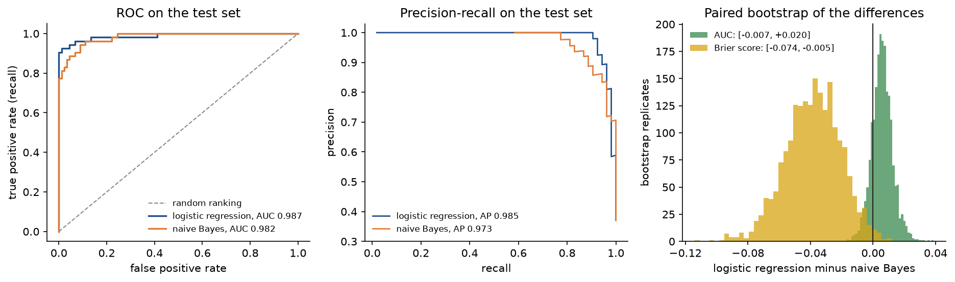
The right panel is the whole argument of the paired bootstrap: one distribution straddles zero and one does not, although the separate intervals of both quantities overlap.

Does the percentile interval deserve its name?

On 200 simulated test sets of 200 binormal scores (60 positives, separation 1.5, true AUC Φ(1.5/√2) = 0.8556), the 95 % intervals from 500 resamples each covered the true AUC 187 times, 93.5 %, with a mean width of 0.1117. With 200 repetitions the coverage estimate itself has a standard error of about 1.5 points, so this is consistent with 95 %. examples/folds_and_intervals.py runs the check.

Three classes

Gaussian naive Bayes on three synthetic classes of 1,500, 400 and 100 examples, evaluated by stratified five-fold cross-validation, and then the same model forbidden to predict the rare class:

• All three classes: accuracy 0.8725, macro F1 0.7211, weighted F1 0.8667, balanced accuracy 0.6822, MCC 0.6613, kappa 0.6586, rare-class recall 0.4100.
• Never predicts the rare class: accuracy 0.8580, macro F1 0.5392, weighted F1 0.8363, balanced accuracy 0.5543, MCC 0.6187, kappa 0.6132, rare-class recall 0.

Abandoning a class entirely costs 0.03 of weighted F1 and 0.015 of accuracy, but 0.18 of macro F1 and 0.13 of balanced accuracy. Report macro averages, or the per-class scores, whenever the small classes matter.

Choosing what to report

• Balanced classes and errors of similar cost: accuracy with an interval, and the confusion matrix.
• Rare positives, and the positives are what matters: precision, recall and F1 at the operating threshold, average precision and the precision-recall curve, and the prevalence as the baseline.
• Comparing rankings across data sets with different balance: ROC AUC, ideally with the ROC curve.
• A single balanced summary of hard predictions: the MCC, or balanced accuracy.
• Agreement with a reference rater: Cohen's kappa, quadratically weighted for ordered classes.
• Several classes: the per-class scores, macro averages for small classes, and which macro F1.
• Decisions with known costs: the expected cost at the chosen threshold, from calibrated probabilities and the Bayes threshold or from a threshold chosen on validation data.
• Probabilities used downstream: the Brier score or log loss, and a reliability diagram.
• Regression: MAE and RMSE in target units; avoid MAPE near zero targets; R² only alongside an absolute error.
• Any of the above: how the scores were produced (splitter and folds), a confidence interval, and a baseline.

When to use which implementation:

• Use the from-scratch package to learn what each number means, to compute a metric by hand and check it, and to read papers that define their own variants.
• Use scikit-learn for real work. It is faster, handles sample weights, multilabel and multiclass inputs and the edge cases, and is what reviewers expect.
• Use the bootstrap functions of either, or scipy.stats.bootstrap, whenever a number is reported; the BCa variant there improves the percentile interval for skewed metrics.

Pitfalls

• Computing ROC AUC from hard predictions. Passing 0 or 1 labels to roc_auc_score returns a number, but it is the balanced accuracy, not an area under a ranking. On the worked example the scores give 0.7969 and the predictions at 0.5 give 0.6875, exactly the balanced accuracy (examples/common_mistakes.py). Pass predict_proba or decision_function output.
• Trapezoidal area under a precision-recall curve. auc(recall, precision) interpolates linearly between operating points, which no classifier can achieve, and does not equal average precision. On fine curves it lands slightly low (0.3830 against an AP of 0.3942 for 20 positives among 2,000 scores); on hard predictions with scikit-learn's starting point at precision 1 it gives 0.4888 where AP gives 0.1952 (tests/test_pitfalls.py). Use average_precision_score.
• Ignoring ties. Stepping through the sorted list one row at a time instead of one distinct score at a time makes the curve depend on how the sort orders tied rows. In the worked example the tied units 7 and 8 give an area of 25/32 = 0.78125 in one order and 26/32 = 0.8125 in the other; grouping them gives 0.796875, the pairwise probability with ties counted one half. Ties are common with rounded scores, trees and small ensembles.
• Accuracy under imbalance. At 1 % prevalence a classifier that never flags anything has accuracy 0.99 and beats a model with recall 0.88 (accuracy 0.8404). Report the prevalence, a majority-class baseline and class-conditional measures. The opposite error is just as common: declaring one metric "the right one for fraud" or "for medicine". Precision matters when false alarms are expensive, recall when misses are, and the costs, not the domain, decide.
• Weighted averages hide small classes. A model that never predicts the rare class loses 0.03 of weighted F1 and 0.18 of macro F1 in the three-class run. Weighted recall and micro F1 are identical to accuracy for single-label problems (tests/test_averaging.py), so reporting them next to accuracy adds nothing.
• Two macro F1 scores. The mean of the per-class F1 scores (0.6557 on the graded parts, scikit-learn's definition) and the F1 of the macro precision and recall (0.6574) differ, sometimes by much more. Say which one a report contains.
• Choosing the positive class silently. Precision, recall and F1 describe one class. Calling the working units positive instead of the faulty ones turns precision 0.5, recall 0.75 and F1 0.6 into 0.8333, 0.625 and 0.7143, while accuracy, MCC and kappa do not move. Set pos_label explicitly, especially with string labels, where scikit-learn either refuses to guess or, for the ranking metrics, takes the label that sorts last as positive.
• Reading a transposed confusion matrix. Some texts put predictions in the rows or the positive class first; reading precision off the wrong axis gives the recall. Label both axes, and remember that ravel() on scikit-learn's binary matrix returns TN, FP, FN, TP.
• Threshold 0.5 by default, or a threshold tuned on the test set. The default threshold cost 82 against 34 for the cost-based threshold in the screening run. The threshold is a model parameter: choose it on validation or out-of-fold data, then report the test score at that threshold. A threshold chosen on the test set makes the test score optimistic, the selection bias that Data leakage and pitfalls quantifies.
• Computing a threshold from uncalibrated probabilities. The Bayes threshold assumes calibrated probabilities. Applied to naive Bayes it cost 144 on the test set against 40 after Platt scaling. A high AUC says nothing about calibration: Platt scaling left naive Bayes' test AUC at exactly 0.9816 while its Brier score fell from 0.0708 to 0.0555.
• Calibrating on the training data. Platt scaling or isotonic regression fitted on the scores of the data the model was trained on learns the model's overconfidence on that data. Fit the calibrator on held-out or inner cross-validated scores, as PlattCalibrated and CalibratedClassifierCV do.
• Averaging fold metrics instead of pooling, or pooling without thinking. On the worked example's stratified folds the mean F1 is 0.5417 and the pooled F1 0.6000; the mean of five forward-chaining fold RMSEs on a demand series is 1.7266 against a pooled 1.7527, and the mean of the square roots is always the smaller. Pooling is not automatically right either: it treats scores from different fold models as one scale, which moved the pooled AUC of the Platt-scaled model from 0.9886 to 0.9902. Say which you did, and keep fold sizes equal.
• Folds without positives. With 10 positives among 200 rows, shuffled ten-fold cross-validation produced 665 folds without a positive in 2,000 (the expected number is 2000 · 0.3398 = 679.5), each with an undefined recall; stratified folds produced none (examples/folds_and_intervals.py). Use StratifiedKFold for classification, and StratifiedGroupKFold when groups must be kept together as well.
• MAPE with zero or small targets. On a synthetic demand series of two years, with 96 days without a sale, the MAPE of a linear forecast on the last 182 days is 8.7 × 10¹⁴; on the days with a sale it is 0.7523 (examples/common_mistakes.py). Even without zeros, MAPE punishes over-forecasts more than under-forecasts, and the best constant under MAPE for the six households is 12 kWh against a median of 17.5. Prefer MAE or RMSE, or a scaled error such as MASE, which divides by the error of a naive forecast.
• Misreading R². A negative R² on test data is not a bug: the training mean used as a forecast for the test period of the demand series scores -0.3720, because R² measures against the test period's own mean. A common slip writes the denominator as the spread of the predictions; the reference is the spread of the actual values. And R² equals the squared correlation only for a least-squares fit with an intercept on its own training data (tests/test_regression.py).
• Resampling the wrong unit. Thirty people answering twenty questions each are thirty independent units, not 600. Resampling answers gives an accuracy interval from 0.6133 to 0.6883 with standard deviation 0.0192; resampling people gives 0.5783 to 0.7217 with 0.0355; the real spread over 2,000 fresh groups of people is 0.0420 (examples/folds_and_intervals.py). Bootstrap, and cross-validate, over the unit that is independent.

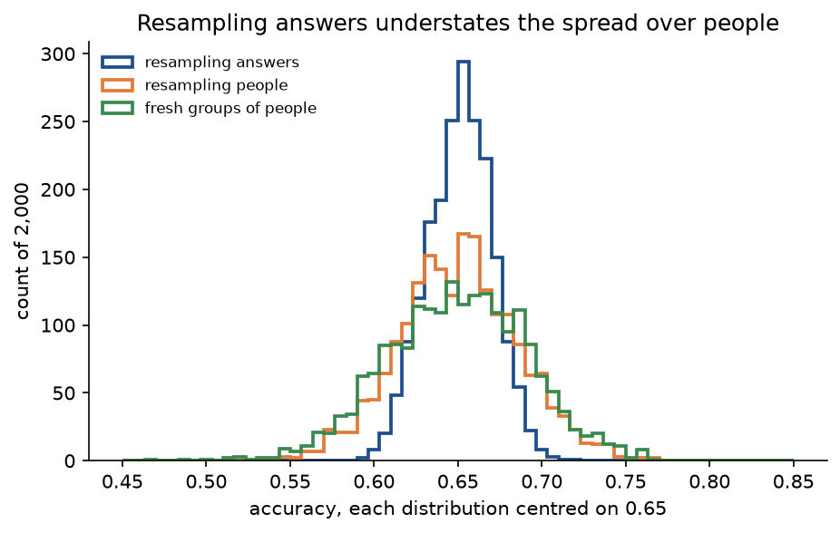
The narrow blue peak is the confidence the wrong bootstrap claims; the orange and green distributions, which agree with each other, are the uncertainty that is really there.

• Comparing models with separate intervals. Two overlapping intervals do not mean two models are indistinguishable, and two separate ones overstate the uncertainty of the difference, because both models err on the same hard cases. Use a paired bootstrap of the difference, as for the Brier scores of the screening run, whose separate intervals overlap but whose paired difference excludes zero.
• Too few examples for the metric. Twelve units give an accuracy interval from 0.39 to 0.86 and an AUC interval that includes 0.5. A metric is only as precise as the number of examples in its denominator: recall on 53 malignant tumours is a proportion of 53, not of 143.

Further reading

• T. Fawcett, "An introduction to ROC analysis", Pattern Recognition Letters 27(8), 861-874, 2006. ROC space, the AUC and its probabilistic meaning, iso-cost lines.
• J. A. Hanley and B. J. McNeil, "The meaning and use of the area under a receiver operating characteristic (ROC) curve", Radiology 143(1), 29-36, 1982. The AUC as the Mann-Whitney statistic and its standard error.
• J. Davis and M. Goadrich, "The relationship between precision-recall and ROC curves", Proceedings of the 23rd International Conference on Machine Learning, 2006. Why linear interpolation in precision-recall space is wrong.
• T. Saito and M. Rehmsmeier, "The precision-recall plot is more informative than the ROC plot when evaluating binary classifiers on imbalanced datasets", PLOS ONE 10(3), e0118432, 2015.
• B. W. Matthews, "Comparison of the predicted and observed secondary structure of T4 phage lysozyme", Biochimica et Biophysica Acta 405(2), 442-451, 1975. The origin of the Matthews correlation coefficient.
• J. Gorodkin, "Comparing two K-category assignments by a K-category correlation coefficient", Computational Biology and Chemistry 28(5-6), 367-374, 2004. The multiclass MCC.
• D. Chicco and G. Jurman, "The advantages of the Matthews correlation coefficient (MCC) over F1 score and accuracy in binary classification evaluation", BMC Genomics 21, 6, 2020.
• J. Cohen, "A coefficient of agreement for nominal scales", Educational and Psychological Measurement 20(1), 37-46, 1960, and "Weighted kappa", Psychological Bulletin 70(4), 213-220, 1968.
• C. J. van Rijsbergen, Information Retrieval, second edition, Butterworths, 1979, chapter 7. The effectiveness measure behind F-beta.
• J. Opitz and S. Burst, "Macro F1 and Macro F1", arXiv:1911.03347, 2019. The two macro F1 definitions and how far apart they can be.
• G. W. Brier, "Verification of forecasts expressed in terms of probability", Monthly Weather Review 78(1), 1-3, 1950, and A. H. Murphy, "A new vector partition of the probability score", Journal of Applied Meteorology 12(4), 595-600, 1973.
• J. C. Platt, "Probabilistic outputs for support vector machines and comparisons to regularized likelihood methods", in Advances in Large Margin Classifiers, MIT Press, 1999.
• A. Niculescu-Mizil and R. Caruana, "Predicting good probabilities with supervised learning", Proceedings of the 22nd International Conference on Machine Learning, 2005. Which models are calibrated out of the box, and Platt versus isotonic recalibration.
• C. Elkan, "The foundations of cost-sensitive learning", Proceedings of the 17th International Joint Conference on Artificial Intelligence, 2001. The cost-optimal threshold and its dependence on the class prior.
• R. J. Hyndman and A. B. Koehler, "Another look at measures of forecast accuracy", International Journal of Forecasting 22(4), 679-688, 2006. The problems of MAPE and the scaled alternative MASE.
• G. Forman and M. Scholz, "Apples-to-apples in cross-validation studies: pitfalls in classifier performance measurement", ACM SIGKDD Explorations 12(1), 49-57, 2010. Averaging versus pooling over folds.
• R. Kohavi, "A study of cross-validation and bootstrap for accuracy estimation and model selection", Proceedings of the 14th International Joint Conference on Artificial Intelligence, 1995.
• Y. Bengio and Y. Grandvalet, "No unbiased estimator of the variance of k-fold cross-validation", Journal of Machine Learning Research 5, 1089-1105, 2004.
• B. Efron and R. J. Tibshirani, An Introduction to the Bootstrap, Chapman and Hall, 1993.
• E. B. Wilson, "Probable inference, the law of succession, and statistical inference", Journal of the American Statistical Association 22(158), 209-212, 1927, and A. Agresti and B. A. Coull, "Approximate is better than 'exact' for interval estimation of binomial proportions", The American Statistician 52(2), 119-126, 1998.
• Related topics in this handbook: Logistic regression and Naive Bayes for the two models of the screening run, Anomaly detection for precision-recall evaluation with very rare positives, Object detection for average precision over detections, Probability and statistics for the binomial and normal distributions behind the intervals, and Honest evaluation for reporting results that survive scrutiny.