Deep Q-networks

Tabular Q-learning keeps one number per state and action, so it cannot cope with a state made of real numbers such as the angle and speed of a pole on a cart: the table would need infinitely many rows, and no row would ever be visited twice. A deep Q-network replaces the table with a neural network that maps a state to the values of all actions, and trains it by regression on targets it bootstraps from its own estimates. Done naively this is unstable. Three ingredients made it work: a replay buffer that decorrelates the updates, a target network that holds the regression targets still, and a robust loss with clipped gradients. This page derives the loss and its gradient, computes one full update by hand, explains hard and soft target updates, the difference between a terminated and a truncated episode, and double DQN, each with a small demonstration, and trains an agent from scratch on CartPole-v1 with an evaluation protocol on held-out seeds. Afterwards you will be able to write a DQN agent yourself, choose its target update and loss deliberately, and recognise the bugs that make it learn the wrong values. It builds on Q-learning and Backpropagation.

To run the code in this topic, install the base, deep and rl groups.

Intuition

Q-learning estimates the action value Q(s, a), the expected discounted return of taking action a in state s and acting greedily afterwards, by nudging one table entry at a time towards a bootstrapped target. That needs a finite set of states. CartPole's state is four real numbers: cart position, cart velocity, pole angle and pole angular velocity. Cutting each dimension into bins makes the set finite, but creates a dilemma. Take 20,000 states collected by a noisy balancing policy, build the grid from them, and look up 5,000 fresh states from other episodes:

• With 4 bins per dimension the table has 512 entries for two actions, the first states visit 74 cells, and no fresh state lands in an unvisited cell.
• With 8 bins: 8,192 entries, 405 cells visited, 0.9 % of fresh states in a never-visited cell.
• With 16 bins: 131,072 entries, 1,989 cells visited, 10.1 % unseen.
• With 32 bins: 2,097,152 entries, 6,895 cells visited, 38.0 % unseen.

A coarse grid lumps together states that need different actions. A fine grid separates them, but most cells are never visited, and more than a third of the states in fresh episodes fall into cells with no data at all. For those states the table has nothing to say, and every cell learns only from visits to itself. A network fixes both problems by sharing parameters: an update at one state also moves the estimates at similar states. The architecture used here takes the state as input and has one output per action, so one forward pass gives the value of every action at once.

Replacing the table by a network turns Q-learning into a regression problem whose targets depend on the network being fitted, trained on data that the network's own policy produces. Each of these couplings can make training diverge, and DQN answers each one:

• Consecutive transitions are nearly identical, so a batch of them is a poor sample. A replay buffer stores many past transitions and trains on random mini-batches drawn from it.
• The target, the reward plus the discounted best value of the next state, moves every time the network changes, often in the same direction as the update. A target network, a lagged copy of the online network, computes the targets instead.
• A single large error can produce a huge gradient. The Huber loss caps each transition's contribution to the gradient, and the length of the whole gradient is clipped as well.

The diagram shows how the pieces fit together. Acting and learning are decoupled: the agent acts with the online network, every transition goes into the buffer, and the learner trains on random samples from it against targets computed by the target network. The dashed orange arrow is the only place where gradients flow, and the amber arrow is the slow channel through which the online network's progress reaches the targets.

How it works

Notation

A transition is a state s, an action a, a reward r, a next state s′ and a flag d that is 1 when the transition ended in a terminal state and 0 otherwise. The discount factor γ lies in [0, 1). The online network has parameters θ and the target network θ⁻; Q(s, a; θ) is output a of the network with parameters θ at input s. The regression target of a transition is y, and the TD error is e = Q(s, a; θ) - y, prediction minus target. The Huber loss with threshold κ is written ℓ with derivative ψ. A mini-batch has m transitions and the buffer holds N. A hard target update copies every C updates; a soft one mixes with weight τ. The exploration probability is ε, the learning rate η and the largest gradient norm c.

The neural network symbols follow Backpropagation: the formula images write the layer as a superscript in parentheses, and in the text W1, b1, Z1, A1 and Δ1 are short for the weights, biases, net inputs, activations and errors of layer 1, and likewise for layer 2. Hidden layers use ReLU and the output layer is linear, so the last activations are the action values. Mini-batch matrices hold one transition per row.

The TD error is written e rather than the customary δ because δ already denotes the backpropagation error, and it is defined as prediction minus target so that its loss derivative plays the role of a - y in the backpropagation equations. Many texts use y - Q, the same quantity with the opposite sign.

From the Bellman equation to a regression problem

The optimal action values satisfy the Bellman optimality equation, derived in Markov decision processes:

The factor 1 - d says that nothing follows a terminal state. Tabular Q-learning moves one entry towards a sample of the right-hand side with step size α:

With a network there are no entries to move, only parameters. DQN therefore turns each sample of the right-hand side into a regression target computed with the target network,

and fits Q(s, a; θ) to it by minimizing the average loss over a mini-batch of m transitions drawn from the buffer:

The targets are treated as constants: θ⁻ is a separate set of parameters, and even when it equals θ no derivative is taken through y. The gradient is then

For the squared loss and a table, where the gradient of Q(s, a; θ) picks out one entry, this is exactly the tabular update with α = η / m per sample. It is called a semi-gradient because it ignores how y depends on the parameters. Differentiating through the target as well gives the residual-gradient method, whose gradient carries a second term:

The residual gradient minimizes a different objective: for stochastic transitions its minimum is not the Bellman solution, and in practice it learns more slowly. The update wants Q(s, a) to move towards the target, not the target to move towards Q(s, a).

The gradient by backpropagation

The cost of transition i is the Huber loss of its TD error, and it depends on the output layer only through the output of aᵢ, the action that was taken. Its derivative with respect to the outputs is therefore ψ of the error in that column and zero elsewhere. With a linear output layer, equation B1 of backpropagation gives the output error of transition i directly:

Collecting these rows gives the matrix Δ2, and the remaining equations apply unchanged, with the batch average included:

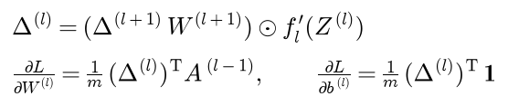
Only the taken action's output receives an error. The other outputs still change after the step, because they share the hidden layers.

Huber loss and gradient clipping

The Huber loss is quadratic for small errors and linear for large ones:

At |e| = κ both pieces equal κ²/2 and both slopes equal ±κ, so the loss is continuously differentiable. Its derivative is the error clipped to [-κ, κ]: a transition with a huge TD error, typically early in training or right after a target update, pushes no harder than one with error κ. The squared loss would let it dominate the batch. The original DQN clipped the error term of the squared loss to [-1, 1], which is the same thing as the Huber loss with κ = 1.

Clipping by global norm acts on the whole update instead. With g the gradient of all parameters stacked into one vector,

which keeps the direction and caps the length at c. The two are complementary: the Huber loss limits each transition's influence within a batch, the norm clip limits the size of the step.

Experience replay

The replay buffer holds the last N transitions in a circular array. Once it is full, each new transition overwrites the oldest. Every update draws m indices uniformly at random, with replacement, from the filled part.

Two properties make this work. First, sampling decorrelates the batch. Gradient descent assumes the examples of a batch are roughly independent draws from one distribution; consecutive transitions are neither independent nor representative, since they all come from the last moments of one episode. In a buffer of 5,000 CartPole transitions, the correlation of the pole angle between neighbouring rows of a batch of 128 is 0.947 for consecutive transitions and -0.043 for replayed ones; for the cart position it falls from 1.000 to 0.099. Second, each transition is reused in many updates: a buffer that receives one transition per update keeps each for N updates, each of which picks it with probability about m / N, so it is replayed about m times.

Replay is only valid for an off-policy method. The stored actions were chosen by older versions of the policy, and the Q-learning target does not care: its maximum evaluates the greedy policy whatever behaviour produced the transition. Methods whose targets follow the behaviour policy, such as multi-step returns or SARSA, need corrections when combined with replay.

Target networks: hard copies and soft updates

A hard update copies the online parameters into the target every C updates and leaves them fixed in between:

A soft update, or Polyak average, moves the target a fraction τ in (0, 1] of the way towards the online network after every update:

Unrolling the soft update over t steps shows that the target is an exponential moving average of past online parameters:

The weights τ(1 - τ)ᵏ form a geometric distribution over the age k of the parameters. Under a hard update the age is 0, 1, ..., C - 1 in turn. Setting the two mean ages equal gives a rule for translating between them:

A copy every 100 updates corresponds to τ = 2/101 ≈ 0.0198, and a copy every 50 to τ = 2/51 ≈ 0.0392. The two rules still differ in character:

• Between updates, a hard target is fixed for C updates and then jumps; a soft target changes a little after every update.
• With a hard target the learner solves a sequence of ordinary regression problems, one per copy; with a soft target it solves one regression problem whose targets drift slowly.
• A hard copy propagates value exactly one backup per copy; a soft update propagates it smoothly, about one backup per 1/τ updates.
• A hard update needs an update counter; a soft update needs no extra state.
• C = 1 means no target network at all, and τ = 1 is a copy after every update.
• In practice, DQN on discrete actions uses hard copies with C from hundreds to tens of thousands, and continuous control methods such as DDPG, TD3 and SAC use soft updates with τ from 0.001 to 0.05.

The copy period also limits how fast values can grow. With exact fitting, each copy performs one step of value iteration on the target, so with a reward of 1 per step the values after k copies have only reached the k-step value:

examples/target_networks.py trains the agent on CartPole cut at 20 steps, with γ = 0.95 and a copy every 500 updates. Its start-state values are 0.972, 1.922 and 8.180 after 1, 2 and 10 copies, against k-step values of 1, 1.95 and 8.0253: one backup per copy, with a little overestimation from the maximum on top by the end. Its values would need about 90 copies, 45,000 updates, to reach 99 % of their limit of 20. Long copy periods are safe but slow.

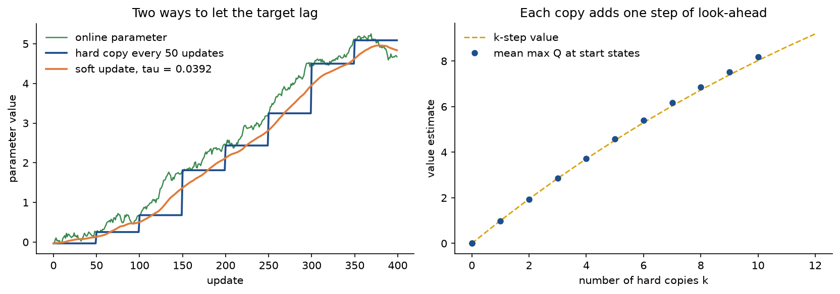
The left panel shows the two kinds of lag on a toy parameter path: both targets trail the online value by 24.5 updates on average, but one moves in steps and the other glides. The right panel shows the speed limit: the measured values climb along the k-step curve, one backup per copy.

Why does a target network help at all? Without one, the target of a transition contains the largest online value at s′, and because s′ resembles s, the update that raises Q(s, a) also raises the values at s′, so the target runs away from the estimate it is meant to pull. Function approximation, bootstrapping and off-policy data together are known as the deadly triad: any two are harmless, all three can diverge. The target network breaks the feedback loop for C updates at a time.

Terminated versus truncated

Since Gym 0.26, and in every Gymnasium release, step returns two end-of-episode flags instead of one:

• terminated is true when the environment reached a terminal state of the decision process. In CartPole the pole has fallen past 12 degrees or the cart has left the track. Nothing follows, so the value of what comes next is zero and the target is y = r.
• truncated is true when something outside the decision process stopped the episode, usually a time limit. CartPole-v1 ends every episode after 500 steps through the TimeLimit wrapper. The state at the cut is an ordinary state with a future the agent cannot see, so the target must still bootstrap from s′, the observation returned at the cut, before any reset.

Only terminated may enter the target as d. Treating terminated or truncated as terminal, as code written for the older single done flag does, biases every value downwards, by an amount that can be computed exactly in the simplest case. Take a process with one state, a reward r at every step and no terminal state, cut into episodes of T steps by a limit the learner cannot observe. The true value is r / (1 - γ). If the cut is treated as terminal, a fraction p = 1/T of the targets is r instead of r + γV. TD learning with the squared loss converges to the value at which the average error vanishes:

For γ = 0.9 and T = 10 that is 1/(1 - 0.81) = 5.2632 instead of 10. For CartPole-v1, with γ = 0.99 and T = 500, a policy that always survives would be valued at 83.4725 instead of 100, if the network could not read the elapsed time from the state.

With the Huber loss the average error is replaced by the average of clipped errors. When the majority errors lie inside κ and the cut errors outside, the balance condition becomes

which is (1 - 0.1111)/0.1 = 8.8889 for γ = 0.9, T = 10 and κ = 1. The Huber loss treats the rare cut targets as outliers and hides most of the bias. TD learning on the one-state process, run by examples/time_limits.py, settles at 9.9752, 5.2530 and 8.8504 for the three cases. The correct fixes are to bootstrap through truncations, or to put the remaining time into the observation so that the cut becomes a genuine terminal state of a larger, time-aware process.

Overestimation and double DQN

The target uses the maximum of noisy estimates. Because the maximum is a convex function, Jensen's inequality gives

with equality only when the noise never changes which action looks best. For k actions with equal true values and independent Gaussian errors of standard deviation σ, the bias is σ times the expected maximum of k standard normal variables:

That is 0.5642σ for two actions, 1.0294σ for four and 1.4236σ for eight. Bootstrapping then copies the inflated value into the targets of every earlier state.

The double estimator decouples choosing from evaluating. With two independent estimates A and B, it lets A pick the action and B report its value:

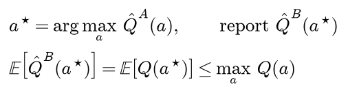
Since B is independent of the choice, the result is unbiased when the true values are equal, and slightly pessimistic otherwise. Double DQN uses the two networks it already has, the online network to choose and the target network to evaluate:

The fix is partial, because the target network is a lagged copy of the online network and their errors are correlated. examples/overestimation.py sets up a decision problem in which going on to a fork of eight noisy actions with mean reward -0.2 is worse than stopping with reward 0. Averaged over 2,000 runs of tabular learning, plain max targets make the agent choose the worse branch in 91.0 % of runs at the worst episode, double-DQN-style targets in 78.1 %, and two independent tables in at most 51.3 %, which is just the initial coin toss. With 10 % exploration the optimum is 5 %.

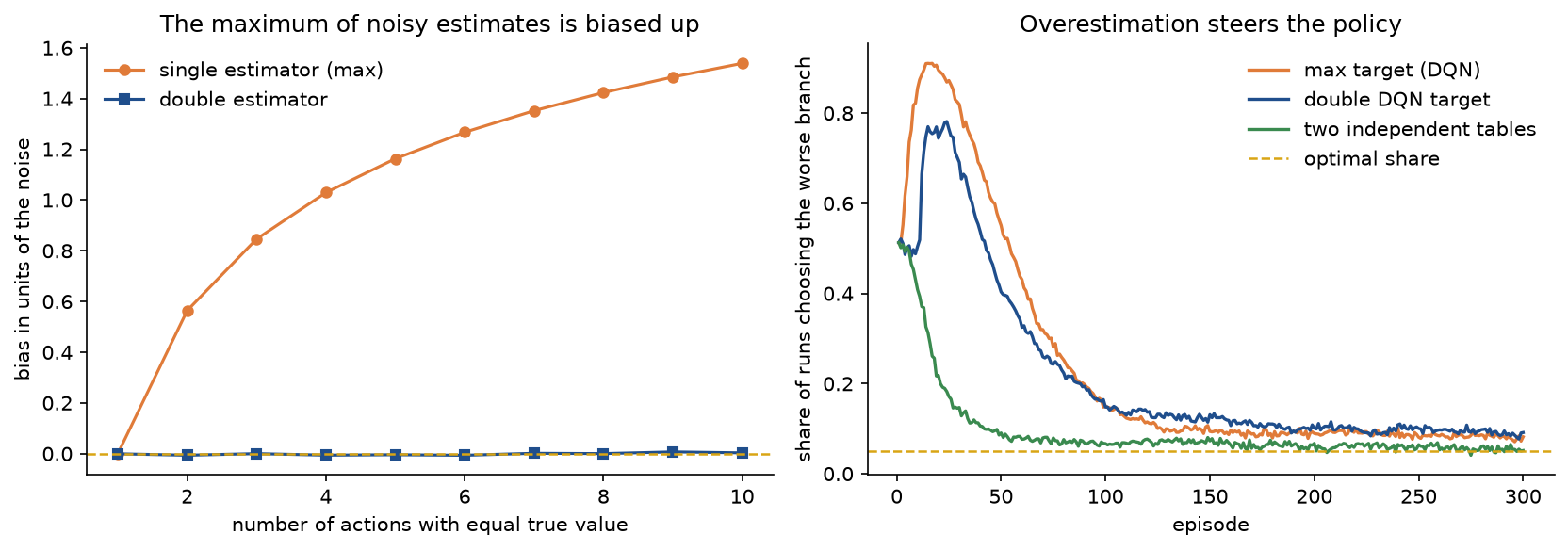
The left panel shows that the bias of the maximum grows with the number of actions while the double estimator has none. The right panel shows the bias steering behaviour: all three rules eventually learn to stop, but plain max targets first pull nearly every run towards the worse branch.

Exploration

The agent acts ε-greedily: with probability ε it picks an action uniformly at random, otherwise the action with the largest online value. A replay buffer full of transitions from a near-deterministic policy teaches nothing about the other actions, so ε starts at 1 and decays. Two common schedules over environment steps t, with start value ε₀, floor ε₁, duration T and decay factor ρ below 1:

The CartPole agent uses the linear schedule from 1 to 0.02 over 10,000 steps. The evaluation policy is greedy, with ε = 0.

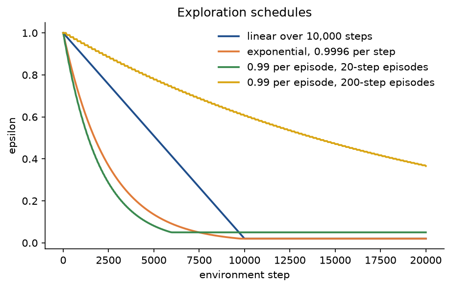
The figure, written by examples/replay_and_exploration.py, shows why the schedule must count environment steps: the same per-episode decay is ten times slower in steps when episodes are ten times longer, and episodes get longer exactly when the agent improves.

The algorithm

1. Initialize the online network θ randomly, set θ⁻ = θ, and create an empty buffer of capacity N.
2. Observe the first state s. For every environment step t = 1, 2, ...:
3. Choose a ε-greedily with respect to the online values at s and execute it; observe r, s′, terminated and truncated.
4. Store (s, a, r, s′, d) with d = terminated. If the episode ended for either reason, reset and observe a new s; otherwise set s to s′.
5. After a warm-up of a few thousand steps, sample a mini-batch of m transitions, compute the targets with θ⁻ (double or plain), the TD errors and the Huber loss, backpropagate, clip the global gradient norm to c and take an optimizer step on θ.
6. Update the target: copy θ into θ⁻ every C updates, or apply the Polyak average with τ after each one.

Worked example

A network with two inputs, three ReLU hidden units and two linear outputs, one per action, γ = 0.9, the Huber loss with κ = 1 and a mini-batch of m = 3 transitions. To keep the hand computation short, the target network shares the hidden layer of the online network and differs only in its output layer.

The diagram gives every parameter. As matrices, W1 has rows (0.5, -0.3), (0.2, 0.8) and (-0.6, 0.4), one row per hidden unit, and b1 is (0.1, 0.0, 0.2). The online output layer W2 has rows (1.0, -0.5, 0.3) and (-0.2, 0.7, 0.6), one row per action, with b2 = (0.0, 0.1); the target output layer has rows (0.8, -0.4, 0.7) and (0.0, 0.6, 0.4), with biases (0.1, 0.0). The batch, with actions numbered 0 and 1:

• Transition 1: state (1.0, 0.5), action 0, reward 0.5, next state (0.8, 1.0), neither terminated nor truncated.
• Transition 2: state (-0.5, 1.0), action 1, reward -1.0, next state (0.2, -0.5), terminated.
• Transition 3: state (0.4, -1.0), action 1, reward 0.2, next state (-1.0, 0.6), truncated by a time limit.

So d = (0, 1, 0): the third transition hit a time limit and still bootstraps. Every value below is computed in double precision and rounded to four decimals for display.

Forward pass

For transition 1 and hidden unit 1 the net input is 0.5 × 1.0 - 0.3 × 0.5 + 0.1 = 0.45. Applying the ReLU and the online output layer:

• Transition 1: hidden net inputs (0.45, 0.6, -0.2), activations (0.45, 0.6, 0), action values (0.15, 0.43).
• Transition 2: hidden net inputs (-0.45, 0.7, 0.9), activations (0, 0.7, 0.9), action values (-0.08, 1.13).
• Transition 3: hidden net inputs (0.6, -0.72, -0.44), activations (0.6, 0, 0), action values (0.6, -0.02).

For transition 1 and action 0, Q = 1.0 × 0.45 - 0.5 × 0.6 + 0.3 × 0 + 0.0 = 0.15. The values of the actions actually taken are (0.15, 1.13, -0.02).

Targets

The next states pass through the shared hidden layer, giving activations (0.2, 0.96, 0.12), (0.35, 0, 0) and (0, 0.28, 1.04). The two output layers then give:

• Online network at the next states: (-0.244, 0.804), (0.35, 0.03) and (0.172, 0.92).
• Target network at the next states: (-0.04, 0.624), (0.38, 0.0) and (0.716, 0.584).

The DQN targets use the largest target-network value of each row, except for the terminal transition: y1 = 0.5 + 0.9 × 0.624 = 1.0616, y2 = -1.0 and y3 = 0.2 + 0.9 × 0.716 = 0.8444. The TD errors are 0.15 - 1.0616 = -0.9116, 1.13 + 1.0 = 2.13 and -0.02 - 0.8444 = -0.8644. The network was too pessimistic about transitions 1 and 3 and far too optimistic about transition 2, whose episode ended with a penalty. Had the time limit of transition 3 been treated as terminal, its target would have been 0.2 and its error only -0.22.

Loss

Errors 1 and 3 lie inside κ = 1 and error 2 outside, so the per-transition losses are:

• Transition 1: one half of 0.9116 squared, 0.4155.
• Transition 2: 1 × (2.13 - 0.5) = 1.63.
• Transition 3: one half of 0.8644 squared, 0.3736.

The loss is their mean, (0.4155 + 1.63 + 0.3736) / 3 = 0.8064. With the squared loss, transition 2 alone would contribute 2.13² / 2 = 2.26845 and the loss would be 1.0192.

Backward pass

Each row of the output error Δ2 holds ψ(e), the error clipped to [-1, 1], in the column of the action taken, and zero in the other column. The second error is clipped from 2.13 to 1, so the rows of Δ2 are (-0.9116, 0), (0, 1) and (0, -0.8644).

The next equation sends each row back through W2 and multiplies by the ReLU derivative, which is 1 where the hidden net input is positive and 0 elsewhere. For transition 1, -0.9116 × (1.0, -0.5, 0.3) = (-0.9116, 0.4558, -0.2735), and the third hidden unit is inactive. For transition 3, -0.8644 × (-0.2, 0.7, 0.6) = (0.1729, -0.6051, -0.5186), and only the first hidden unit is active. The rows of Δ1 are therefore (-0.9116, 0.4558, 0), (0, 0.7, 0.6) and (0.1729, 0, 0).

Gradients

Averaged over the batch:

• Output layer: the gradient of W2 has rows (-0.1367, -0.1823, 0) and (-0.1729, 0.2333, 0.3), and the gradient of b2 is (-0.3039, 0.0452).
• Hidden layer: the gradient of W1 has rows (-0.2808, -0.2096), (0.0353, 0.3093) and (-0.1, 0.2), and the gradient of b1 is (-0.2462, 0.3853, 0.2).

Row 1 of the W2 gradient comes from transition 1 alone, the only one that took action 0: (-0.9116 / 3) × (0.45, 0.6, 0) = (-0.1367, -0.1823, 0). The top-left entry of the W1 gradient is (-0.9116 × 1.0 + 0 × (-0.5) + 0.1729 × 0.4) / 3 = -0.2808.

Clipping and the update

The global norm of the four gradient arrays, 17 numbers stacked into one vector, is 0.9162. Clipping to c = 0.5 multiplies every gradient by 0.5 / 0.9162 = 0.5457. A plain gradient step with η = 0.1 then gives:

• W1 with rows (0.5153, -0.2886), (0.1981, 0.7831) and (-0.5945, 0.3891), and b1 = (0.1134, -0.0210, 0.1891).
• W2 with rows (1.0075, -0.4901, 0.3) and (-0.1906, 0.6873, 0.5836), and b2 = (0.0166, 0.0975).

With the same targets the loss falls from 0.8064 to 0.7618. The target network has not changed, so the targets really are the same.

Double DQN targets

The online network prefers actions (1, 0, 1) at the next states and the target network (1, 0, 0). They disagree on transition 3: the plain target bootstraps from the target network's own favourite, 0.716, whereas double DQN evaluates the online network's choice, action 1, with the target network: y3 = 0.2 + 0.9 × 0.584 = 0.7256, and the error becomes -0.7456. Transitions 1 and 2 keep their targets, and the loss becomes 0.7745. The double target is never larger than the plain one, since it evaluates one action with the network whose maximum the plain target takes.

Target update

A hard copy makes θ⁻ equal to the updated online parameters. A soft update with τ = 0.1 moves it a tenth of the way, in both layers; the target output layer becomes rows (0.8207, -0.4090, 0.6600) and (-0.0191, 0.6087, 0.4184) with biases (0.0917, 0.0098). For instance the first bias is 0.1 × 0.0166 + 0.9 × 0.1 = 0.0917.

Two cross-checks. PyTorch's autograd, applied to the same loss on double-precision copies of the networks, reproduces every gradient to within 6 × 10⁻¹⁷ for both losses and both targets, and a central-difference check of the semi-gradient with the targets held fixed gives relative errors of about 10⁻¹⁰. Every value of the update in this section is asserted by tests/test_trace.py and printed by examples/worked_update.py; the two cross-checks are asserted by tests/test_comparisons.py and tests/test_update.py.

The code

The package deep_q_networks has a NumPy half for everything that can be checked by hand and a PyTorch half for the agent. PyTorch and Gymnasium are imported inside the functions that need them, so the NumPy half works without either.

• arrays.py holds the array types and as_matrix, which insists on one transition per row.
• network.py holds the frozen QNetwork with ReLU hidden layers and a linear output per action, its forward, q_values and parameters, and initialize_q_network.
• replay.py holds Batch, make_batch and ReplayBuffer, a seeded circular buffer of NumPy arrays with add, sample and chronological_indices.
• targets.py holds td_targets and double_td_targets.
• losses.py holds the Huber and squared losses with their derivatives, collected in LOSSES.
• update.py is the heart of the topic: dqn_loss_trace computes the targets, errors, losses, output error and backpropagated gradients of one batch, and clip_by_global_norm and sgd_step finish the update.
• trace.py holds the worked example, trace_update, which keeps every value of one update, and format_loss_trace, which prints them.
• gradient_check.py holds the finite-difference check of the semi-gradient and the random problem the tests use.
• target_networks.py holds soft_update, hard_update, track_target, mean_target_lag, matching_tau and value_after_copies.
• exploration.py, time_limits.py and overestimation.py hold the schedules, the exact and simulated time-limit bias, and the estimator experiments.
• tables.py, measurements.py and cartpole.py hold the table coverage count, smoothing, correlations and discounted returns, and the CartPole helpers: the balancing rule, the random policy, a noisy data collector, start states and evaluate_policy, which plays one episode per seed in lockstep.
• torch_networks.py and torch_update.py hold the PyTorch network, conversions to and from QNetwork, the greedy policy, and the agent's loss, clipping and Polyak update written out.
• agent.py holds DQNConfig and DQNAgent; training.py holds train_dqn, which pins one thread, trains, validates at checkpoints and keeps the best network; checkpoints.py saves and loads trained networks.
• comparisons.py checks our update and helpers against autograd, huber_loss, smooth_l1_loss, clip_grad_norm_ and lerp_.
• plotting.py and training_plots.py draw every figure in the handbook's four colours.

dqn_loss_trace is the mini-batch form of the equations above. The only lines that differ from a supervised network are the targets and the output error, which is nonzero only in the column of the action taken:

errors = chosen_q - targets
losses = chosen_loss.per_example(errors, kappa)
delta = np.zeros_like(q_values)
delta[rows, batch.actions] = chosen_loss.derivative(errors, kappa)

The agent's loss in PyTorch computes the targets under torch.no_grad(), which is what makes it a semi-gradient, and the training loop stores only terminated as the terminal flag, with the next observation taken before any reset. The flag time_limit_as_terminal exists only to reproduce the bug:

next_observation, reward, terminated, truncated, _ = env.step(action)
stored_terminal = terminated or (truncated and config.time_limit_as_terminal)
agent.remember(observation, action, float(reward), next_observation, stored_terminal)

The examples and the project import the package, so install the repository first as described in the main README. Each example demonstrates one idea and runs from the repository root:

• examples/worked_update.py prints every value of the worked example in the order above, then the squared-loss losses, the update, the double DQN targets and the target updates.
• examples/replay_and_exploration.py counts the table coverage, measures the correlation of consecutive and replayed batches, shows what a per-episode epsilon decay does and saves the exploration figure.
• examples/target_networks.py compares the lag of hard and soft targets and runs the copy-limited CartPole training, in about ten seconds.
• examples/time_limits.py computes the time-limit bias exactly and in four CartPole runs, in about half a minute.
• examples/overestimation.py measures the bias of the single and double estimators and runs the decision problem.
• examples/compare_with_pytorch.py compares our gradients with autograd and our helpers with PyTorch's built-ins, shows the gradient through the target, and saves the Huber loss figure.

python reinforcement-learning/deep-q-networks/examples/worked_update.py
python reinforcement-learning/deep-q-networks/examples/replay_and_exploration.py
python reinforcement-learning/deep-q-networks/examples/target_networks.py
python reinforcement-learning/deep-q-networks/examples/time_limits.py
python reinforcement-learning/deep-q-networks/examples/overestimation.py
python reinforcement-learning/deep-q-networks/examples/compare_with_pytorch.py

The sample project, project/cartpole_agent.py, trains a complete agent on CartPole-v1 and evaluates it the way an agent should be evaluated. CartPole-v1 gives a reward of 1 for every step, including the step on which the pole falls, terminates when the pole leans more than 12 degrees or the cart leaves the track, and truncates after 500 steps, so 500 is the largest return. The agent has a 4-128-128-2 network, Adam with learning rate 0.00025 (see Optimizers), γ = 0.99, a buffer of 50,000 transitions, mini-batches of 128, one update per environment step after 1,000 warm-up steps, ε falling linearly from 1 to 0.02 over 10,000 steps, a hard copy every 100 updates, double DQN targets, the Huber loss with κ = 1 and the global gradient norm clipped at 10. It trains for 40,000 environment steps with seed 0.

The evaluation protocol separates four roles. Training uses seed 0. Model selection uses 10 validation seeds, played every 2,000 steps with the greedy policy, and keeps the checkpoint with the best mean. Reporting uses 50 test seeds, disjoint from both, played once at the end. The value estimates are probed at the start states of 64 further seeds. The selected network is saved to the path given by --checkpoint, by default .data/deep-q-networks/cartpole-dqn.pt at the repository root, which git ignores, then loaded back, and the loaded copy is the one evaluated. Options switch the target update between --target-update hard with --target-period and --target-update soft with --tau (by default 2/(C + 1)), and change --steps, --seed, --loss, --learning-rate, --gamma and --hidden; --no-double uses plain targets, --time-limit-as-terminal reproduces the bug, --evaluate-only evaluates a saved checkpoint without training, and --figures sends the two PNGs to another folder. The default run takes about 40 seconds on one thread and stays under 400 MB of memory.

python reinforcement-learning/deep-q-networks/project/cartpole_agent.py
python reinforcement-learning/deep-q-networks/project/cartpole_agent.py --evaluate-only
python reinforcement-learning/deep-q-networks/project/cartpole_agent.py --target-update soft \
    --checkpoint .data/deep-q-networks/soft.pt --figures soft-run-figures

With the defaults, training takes 313 episodes, of which 294 terminated and 19 were cut by the time limit and bootstrapped; exactly 294 transitions are stored as terminal. The greedy policy scores 179.1 on the validation seeds at step 2,000, first reaches 500.0 at step 14,000, falls back to 120.7 at step 22,000, holds 500.0 from step 32,000 to 38,000 and drops to 141.2 at step 40,000. The best checkpoint is the one at step 38,000. On the 50 test seeds:

• The random policy has a mean return of 21.5 (standard deviation 13.7, minimum 10) and never reaches 500.
• The balancing rule, push towards the side the pole is falling to when the angle plus half the angular velocity is positive, reaches 500 on every seed.
• The network at the end of training has a mean of 135.9 (standard deviation 4.1, minimum 129) and never reaches 500.
• The network selected on the validation seeds reaches 500 on every seed.

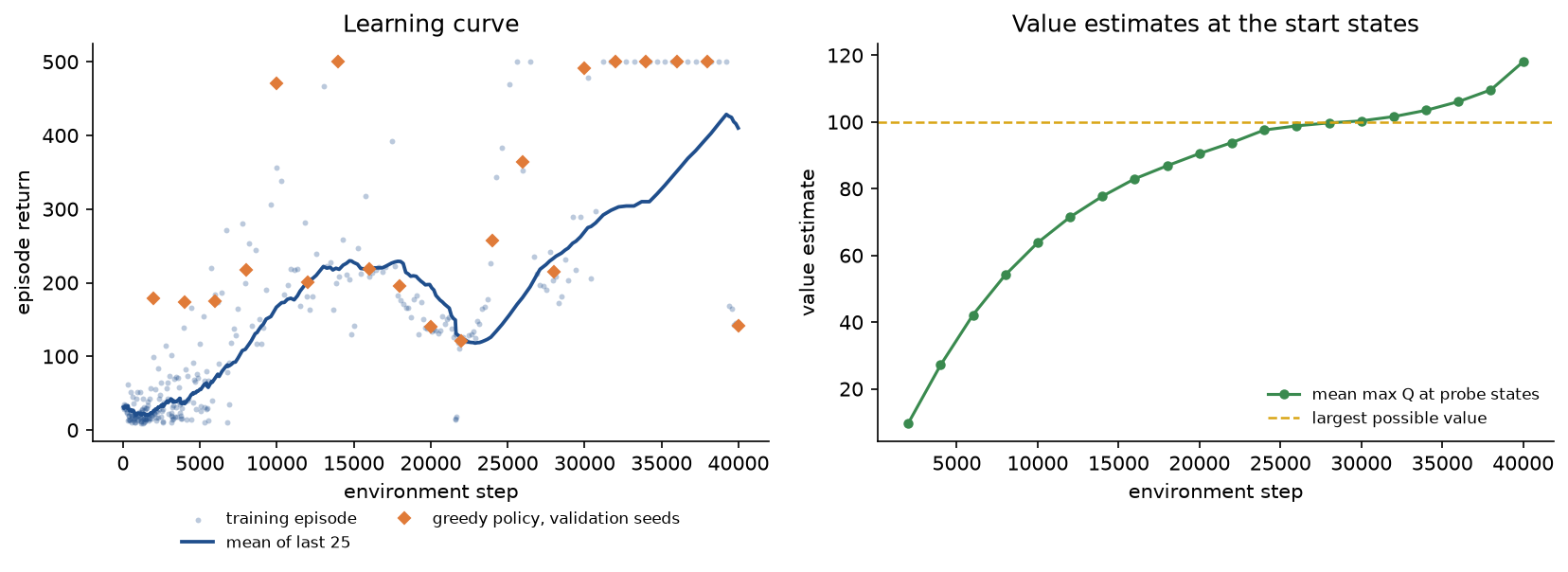
The left panel shows how unstable DQN on CartPole is: the greedy policy reaches 500, loses it and recovers, and the last checkpoint is far from the best. The right panel shows the value estimates at the probe states. They rise roughly like the k-step value of the copies made so far, pass 100, which no policy can earn with γ = 0.99, near step 30,000, and reach 118.0 at the end.

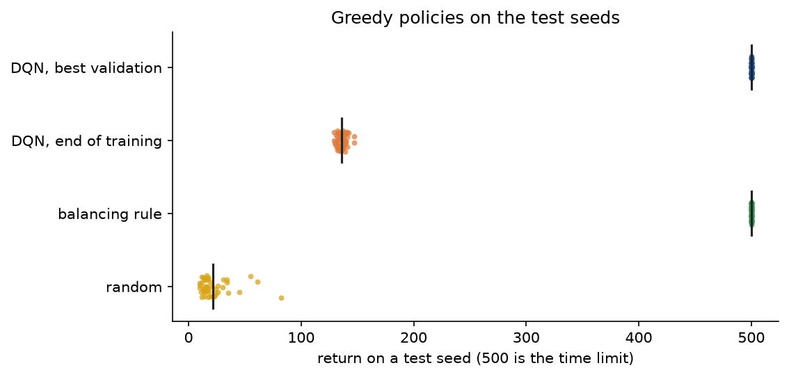
The selected network balances on every test seed; the final one does not, a reminder that the last checkpoint of a DQN run is not necessarily its best and that selection must not use the test seeds. The selected network predicts a mean largest action value of 109.7 at the 50 test start states, while the discounted return it actually earns there is:

an overestimate of about 10 %, even with double DQN targets. One training seed is a demonstration, not a measurement. Comparing two configurations needs several training seeds and intervals over them, as Honest evaluation discusses.

The notebook deep_q_networks.ipynb is a guided tour in the order of this page: the table coverage, the worked example through trace_update and again in bare NumPy, autograd, replay correlations, hard and soft targets with the copy-limited value growth, the overestimation experiments, the exploration and loss plots, one cell per pitfall below, the same CartPole run as the project with its evaluation, and the PyTorch built-ins. It runs in about a minute on one thread, most of it in the CartPole training cell. The tests in tests check the worked example value by value, the mathematical properties above, the agreement with PyTorch and the training loop's bookkeeping, and run in a few seconds:

python -m pytest reinforcement-learning/deep-q-networks

No dataset is involved. CartPole-v1 is a simulator shipped with Gymnasium under the MIT licence, the other examples are generated from seeds, and trained weights are written only to the ignored .data folder.

In practice

The agent writes out its own Huber loss, clipping and Polyak update so that each step is visible. PyTorch has all three, and examples/compare_with_pytorch.py confirms that they agree with ours:

• torch.nn.functional.huber_loss(q, y, delta=kappa) equals our Huber loss exactly.
• torch.nn.functional.smooth_l1_loss(q, y, beta=kappa) equals the Huber loss divided by κ; multiplied by κ it agrees exactly, and as it is it differs by up to 2.0 for κ = 2 on errors in [-3, 3].
• torch.nn.utils.clip_grad_norm_(parameters, max_norm) reports the same norm, 0.9162 on the worked example, and its clipped gradient differs from ours by at most 3 × 10⁻¹⁷.
• target_parameter.lerp_(online_parameter, tau) for each parameter is a soft update, within 1.1 × 10⁻¹⁶ of ours.
• Autograd on our loss reproduces the hand-derived gradient to within 1.1 × 10⁻¹⁶ on the worked example and on a random 3-6-5-2 network, for both losses and both targets.

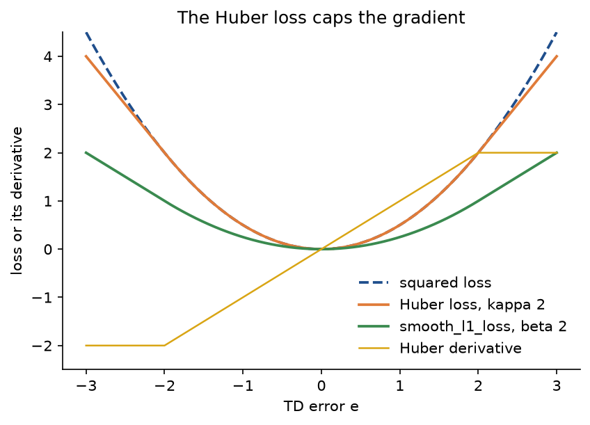
The figure shows why the two library losses are easy to confuse: with κ = 1 they coincide, but with any other threshold smooth L1 is the Huber loss scaled by 1/κ, and so is its gradient.

Mature implementations exist and should be preferred for anything beyond learning. None of them is a dependency of this repository.

• Stable-Baselines3 provides DQN("MlpPolicy", env). It uses the smooth L1 loss, clips the gradient norm at 10 by default, and implements target updates as a Polyak average applied every target_update_interval steps, so its default tau=1.0 is a hard copy. Its replay buffer bootstraps through time limits by default (handle_timeout_termination=True). It implements plain DQN targets, not double DQN.
• CleanRL has a single-file dqn.py that is easy to read side by side with this package.
• TorchRL offers composable losses (DQNLoss with a double_dqn option), replay buffers and target updaters for larger projects.

When to use which: the from-scratch agent to understand every line and to experiment with one change at a time; a library for baselines, many seeds, vectorized environments and logging. Whatever the implementation, check how it treats truncation, which target update it performs and what its tau means.

DQN is the base of a family of value-based methods for discrete actions. Each of the following changes one part of it and can be added to this agent.

• Dueling networks split the head into a state value and action advantages, so the state value is learned from every transition, whichever action was taken, which helps when many actions have similar values:

Subtracting the mean advantage makes the split unique.

• Prioritized experience replay samples surprising transitions more often and corrects the resulting bias with importance weights:

With α = 0 it is uniform replay again.

• Multi-step targets propagate rewards n steps per update, at the price of a small off-policy bias:

With n = 1 it is the ordinary DQN target.

• Distributional methods (C51, QR-DQN) learn the whole distribution of returns instead of its mean, and noisy networks replace ε-greedy exploration with learned parameter noise.
• Rainbow combines double DQN, prioritized replay, dueling heads, multi-step targets, distributional learning and noisy networks, and showed that the gains largely add up on Atari games.

For continuous actions the maximum over actions is no longer a lookup, and actor-critic methods such as DDPG, TD3 and SAC take over, with the same replay buffers and soft target updates. Learning-based navigation and Game-playing agents build on these ideas.

Pitfalls

• Treating the time limit as terminal. done = terminated or truncated cuts the bootstrap at every time limit and biases all values downwards: to 5.2632 instead of 10 in the one-state process with γ = 0.9 and T = 10, and to 83.4725 instead of 100 for a CartPole-v1 policy that always survives, if time is invisible. In examples/time_limits.py, CartPole with a 20-step limit and γ = 0.95 gives start-state values of 21.29 when bootstrapping and 11.95 when cutting, with the squared loss. The formula's 10.2564 assumes the elapsed time is invisible and the 20-step value 12.8303 assumes it is perfectly visible; the cut run lands between the two, because the network partly reads the time from the state, for example from how far the cart has drifted. The bootstrapping run overshoots the true value of 20 a little, the overestimation of the maximum. With the Huber loss the cut run reaches 19.52 against 20.46: the robust loss hides most of the bias, which is luck rather than a fix. Store terminated only, and with vector environments that reset automatically, take s′ from the final observation of the finished episode, not the first observation of the next one.

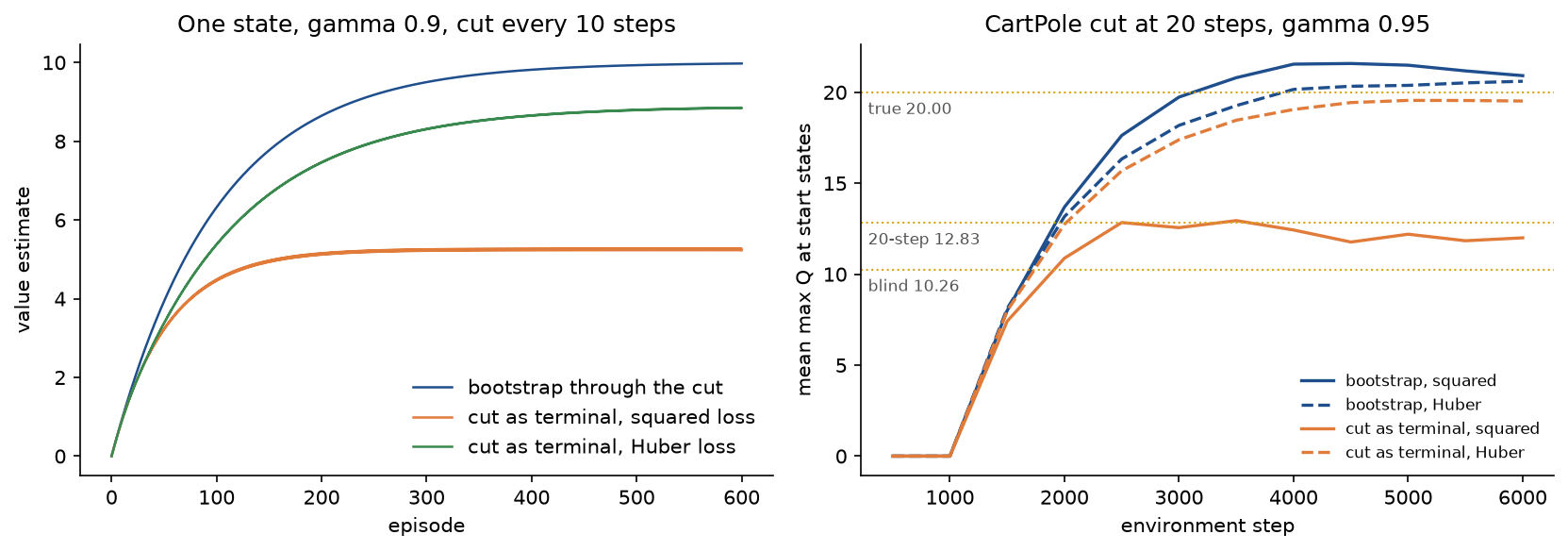
The left panel matches the fixed points derived under How it works; the right panel shows the same bias inside the agent, where only the squared-loss run reveals its full size.

• Letting the gradient flow through the target. Computing y with the online network outside torch.no_grad(), or forgetting .detach(), differentiates the target too and changes the update entirely. On the worked example with the online network computing its own targets, the top row of the W1 gradient is (-0.3067, -0.2333) as a semi-gradient and (-0.3547, -0.2933) through the target, and the middle row changes from (0.0500, 0.3167) to (0.0080, 0.6527). examples/compare_with_pytorch.py prints both.
• Describing one target update and implementing another. A hard copy every C updates and a soft update with τ are different algorithms, and their hyperparameters do not transfer by eye: a copy every 100 updates corresponds to τ = 2/101 ≈ 0.0198 in mean lag, not to τ = 0.01 or 0.1. Code that says "copy the target every N steps" in its documentation and applies a Polyak average in its loop, or the reverse, gives results nobody can reproduce from the description. Say which rule is used and with which constant.
• Reading τ the wrong way round. Here, as in most papers, τ is the weight of the online network. Some code bases write the update with the weight of the old target. Plugging 0.98 meant in that convention into ours gives a mean lag of 0.02 updates instead of 49: no target network at all. examples/target_networks.py prints both.
• A copy period too long for the budget. Each hard copy adds one backup. With γ = 0.95 and a copy every 500 updates, the start-state values in examples/target_networks.py are only 8.180 after 10 copies, against a limit of 20. With γ = 0.99 the values need hundreds of copies to approach 1/(1 - γ). Divide the budget by C and compare with the horizon 1/(1 - γ) before choosing C.
• Decaying ε once per episode. The schedule then depends on how long episodes last, which changes as the agent improves. A decay of 0.99 per episode reaches 0.05 after 299 episodes, which is 5,980 steps with 20-step episodes and 149,500 steps with 500-step ones. Decay per environment step.
• Confusing Huber and smooth L1. torch.nn.functional.smooth_l1_loss(q, y, beta=kappa) equals the Huber loss divided by κ. The two agree only for κ = 1; with another threshold the gradient, and so the effective learning rate, differs by a factor of κ, as the figure under In practice shows.
• Ignoring value estimates above the possible maximum. With rewards between 0 and some largest reward, no value can exceed that reward divided by 1 - γ. The project's run reaches 118.0 against a ceiling of 100 by its last checkpoint, a clear overestimate. Estimates in the hundreds or thousands mean divergence, and a lower learning rate, a longer copy period or double DQN targets are the usual remedies. Log the mean of the largest action value on a fixed set of probe states; it costs one forward pass.
• Reporting the training curve, the best episode or the last checkpoint. The training curve includes exploration, the best episode is selected after the fact, and the last checkpoint of an unstable run can be much worse than an earlier one: here 135.9 at the end against 500.0 for the checkpoint selected on validation seeds. Select on validation seeds, report on separate test seeds with the greedy policy, and use several training seeds before claiming that one setting beats another.
• Taking CartPole as evidence of capability. The one-line balancing rule balances for 500 steps on all 50 test seeds. CartPole is a smoke test that shows an implementation works, not a benchmark that separates good methods from bad ones.

Further reading

• V. Mnih et al., "Playing Atari with deep reinforcement learning", arXiv:1312.5602, 2013. The first DQN paper.
• V. Mnih et al., "Human-level control through deep reinforcement learning", Nature 518, 529-533, 2015. DQN with the target network and error clipping.
• L.-J. Lin, "Self-improving reactive agents based on reinforcement learning, planning and teaching", Machine Learning 8, 293-321, 1992. Experience replay.
• M. Riedmiller, "Neural fitted Q iteration: first experiences with a data efficient neural reinforcement learning method", ECML 2005.
• S. Thrun and A. Schwartz, "Issues in using function approximation for reinforcement learning", Proceedings of the Connectionist Models Summer School, 1993. Overestimation from the maximum.
• H. van Hasselt, "Double Q-learning", NeurIPS 2010.
• H. van Hasselt, A. Guez and D. Silver, "Deep reinforcement learning with double Q-learning", AAAI 2016.
• F. Pardo, A. Tavakoli, V. Levdik and P. Kormushev, "Time limits in reinforcement learning", ICML 2018.
• T. P. Lillicrap et al., "Continuous control with deep reinforcement learning", ICLR 2016. Soft target updates.
• Z. Wang et al., "Dueling network architectures for deep reinforcement learning", ICML 2016.
• T. Schaul, J. Quan, I. Antonoglou and D. Silver, "Prioritized experience replay", ICLR 2016.
• M. Hessel et al., "Rainbow: combining improvements in deep reinforcement learning", AAAI 2018.
• H. van Hasselt et al., "Deep reinforcement learning and the deadly triad", arXiv:1812.02648, 2018.
• R. S. Sutton and A. G. Barto, Reinforcement Learning: An Introduction, second edition, MIT Press, 2018. Section 6.7 on maximization bias and chapter 11 on the deadly triad.
• A. G. Barto, R. S. Sutton and C. W. Anderson, "Neuronlike adaptive elements that can solve difficult learning control problems", IEEE Transactions on Systems, Man, and Cybernetics 13(5), 834-846, 1983. The cart-pole task.
• P. Henderson et al., "Deep reinforcement learning that matters", AAAI 2018, and R. Agarwal et al., "Deep reinforcement learning at the edge of the statistical precipice", NeurIPS 2021. How to evaluate and compare agents.
• M. Towers et al., "Gymnasium: a standard interface for reinforcement learning environments", arXiv:2407.17032, 2024.