JPEG from scratch

A photograph stored as raw 8-bit RGB costs 24 bits per pixel, yet a JPEG file of the same picture usually needs one or two, and the difference is hard to see. Baseline JPEG gets there with a short chain of steps, each of which either exposes redundancy or throws away detail the eye barely notices: a change of colour space, coarser colour planes, a discrete cosine transform on 8x8 blocks, quantization, a zigzag scan and entropy coding. This page derives every step, follows one 8x8 block through the encoder and back through the decoder with every intermediate number shown, builds an encoder and decoder in NumPy that write and read real JFIF files, and measures rate against quality for a synthetic scene and a photograph next to Pillow's encoder. Afterwards you will be able to compute a JPEG block by hand, count its bits exactly, explain where blocking and ringing come from, and read the rate and quality numbers of any image codec critically. The Huffman codes at the end of the chain are treated in general in Entropy coding.

To run the code in this topic, install the base and vision groups, and the signal group for the comparison with SciPy's DCT.

Intuition

Neighbouring pixels in a natural image are strongly correlated: most of an 8x8 patch is a smooth brightness level plus a gentle slope, and only edges and texture add fine detail. Writing every pixel with 8 bits spends the same effort on the predictable part as on the detail. A good transform rotates the 64 pixel values into 64 coefficients so that a few low-frequency coefficients carry nearly all the energy and the rest are close to zero. The discrete cosine transform (DCT) does this almost as well as the best transform fitted to the image itself, and it is fixed, fast and the same for every image.

Once the energy sits in a few coefficients, two further facts save most of the bits. The eye is less sensitive to fine detail than to coarse structure, and less sensitive to colour detail than to brightness detail. So each coefficient is rounded to a multiple of a step size that grows with frequency, and the colour information is stored at half resolution in both directions. Most high-frequency coefficients become exactly zero. The zigzag scan lines the coefficients up from low to high frequency so that the zeros form long runs at the end, and a Huffman code gives short codewords to the common events: small values, short runs and the end of a block.

Only three things lose information: halving the colour resolution, rounding the coefficients, and rounding the decoded samples back to integers. The colour transform and the DCT are invertible, and the scan and the entropy code are exactly reversible. The visible artefacts follow from the lossy steps. When a block keeps little more than its average, it becomes a flat tile (blocking); when the high frequencies of a sharp edge are rounded away, the reconstruction oscillates next to the edge (ringing); and colour edges smear because the colour planes were coarser to begin with.

The diagram shows the encoder on the top row and the decoder, which undoes each step in reverse order, on the bottom row. The amber steps are the only ones that lose information; every blue step can be undone exactly or to rounding error.

How it works

Notation

The quantities below appear throughout. The formula images write subscripts such as C with a subscript b, or K with a subscript R; in the text these are simply Cb, Cr, KR and KB.

• R, G and B are the colour components of a pixel, integers from 0 to 255. Y is luma, Cb and Cr are the blue-difference and red-difference chroma components.
• KR = 0.299 and KB = 0.114 are the luma weights of red and blue, and KG = 1 - KR - KB = 0.587.
• N is the block size, 8. The sample in row i and column j of a block after the level shift is f(i, j), with i and j from 0 to N - 1.
• F(u, v) is a DCT coefficient. The first index u is the vertical frequency (the row of the coefficient block) and v the horizontal frequency (the column). The normalization c(k) is 1/√2 for k = 0 and 1 otherwise, and T is the N x N DCT matrix.
• Q(u, v) is the quantization step of coefficient (u, v), q is the quality setting from 1 to 100 and s(q) the table scale it implies, in percent. F̂(u, v) is the quantized coefficient, an integer, and F̃(u, v) the value the decoder rebuilds from it.
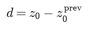
• z0 to z63 are the quantized coefficients in zigzag order, with z0 the DC coefficient. d is the difference between the DC coefficient of a block and that of the previous block of the same component.
• m(x) is the magnitude category of an integer x, the number of bits of its absolute value, and r is the number of zero coefficients before a nonzero one in zigzag order.

Colour transform

Luma is a weighted sum of the three components, with weights that roughly follow the eye's sensitivity to each:

The two colour differences B - Y and R - Y carry what luma leaves out. Since B - Y = (1 - KB) B - KR R - KG G, it ranges over plus or minus (1 - KB) times 255. Dividing by 2 (1 - KB) squeezes that range into plus or minus 127.5, and adding 128 makes it a valid 8-bit value. The same argument applies to red:

Expanding Y gives the matrix used by JFIF, the file format that carries almost every JPEG image:

The luma row sums to 1 and the chroma rows sum to 0, so a grey pixel, with R = G = B, has Cb = Cr = 128, and adding the same amount to all three components changes only Y. Inverting the two difference equations and then solving the luma equation for G gives the decoder's side:

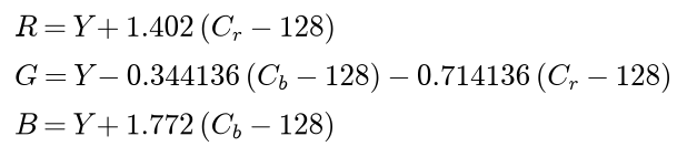
These are the full-range equations of JFIF. Standard-definition video (ITU-R BT.601) uses the same weights but limits luma to 16 to 235 and chroma to 16 to 240, and high-definition video uses different weights. Digital images and colour covers colour spaces in general.

Chroma subsampling

4:2:0 subsampling halves each chroma plane in both directions by averaging every 2x2 cell of samples C into one sample C′:

A pixel then costs one luma sample and a quarter of each chroma sample, 1 + 2 × 1/4 = 1.5 samples instead of 3, so the raw data halves before any coding starts. The averaged sample sits at the centre of its 2x2 cell. The decoder brings the plane back either by repeating each sample ("nearest") or, as libjpeg does by default, by linear interpolation at the centred positions. Along each axis an output sample lies a quarter of a chroma sample from its nearest chroma sample and three quarters from the next one, which gives the weights

applied to rows and then to columns, with the edge samples repeated. Other schemes are 4:4:4 (no subsampling) and 4:2:2 (horizontal only). The scheme works because natural images keep their detail in luma.

In the crop the wood grain and the rim of the cup are sharp in the luma plane, while the two chroma planes are smooth washes with little structure. That is why halving their resolution costs so little on photographs, and why it costs much more on graphics with saturated colour edges.

Level shift, blocks and padding

Each plane is cut into 8x8 blocks and 128 is subtracted from every sample, so that values lie in the range -128 to 127 and a mid-grey block has a DC coefficient of zero. With 4:2:0 the coding unit is a macroblock, also called the minimum coded unit, of 16x16 pixels: four luma blocks and one block of each chroma plane.

The diagram follows one macroblock: six blocks come out of 256 pixels, and they enter the scan in the order shown. An image whose size is not a multiple of the macroblock is padded by repeating its last row and column, and the decoder crops the padding away; the image is never stretched.

The two-dimensional DCT

The DCT-II of an N x N block, its inverse and the normalization are

For N = 8 the factor 2/N is the 1/4 found in many references; it is not 1/4 for other block sizes. The double sum factorizes. Define the matrix T and the row weights α:

The identity on the second line holds case by case: when u and v are both zero the product is 1/N = (2/N) × 1/2, when exactly one is zero it is √2/N = (2/N) × 1/√2, and otherwise it is 2/N. Substituting it into the definition turns the double sum into two matrix products:

The inner sum transforms every row of the block and the outer sum every column, so the 2-D DCT is two passes of the 1-D DCT: 2N³ = 1024 multiplications per block instead of N⁴ = 4096 for the direct sum. The rows of T are orthonormal, because the cosines of different frequencies cancel over the N sample positions and the squared cosines add up to N/2 (or N for the constant row), which α normalizes to 1:

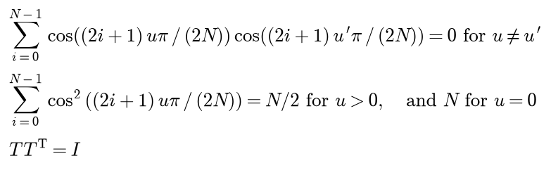
Three consequences follow from T Tᵀ = I:

• The inverse is f = Tᵀ F T, already shown above.
• Energy is preserved (Parseval), because multiplying by an orthogonal matrix on both sides preserves the sum of squares.
• The DC coefficient is N times the block mean, eight times for an 8x8 block.

Writing t(u) for row u of T, the inverse reads

so every block is a weighted sum of the 64 basis images formed by the outer products of two rows of T, and the coefficients are the weights.

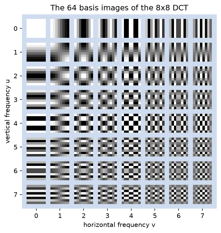
The image in row u of the grid varies u half periods from top to bottom, the one in column v varies v half periods from left to right. A smooth block needs only the images near the top left corner, which is the whole point of the transform.

Why the DCT concentrates energy

The transform that packs the most energy of a given set of blocks into the fewest coefficients is the Karhunen-Loeve transform (KLT): the eigenvectors of the blocks' second-moment matrix, ordered by eigenvalue. It is the same computation as PCA (Dimensionality reduction) and must be fitted to each image and sent with it. For blocks whose pixels follow a first-order Markov model with neighbour correlation close to 1, a reasonable model of natural images, the KLT basis tends to the DCT basis, so the fixed DCT is nearly optimal without any fitting.

A second view explains why the cosine transform beats the Fourier transform. Any transform of a finite block behaves as if the block were extended. The DFT extends it periodically, so a ramp jumps from its last value back to its first, and the jump needs every frequency to describe. The DCT-II corresponds to extending the block by its mirror image, which joins the ends continuously. Take the ramp -35, -25, ..., 35, whose energy is 4200:

• The orthonormal DCT magnitudes are 0, 64.4232, 0, 6.7345, 0, 2.0090, 0 and 0.5070, which leaves 1.18 % of the energy outside the first AC coefficient.
• The orthonormal DFT magnitudes are 0, 36.9552, 20, 15.3073, 14.1421, 15.3073, 20 and 36.9552, which leaves 34.97 % outside the lowest frequency pair.

On the photograph used below, the DC coefficient holds 91.09 % of the energy of the luma blocks. Of the remaining AC energy, the best 5 of 63 DCT coefficients capture 59.33 %, the KLT fitted to that very image 60.93 %, and the 5 strongest pixels only 11.18 %.

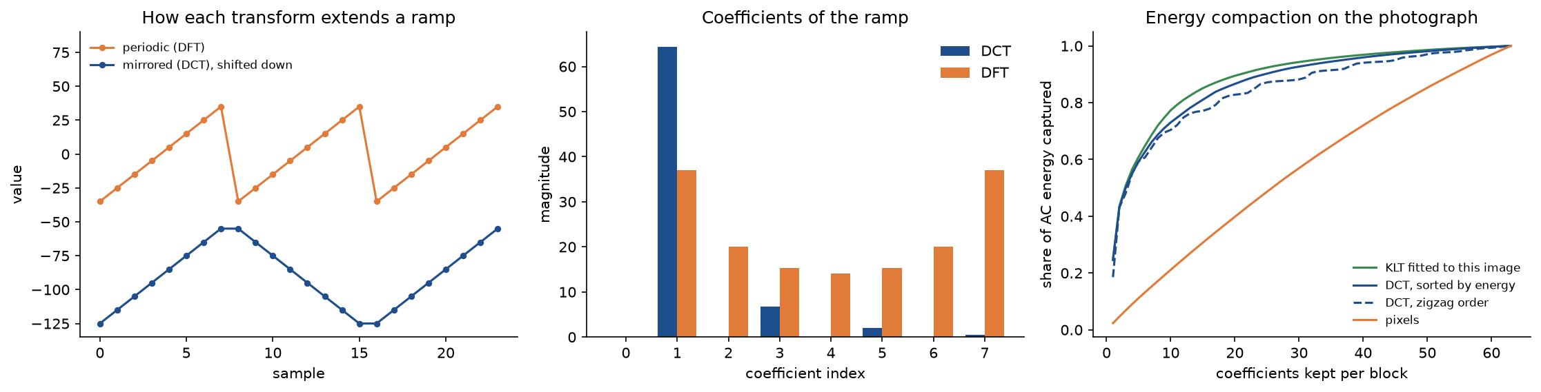
The right panel is the real argument for the DCT: a fixed basis, chosen without looking at the image, comes within a few per cent of the optimal basis fitted to it, and the zigzag order, which also ignores the image, is close to the best possible order.

Quantization

Each coefficient is divided by its step and rounded to the nearest integer, half away from zero, and the decoder multiplies back:

The error of each coefficient is at most half a step, and every coefficient whose magnitude is below half a step becomes zero. Because T is orthogonal, the mean squared error of the reconstructed block before the final rounding, with f̃ the reconstructed samples, equals the mean squared error of its coefficients, so distortion can be predicted and controlled in the coefficient domain:

The standard tables, published with the JPEG standard as examples derived from visibility experiments, have small steps at low frequencies and large steps at high frequencies, and much larger steps for chroma.

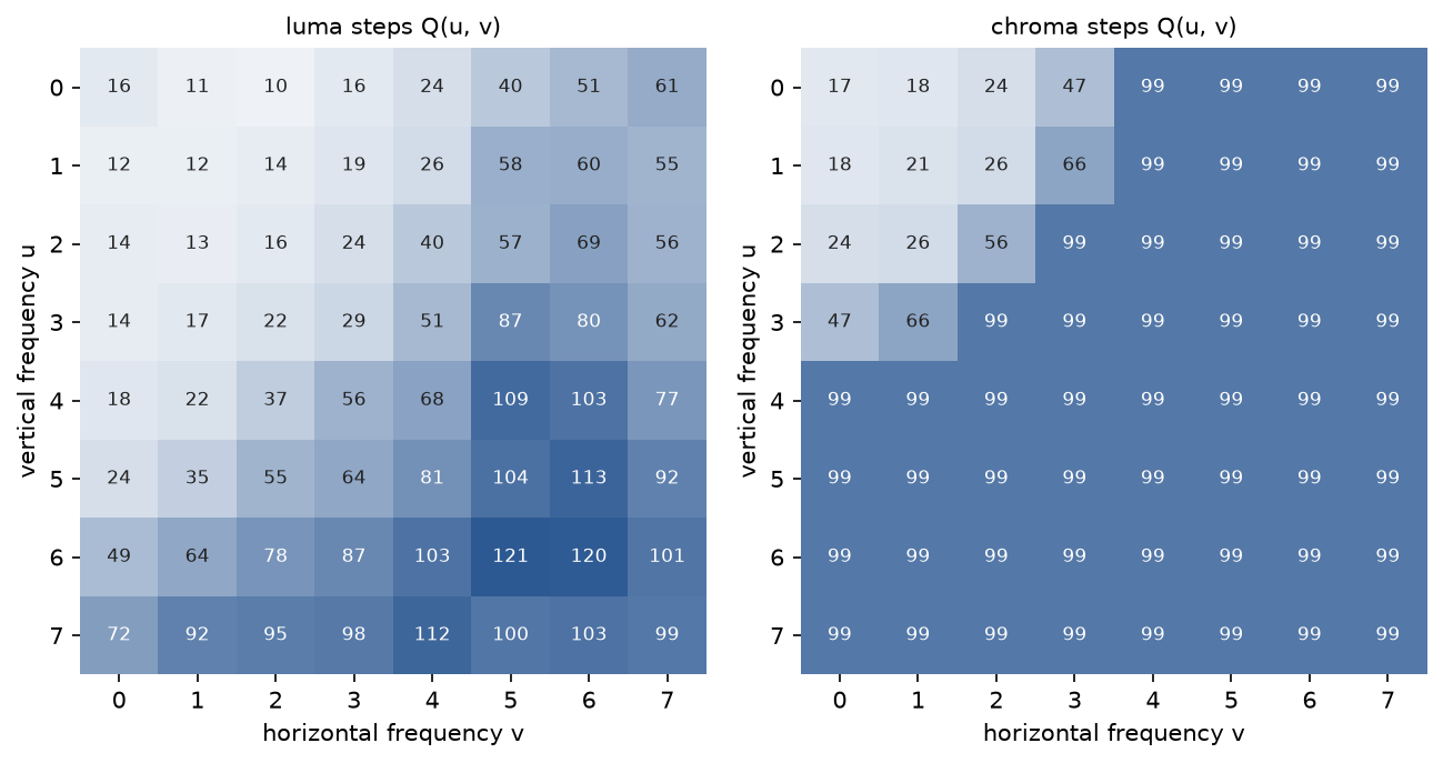
The luma table rises from 16, 11 and 10 in its first row to values above 100 in the bottom right, while the chroma table jumps to 99 almost everywhere outside its top left 4x4 corner, so most colour detail beyond the lowest frequencies is discarded.

A quality setting q is not part of the standard. The convention of the Independent JPEG Group's libjpeg, which Pillow and most tools follow, scales both tables by a percentage s(q), rounds, and clips the steps to the range of one byte:

Quality 50 gives the tables themselves, quality 10 multiplies them by 5 (clipped at 255), quality 90 by 0.2, and quality 100 sets every step to 1.

Zigzag order

The zigzag scan visits the coefficients by anti-diagonals u + v = 0, 1, ..., 14, alternating direction, so the sequence starts at (0, 0), (0, 1), (1, 0), (2, 0), (1, 1), (0, 2), (0, 3) and ends at (7, 7). In row-major indices the order begins 0, 1, 8, 16, 9, 2, 3, 10, 17, 24.

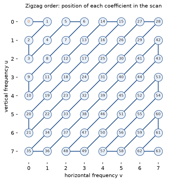
Low frequencies, which survive quantization, come first; high frequencies, mostly zero, form a long tail that a single end-of-block symbol can cover.

Entropy coding

The DC coefficients of neighbouring blocks are similar, so each block codes the difference from the previous block of the same component, with the predictor starting at 0 at the beginning of the scan:

Every integer x is described by its magnitude category m(x), the number of bits of its absolute value, followed by m(x) extra bits that pick one value of the category:

Category 0 holds only 0, category 1 holds -1 and 1, category 2 holds -3, -2, 2 and 3, category 3 holds -7 to -4 and 4 to 7, and so on. The extra bits of a negative value are the ones' complement of its magnitude, so the first extra bit is 1 for positive and 0 for negative values. The category of d is Huffman coded with the DC table, and is at most 11 for 8-bit images.

The 63 AC coefficients are coded as events. Each nonzero coefficient becomes one byte s that packs the run of zeros before it and its category, written (r, m), followed by m extra bits:

A run of more than 15 zeros uses ZRL = (15, 0), which stands for exactly 16 zeros and is only sent when a nonzero coefficient follows. After the last nonzero coefficient the end-of-block symbol EOB = (0, 0) closes the block, and it is omitted when z63 itself is nonzero.

The diagram shows both paths. The DC categories and the AC bytes are Huffman coded with separate tables for luma and chroma. A JPEG file describes each table by BITS, the number of codes of each length from 1 to 16, and HUFFVAL, the symbols in order of increasing code length. The codes are canonical: the first code is 0, each next code of the same length is one larger, and the code is doubled whenever the length grows. Two rules apply: no code is longer than 16 bits, and no code consists of ones only, so that the 1-bits used to pad the last byte never form a complete code.

The JPEG standard lists typical tables, used by default by most encoders. Optimal tables for one image come from its own symbol counts: run the Huffman algorithm with one extra symbol of count 1 that claims the all-ones code, shorten any code longer than 16 bits with the adjustment procedure of the standard's Annex K, and drop the extra symbol. With the code lengths of the DC and AC tables in use, the entropy-coded part of the image costs exactly

bits. The coded bits are then padded with 1-bits to a whole byte, and a zero byte is inserted after every 0xFF byte (byte stuffing) so that the decoder cannot mistake data for a marker.

The file

A baseline JFIF file is a sequence of segments, each introduced by a two-byte marker, around the entropy-coded data.

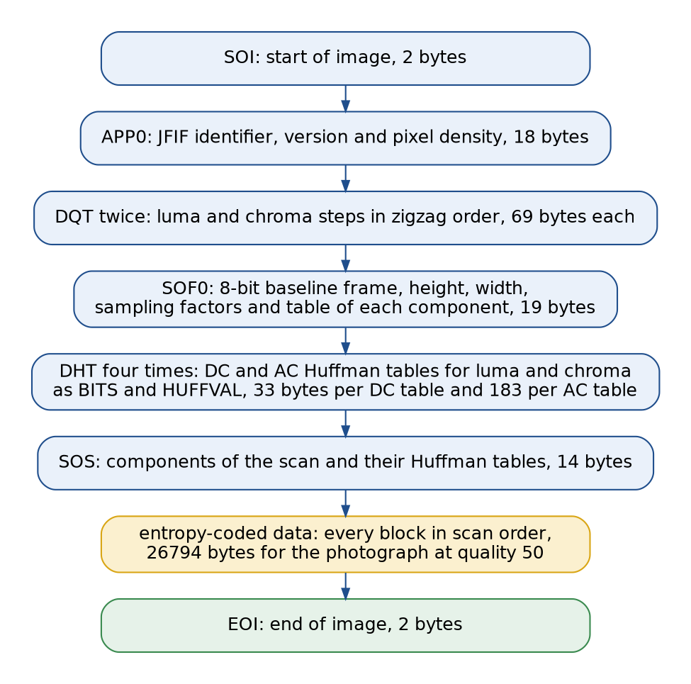
With the standard tables and 4:2:0 subsampling the headers take 625 bytes, so they matter only for tiny images. The scan visits the macroblocks in raster order, and each macroblock contributes its four luma blocks, then one Cb and one Cr block, as in the macroblock diagram above.

Measuring rate and quality

The rate is the size of the complete file, headers included, in bits per pixel:

The peak signal-to-noise ratio compares the decoded image y with the original x over all H W pixels and the three channels:

PSNR treats every error alike. The structural similarity index (SSIM) instead compares local means μ, variances σ² and the covariance σxy in a sliding window:

The local values are averaged over the image. Here the window is a Gaussian with standard deviation 1.5 truncated to 11x11, as in the original definition, and SSIM is computed on luma; 1 means identical. A simple blockiness index, the mean absolute luma step across block boundaries divided by the mean step inside blocks, is close to 1 for natural images and grows with visible blocking.

Worked example

Four pixels through the colour transform and 4:2:0

A 2x2 group straddles an edge between orange and blue, with the left column orange and the right column blue:

• Top left, RGB (212, 140, 64): Y = 152.8640, Cb = 77.8510, Cr = 170.1797.
• Top right, RGB (86, 118, 196): Y = 117.3240, Cb = 172.3995, Cr = 105.6576.
• Bottom left, RGB (206, 134, 58): Y = 146.8640, Cb = 77.8510, Cr = 170.1797.
• Bottom right, RGB (92, 124, 202): Y = 123.3240, Cb = 172.3995, Cr = 105.6576.

For the top-left pixel, Y = 0.299 × 212 + 0.587 × 140 + 0.114 × 64 = 63.388 + 82.18 + 7.296 = 152.864, Cb = (64 - 152.864) / 1.772 + 128 = 77.8510 and Cr = (212 - 152.864) / 1.402 + 128 = 170.1797. The bottom-left pixel is the top-left one minus 6 in every component, a grey offset, so its chroma is identical and only its luma drops by 6.

4:2:0 keeps one chroma pair for the group, the averages Cb = 125.1253 and Cr = 137.9187. Rebuilding the top-left pixel from its own luma and the shared chroma gives R = 152.864 + 1.402 × 9.9187 = 166.7700, and the pixel becomes (166.7700, 146.7700, 147.7700): a pinkish grey instead of orange, while its luma is still exactly 152.864. The top-right pixel becomes (131.2300, 111.2300, 112.2300). At a sharp colour edge subsampling destroys the colour of both sides; in smooth regions the four chroma values are nearly equal and averaging costs almost nothing.

One 8x8 block through the encoder

A patch of luma whose brightness rises from left to right, dips slightly in the middle rows and carries a fine vertical weave is coded at quality 50, so the step sizes are the luma table itself, and the previous block of the scan had a quantized DC coefficient of 7. Its rows are:

• Row 0: 109, 111, 129, 119, 146, 138, 156, 159.
• Row 1: 106, 108, 126, 120, 141, 135, 153, 156.
• Row 2: 105, 106, 124, 117, 141, 133, 155, 156.
• Row 3: 101, 104, 125, 118, 142, 135, 157, 153.
• Row 4: 107, 112, 129, 122, 143, 134, 156, 157.
• Row 5: 110, 112, 132, 124, 148, 141, 160, 161.
• Row 6: 119, 121, 139, 130, 156, 147, 168, 166.
• Row 7: 128, 127, 144, 139, 163, 156, 172, 174.

Level shift. Subtracting 128 gives f, whose first row is -19, -17, 1, -9, 18, 10, 28, 31. Its energy, the sum of the squared samples, is 28259.

DCT. For the first row of coefficients, u = 0, the vertical cosine is constant, so only the column sums S of f matter. They are -139, -123, 24, -35, 156, 95, 253 and 258, and the first row of coefficients is

The DC coefficient is one eighth of the sum of all samples, eight times the block mean of 135.640625 minus 128:

For v = 1 the cosines of columns j and 7 - j are opposite, so the column sums pair up as S0 - S7 = -397, S1 - S6 = -376, S2 - S5 = -71 and S3 - S4 = -191, to be multiplied by the cosines 0.9808, 0.8315, 0.5556 and 0.1951:

The cosines were rounded to four decimals there; at full precision F(0, 1) = -137.6581. All 64 coefficients, row u by row:

• u = 0: 61.1250, -137.6581, 0.4175, -14.3171, -1.1250, -4.3219, -1.9318, 45.9158.
• u = 1: -44.2961, -1.6156, 1.3980, -1.7493, -0.1832, -0.6003, 0.4481, -0.1604.
• u = 2: 33.0459, 2.6019, 1.3384, 3.1234, 1.9879, -2.3436, 2.3044, -0.6077.
• u = 3: -5.2090, 1.4340, 0.1005, -1.7015, -1.0834, -1.7053, 0.3839, 0.7226.
• u = 4: 6.1250, 0.3346, -1.0476, 0.3496, -0.1250, -0.4300, -0.2426, -0.1355.
• u = 5: -1.2789, -2.8868, -0.7383, 1.9034, -2.0876, 0.2747, -0.6163, 3.2018.
• u = 6: 1.0595, -1.5773, 1.0544, 0.8485, 1.2061, -0.6732, 1.1616, 0.2764.
• u = 7: 2.0674, 2.9484, 2.7306, -1.1675, 0.6099, -1.0851, -1.5593, 0.5424.

The sum of their squares is again 28259. The horizontal ramp shows up in F(0, 1), which alone holds 67.06 % of the energy; the dip in the middle rows in F(2, 0); and the weave, a pattern that alternates from column to column, in F(0, 7). The first six coefficients in zigzag order hold 91.10 % of the energy.

Quantization. Dividing by the luma steps and rounding leaves six nonzero coefficients:

• (0, 0): 61.1250 / 16 = 3.8203, rounded to 4.
• (0, 1): -137.6581 / 11 = -12.5144, rounded to -13.
• (1, 0): -44.2961 / 12 = -3.6913, rounded to -4.
• (2, 0): 33.0459 / 14 = 2.3604, rounded to 2.
• (0, 3): -14.3171 / 16 = -0.8948, rounded to -1.
• (0, 7): 45.9158 / 61 = 0.7527, rounded to 1.

Every other ratio is below 0.5 in magnitude and rounds to zero; the largest of them is (3, 0) with -5.2090 / 14 = -0.3721. The ratio for F(0, 1) lies only 0.0144 beyond the rounding boundary at -12.5. Six of 64 coefficients survive, and they hold 99.27 % of the energy.

Zigzag. Positions 0 to 3 are (0, 0), (0, 1), (1, 0) and (2, 0); position 6 is (0, 3) and position 28 is (0, 7). The sequence is therefore 4, -13, -4, 2, 0, 0, -1, then 21 zeros, then 1 at position 28, then 35 zeros.

Symbols and bits, with the standard luma Huffman tables:

• DC: d = 4 - 7 = -3, category 2, code 011, extra bits 00, 5 bits.
• Position 1: (0, 4) for -13, code 1011, extra bits 0010, 8 bits.
• Position 2: (0, 3) for -4, code 100, extra bits 011, 6 bits.
• Position 3: (0, 2) for 2, code 01, extra bits 10, 4 bits.
• Positions 4 to 6: (2, 1) for -1 after two zeros, code 11100, extra bit 0, 6 bits.
• Positions 7 to 22: ZRL for sixteen zeros, code 11111111001, 11 bits.
• Positions 23 to 28: (5, 1) for 1 after the remaining five zeros, code 1111010, extra bit 1, 8 bits.
• Positions 29 to 63: EOB, code 1010, 4 bits.

The negative values use the ones' complement rule: -3 in category 2 is -3 + 3 = 0, written 00; -13 in category 4 is -13 + 15 = 2, written 0010; -4 in category 3 is -4 + 7 = 3, written 011. The run of 21 zeros before position 28 does not fit in four bits, so a ZRL takes 16 of them and the symbol (5, 1) the remaining five. The block becomes the 52-bit string

0110010110010100011011011100011111111001111101011010

against 64 × 8 = 512 bits raw: 0.8125 bits per pixel, 9.85 times smaller. As the first block of a scan, with predictor 0, the DC difference would be 4, category 3, and the block would cost 53 bits.

The same block through the decoder

Dequantization multiplies back: row 0 becomes 64, -143, 0, -16, 0, 0, 0, 61, column 0 becomes 64, -48, 28 and then zeros, and everything else stays zero. The inverse DCT gives values such as -20.7906 and -22.2072 at the start of the first row. Adding 128 and rounding gives the reconstruction:

• Row 0: 107, 106, 130, 118, 146, 135, 159, 157.
• Row 1: 106, 104, 129, 117, 145, 133, 157, 156.
• Row 2: 104, 103, 127, 115, 143, 132, 156, 154.
• Row 3: 105, 103, 127, 116, 144, 132, 156, 155.
• Row 4: 108, 107, 131, 119, 147, 135, 160, 158.
• Row 5: 114, 112, 137, 125, 153, 141, 165, 164.
• Row 6: 120, 118, 143, 131, 159, 147, 171, 170.
• Row 7: 124, 122, 147, 135, 163, 151, 175, 174.

The error against the original starts -2, -5, 1, -1, 0, -3, 3, -2 in row 0, and no error anywhere exceeds 5 grey levels. The mean squared error of the coefficients, the average of the 64 squared differences between F and F̃, is 7.9983 and equals that of the samples before rounding, as Parseval predicts; rounding to integers raises it to 534 / 64 = 8.34375, a PSNR of 10 log10(255² / 8.34375) = 38.9172 dB. The weave survives as a single coefficient.

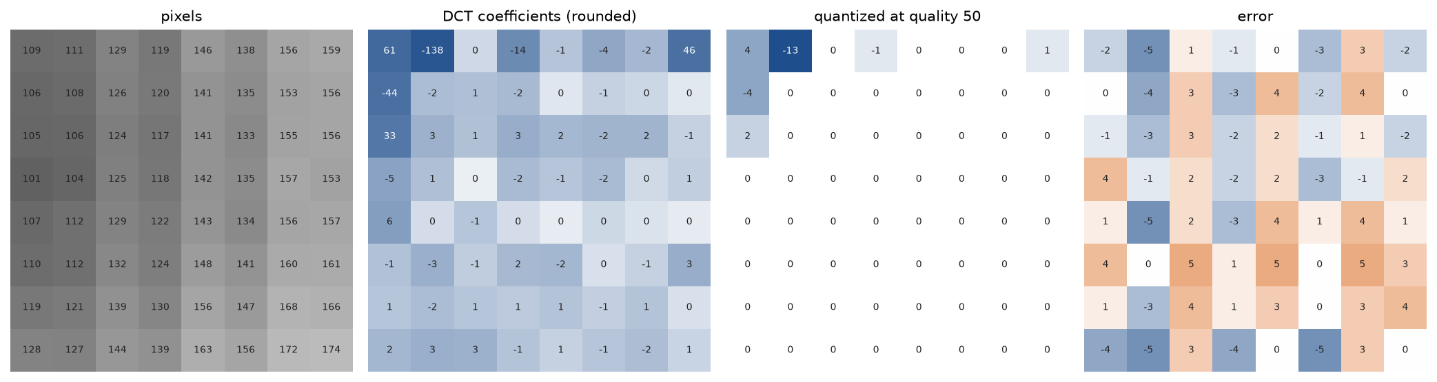
The panels show the whole journey at a glance: 64 pixels, a handful of large coefficients in the first row and column, six survivors, and an error with no visible structure. Every number in this section is asserted by tests/test_trace.py and printed by examples/worked_block.py.

The code

The package jpeg_from_scratch needs only NumPy for the codec itself. Pillow is imported inside the functions that load the photograph and run Pillow's codec, SciPy inside the DCT comparison, and Matplotlib only by the plotting modules. One idea lives in each module:

• arrays.py holds the array types, the block size, the level shift and to_uint8, the final rounding.
• colour.py builds the RGB to YCbCr matrix from the two luma weights, with rgb_to_ycbcr, ycbcr_to_rgb and luma.
• planes.py pads planes to whole macroblocks, subsamples and upsamples chroma, splits planes into 8x8 blocks and merges them back, and measures subsampling alone with chroma_round_trip.
• transform.py holds the DCT matrix, the definition with four loops (dct2_direct, idct2_direct) and the matrix form (dct2, idct2), which transforms any number of blocks at once.
• compaction.py measures energy compaction: the ramp under the DCT and the DFT, and the KLT, DCT and pixel curves of a real image.
• quantization.py holds the two standard tables, libjpeg's quality scaling and the quantizer, which rounds half away from zero.
• zigzag.py builds the zigzag order and converts blocks to and from it.
• symbols.py turns a zigzag sequence into DC and AC symbols with their extra bits, and back.
• huffman.py holds HuffmanTable as BITS and HUFFVAL with its canonical codes, the four standard tables, and the length-limited construction of optimal tables.
• scan.py orders the blocks of the scan, keeps one DC predictor per component, counts the coded bits exactly and produces the stuffed bytes.
• jfif.py writes the marker segments and parses any baseline file, including Pillow's.
• encoder.py holds encode, which returns an EncodedImage with the coefficients, tables, exact bit count and file bytes, and decoder.py holds decode, which reads a file back through Huffman decoding, dequantization, the inverse DCT and upsampling.
• metrics.py holds bits per pixel, MSE, PSNR, SSIM and the blockiness index.
• analysis.py splits an encoded image's bits by kind of symbol and computes the cost of every macroblock.
• trace.py holds the worked examples: trace_colour_group, trace_block, which keeps every stage of one block, first_row_by_hand and format_block_trace.
• datasets.py generates the synthetic scene and downloads and verifies the photograph.
• comparisons.py runs Pillow's encoder and decoder and SciPy's DCT, and measures rate and quality curves for either codec.
• pitfalls.py holds deliberately wrong versions of single steps for the Pitfalls section.
• plotting.py and image_plots.py draw every figure in the handbook's four colours.

The heart of the encoder is a few lines per component; the same loop serves greyscale, 4:4:4 and 4:2:0:

for index, (plane, (h, v)) in enumerate(zip(planes, sampling)):
    padded = pad_plane(plane, mcu_rows * BLOCK * v_max, mcu_cols * BLOCK * h_max, padding)
    reduced = downsample(padded, v_max // v, h_max // h)
    blocks = split_blocks(reduced - LEVEL_SHIFT)
    coefficients.append(quantize(dct2(blocks), tables[0 if index == 0 else 1]))

and the AC run-length coder walks only over the nonzero coefficients:

for position in np.flatnonzero(values[1:]) + 1:
    run = int(position) - previous - 1
    while run > 15:
        symbols.append(ZERO_RUN)
        run -= 16
    value = int(values[position])
    category = magnitude_category(value)
    symbols.append(Symbol("ac", run, category, value))
    previous = int(position)
if previous != BLOCK * BLOCK - 1:
    symbols.append(END_OF_BLOCK)

The examples and the project import the package, so install the repository first as described in the main README. The examples each demonstrate one idea and run in a few seconds from the repository root:

• examples/worked_block.py prints every stage of the worked block, the first row of coefficients by hand and the bit string, and saves the worked-block, quantization-table and zigzag figures.
• examples/chroma_subsampling.py prints the colour matrix, the four-pixel example, the cost of subsampling alone on both images and the trade between 4:2:0 and 4:4:4 at quality 90, and saves the YCbCr planes.
• examples/energy_compaction.py checks the DCT three ways, compares the DCT with the DFT on the ramp and with the KLT on the photograph, and saves the basis images and the compaction curves.
• examples/bit_budget.py encodes the photograph at quality 50, splits its bits by kind of symbol, builds optimized Huffman tables, lists the segments of the file and saves the cost of every macroblock.
• examples/artefacts.py measures blockiness across quality settings and saves crops of the three artefacts and a luma profile across a thin edge.
• examples/common_mistakes.py measures every mistake listed under Pitfalls.

python signal-processing/jpeg-from-scratch/examples/worked_block.py
python signal-processing/jpeg-from-scratch/examples/chroma_subsampling.py
python signal-processing/jpeg-from-scratch/examples/energy_compaction.py
python signal-processing/jpeg-from-scratch/examples/bit_budget.py
python signal-processing/jpeg-from-scratch/examples/artefacts.py
python signal-processing/jpeg-from-scratch/examples/common_mistakes.py

The sample project, project/jpeg_encoder.py, is a command-line JPEG encoder. It takes image files, or the names photograph and scene for the two bundled test images, encodes each at the chosen quality and subsampling into a real baseline JFIF file in .data/jpeg-from-scratch/encoded/, checks that Pillow opens the file, decodes it back with our own decoder, and reports the size, rate, PSNR, SSIM and blockiness next to Pillow's encoder at the same settings. It then confirms that Pillow's quantization tables equal ours at all 100 quality settings, sweeps twelve quality settings for both codecs and saves the rate and quality curves. Options --quality, --subsampling, --optimize, --output and --sweep change the run, and --figures sends the PNG to another folder so a custom run does not overwrite the one shown here; the default run takes a few seconds.

python signal-processing/jpeg-from-scratch/project/jpeg_encoder.py
python signal-processing/jpeg-from-scratch/project/jpeg_encoder.py scene --quality 80 --subsampling 4:4:4 --optimize --figures custom-figures

With the defaults the photograph becomes a file of 27419 bytes, 625 of them headers: 0.9140 bits per pixel, 30.51 dB and SSIM 0.9123, against 27355 bytes, 0.9118 bits per pixel, 30.50 dB and 0.9124 from Pillow, and Pillow's decoding of our file agrees with ours to 53.80 dB. The scene becomes 10026 bytes against Pillow's 9868, at 29.99 against 29.97 dB.

The notebook jpeg_from_scratch.ipynb follows this page: the worked block through trace_block and again in bare NumPy, the colour example and the cost of subsampling, the DCT three ways with its basis images, energy compaction against the DFT and the KLT, the quantization tables, the symbol statistics and bit budget of a whole image, the finished file, a demonstration of each pitfall below, the rate and quality of both test images with their artefacts, and the comparison with Pillow. The tests in tests check the worked examples value by value, the properties above and the agreement with Pillow and SciPy, and run in a few seconds:

python -m pytest signal-processing/jpeg-from-scratch

Data: the synthetic scene is generated by synthetic_scene from a seed, so nothing is downloaded for it. The photograph is the coffee-cup image distributed with scikit-image, released under CC0 by its photographer, Rachel Michetti, courtesy of Pikolo Espresso Bar. download_photograph fetches it from the scikit-image repository at tag v0.24.0 (skimage/data/coffee.png) into .data/jpeg-from-scratch/ at the repository root and verifies its SHA-256 digest.

In practice

SciPy's scipy.fft.dctn(block, type=2, norm="ortho") agrees with dct2 to about 10⁻¹³, and so does the definition with four loops. Pillow wraps libjpeg (libjpeg-turbo in current wheels), and comparing our encoder with Image.save(buffer, "JPEG", quality=q, subsampling=2) checks every stage at once:

• Its quantization tables equal ours at all 100 quality settings, and its Huffman tables are the standard ones (test_quality_scaling_matches_pillow and test_standard_huffman_tables_match_pillow in tests/test_comparisons.py).
• Pillow opens the files our encoder writes, and our decoder opens Pillow's. On the photograph at quality 50 the two decoders agree to a PSNR of 53.8 dB on either file, and on Pillow's file no pixel differs by more than 3 grey levels, far below the coding error. The differences come from libjpeg's integer DCT, its fixed-point colour conversion and the rounding in its resampling.
• At quality 50 the entropy-coded data of the photograph takes 26794 bytes from our encoder and 26730 from Pillow's, and 26081 against 26002 with optimized Huffman tables (optimize=True in Pillow).

Rate and quality of both images with 4:2:0 and the standard Huffman tables, the rate including the 625 bytes of headers, ours first and Pillow's second:

• Photograph at quality 10: 0.3241 and 0.3227 bits per pixel, 26.04 and 26.03 dB, SSIM 0.7653 for both.
• Photograph at quality 20: 0.5072 and 0.5050 bits per pixel, 28.06 and 28.05 dB, SSIM 0.8453 for both.
• Photograph at quality 50: 0.9140 and 0.9118 bits per pixel, 30.51 and 30.50 dB, SSIM 0.9123 and 0.9124.
• Photograph at quality 80: 1.6024 and 1.6000 bits per pixel, 33.21 and 33.19 dB, SSIM 0.9537 and 0.9536.
• Photograph at quality 95: 3.4721 and 3.4904 bits per pixel, 37.53 and 37.46 dB, SSIM 0.9878 and 0.9875.
• Scene at quality 10: 0.3912 and 0.3887 bits per pixel, 25.65 and 25.64 dB, SSIM 0.8841 and 0.8839.
• Scene at quality 50: 0.8556 and 0.8421 bits per pixel, 29.99 and 29.97 dB, SSIM 0.9689 for both.
• Scene at quality 95: 2.3916 and 2.4022 bits per pixel, 33.27 and 33.25 dB, SSIM 0.9967 and 0.9969.

Over all twelve quality settings from 5 to 95 our files are between 0.5 % smaller and 1.9 % larger than Pillow's, and the PSNR differs by at most 0.07 dB (test_rate_and_quality_track_pillow checks three settings on the scene).

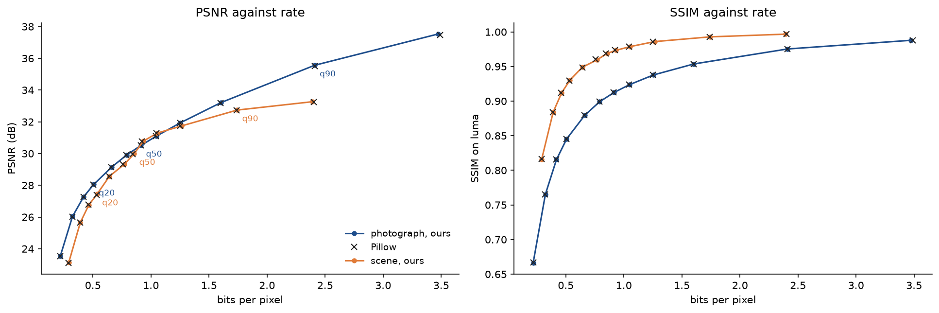
The crosses sit on the lines across the whole range, so the two encoders make the same trade between rate and quality. What the curves and the examples show:

• Quality settings are table multipliers, not quality levels. At quality 50 the scene costs 0.86 bits per pixel and reaches 29.99 dB; the photograph costs 0.91 and reaches 30.51 dB. On the photograph, going from about 0.5 to about 1 bit per pixel buys 3 dB.
• Subsampling caps the scene. Its saturated colour edges lose so much in 4:2:0 alone that, with no quantization at all, PSNR stops at 33.73 dB with linear upsampling (39.90 dB for the photograph). At quality 90, 4:4:4 lifts the scene from 32.74 to 39.75 dB for 30 % more bits; the photograph gains 1.7 dB for 29 % more bits, and its SSIM on luma barely changes (0.9753 against 0.9754), because subsampling affects only chroma.
• The bits go to texture and edges. In the photograph at quality 50 the brightly lit wood grain, the rim and the spoon cost several times more per pixel than the saucer, the shadow and the crema, and the costliest 20 % of macroblocks hold 37 % of the bits. Over the whole file, Huffman codes of AC symbols take 53 % of the bits, their extra bits 25 %, end-of-block codes 9 % and DC 13 %; 21 % of all blocks have no nonzero AC coefficient at all.
• Optimized Huffman tables save 2.5 % on the photograph at quality 50, for example by shortening the luma end-of-block code from 4 to 3 bits and the zero run from 11 to 9; they cost a second pass over the data, which is why encoders make them optional.

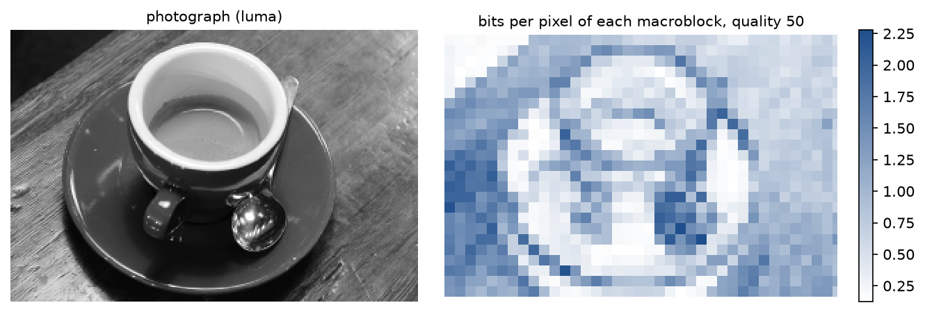
The map is the image's texture seen through the coder: flat regions cost a DC difference and an end-of-block code per block, while every edge and grain line adds AC symbols.

At low quality the artefacts are easy to name. In the crops below at quality 10, the sky turns into flat 8x8 tiles, the stripes and the rim ring, and the red patch acquires blurred, overshooting colour fringes. The blockiness index rises from 0.99 for both originals to 1.35 (photograph) and 1.14 (scene) at quality 50 and to 2.60 and 1.68 at quality 10.

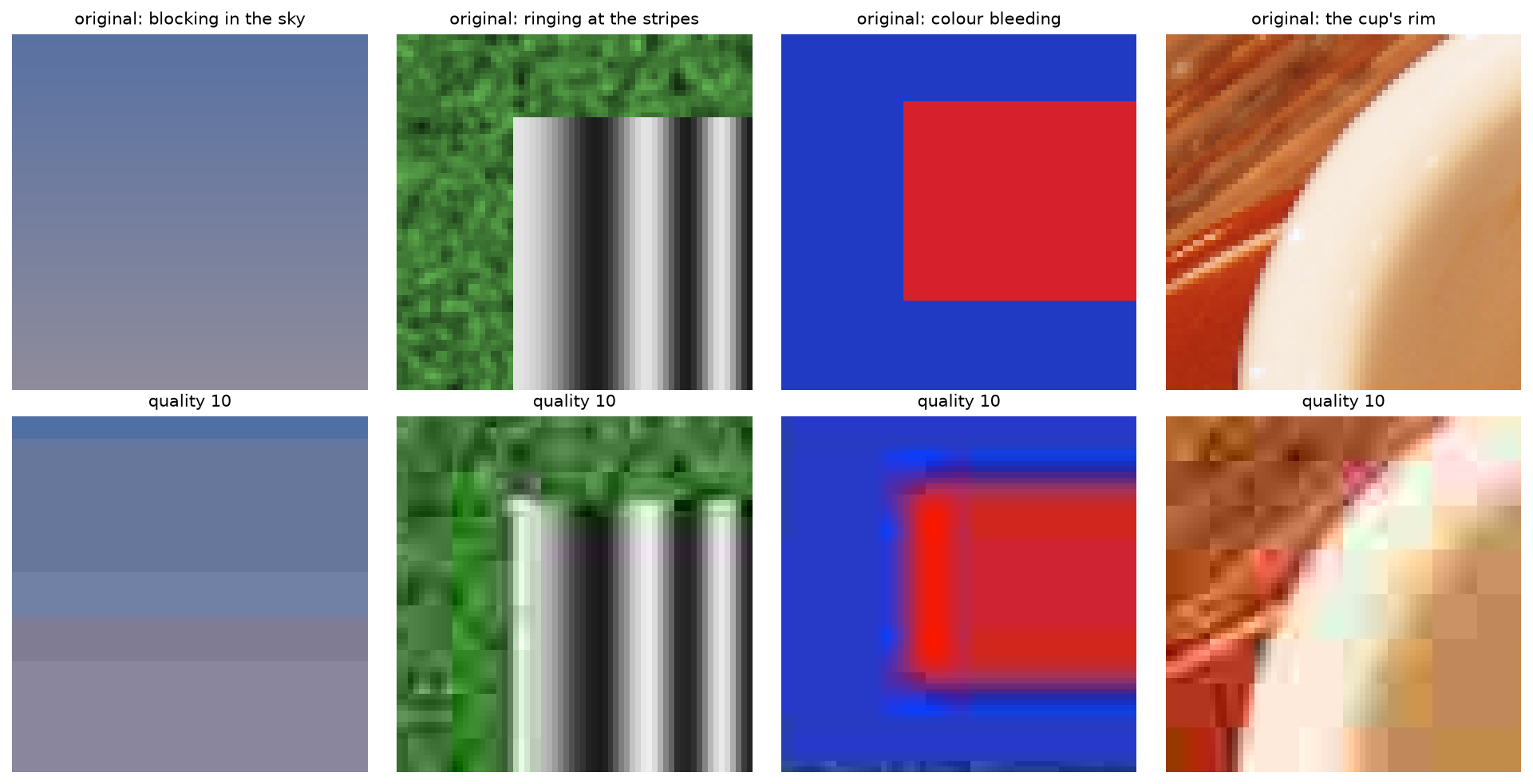
Each column isolates one artefact: blocking where a smooth gradient keeps only its block averages, ringing where sharp stripes lose their high frequencies, and colour bleeding where 4:2:0 and coarse chroma steps smear a saturated edge.

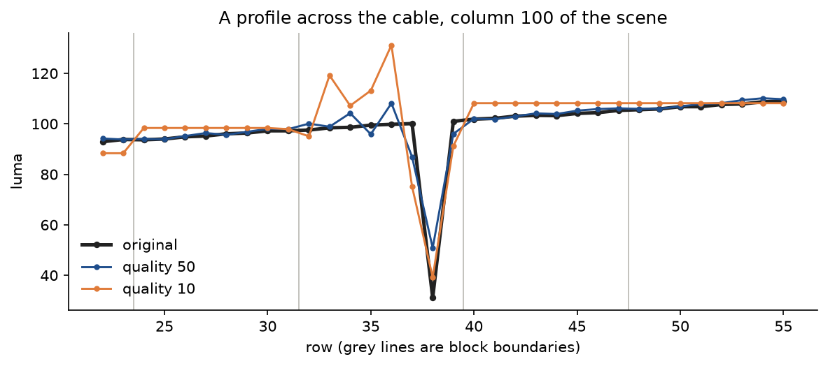
The profile shows both artefacts in one dimension. At quality 10 the block that contains the cable oscillates around it (ringing), while the blocks above and below are flat and meet with a step at their boundary (blocking); at quality 50 the oscillation is smaller and the sky follows its gradient again. In both, the dip of the cable comes back shallower than the original 31, at 51 for quality 50 and 39 for quality 10.

When to use which:

• Use Pillow, or libjpeg-turbo directly, for real work: it is fast (SIMD, integer arithmetic), robust and supports progressive and other modes this page leaves out. Pass subsampling=0 when colour edges matter, for example in screenshots or graphics, and optimize=True when a few per cent of size matter more than encoding time.
• Use the from-scratch version to learn the format, to experiment with tables, quantizers or block sizes, and to compute exact bit counts and per-block statistics that libraries do not expose.
• For better rate at the same quality, encoders such as mozjpeg keep the JPEG format but choose coefficients more cleverly, and newer formats (WebP, AVIF, JPEG XL) replace it. Learned image codecs go further still at a much higher computational cost.
• JPEG artefacts are a frequent, silent difference between training and deployment images for vision models; Training image classifiers treats such dataset shift. Video coding builds on the same transform and quantization ideas.

Pitfalls

Every number below is printed by examples/common_mistakes.py, and the notebook has a section for each mistake.

• Inverted compression ratios. A compression ratio is the original size divided by the compressed size, and a value below 1 is an expansion. Run-length coding that writes each byte as a (value, count) pair turns the 720000 raw bytes of the photograph into 1434968 bytes, a ratio of 0.5018. Dividing the other way round reports 1.99 for a file that doubled in size. Notebook section "A compression ratio below one".
• Calling every step lossy, or quality 100 lossless. Within JPEG only subsampling, quantization and rounding lose information: the colour transform returns the photograph to within 6 × 10⁻¹⁴ and the DCT its luma blocks to within 3 × 10⁻¹³. Conversely, quality 100 is not lossless. With 4:4:4 it reaches 50.62 dB at 11.91 bits per pixel; with 4:2:0 subsampling caps it at 39.71 dB. Notebook section "Which steps lose information".
• The wrong DCT normalization. The standard tables assume the orthonormal DCT. scipy.fft.dctn without norm="ortho" returns the 2-D coefficients 16 times larger in general, 16√2 times larger in the first row and column, and 32 times larger for DC, so the same tables quantize far too finely: the photograph's luma plane keeps 135297 nonzero coefficients instead of 33986, and its DC differences exceed the 11 bits baseline JPEG allows (test_unnormalized_scipy_dct_is_larger). Likewise the factor 1/4 in the usual formula is 2/N for N = 8, not a constant for every block size. Notebook section "DCT normalization".
• The transform written the wrong way round. Tᵀ f T is the inverse DCT. Paired with T F Tᵀ at the decoder it still returns the image exactly, so a round-trip test passes, but the coefficients no longer compact energy: on the photograph's luma at quality 50 it costs 338409 bits instead of 186757 (81 % more) and loses 2.08 dB. Test reconstruction after quantization, and compare with a reference such as scipy.fft.dctn. Notebook section "The transform the wrong way round".
• Quantization tables in natural order inside the file. DQT stores the 64 steps in zigzag order. A writer that stores them row by row produces a file that every decoder accepts and dequantizes with the wrong steps: the photograph drops from 30.51 to 22.58 dB, in our decoder and in Pillow alike. Current Pillow versions return the quantization attribute in natural order, so tables read from Pillow must be reordered before they are written. Notebook section "Quantization tables in the wrong order".
• Zero padding at the right and bottom edges. Filling the padding with zeros places a black edge inside the last blocks. On the scene, 375 pixels wide, at quality 75 it costs 7.7 % more bytes and drops the PSNR of the last 7 columns from 33.56 to 19.88 dB, because the ringing of the artificial edge spills into visible pixels. Repeat the edge pixels. Notebook section "Zero padding at the right and bottom edges".
• Unsigned arithmetic in PSNR. uint8 subtraction wraps around: np.array([10], np.uint8) - np.array([20], np.uint8) is 246, and squaring then overflows as well. Computed this way the photograph at quality 50 reports 33.14 dB instead of 30.51 dB. Convert to float before subtracting, as mse does (test_mse_and_psnr_use_signed_arithmetic). Notebook section "Unsigned arithmetic in PSNR".
• ZRL for trailing zeros, EOB after a final nonzero. ZRL is only for runs followed by a nonzero coefficient; the EOB covers trailing zeros, and it must be omitted when z63 is nonzero. Emitting a ZRL for every 16 zeros up to the end of each block is still decodable but costs 73 % more bits on the photograph (test_zero_runs_and_end_of_block checks the correct rules). Notebook section "Zero runs at the end of a block".
• One DC predictor for all components. Each component keeps its own DC predictor, reset to 0 at the start of the scan. Carrying one predictor across the Y, Cb and Cr blocks costs 7.0 % more bits on the photograph, and standard decoders read the result as noise: 9.43 dB with ours and 5.60 dB with Pillow. Notebook section "One DC predictor for all components".
• Comparing decoders that upsample differently. The same file decoded with nearest upsampling gives 30.29 dB, with linear upsampling 30.51 dB, and with Pillow's decoder 30.50 dB. Codec comparisons must decode with the same upsampling, or measure PSNR on luma only. Notebook section "Comparing decoders with different upsampling".
• Reading the quality setting as a measure of quality. The quality number only scales the tables. Quality 50 gives the scene 29.99 dB at 0.86 bits per pixel and the photograph 30.51 dB at 0.91, and above quality 90 the scene's PSNR hardly moves (32.74 dB at 90, 33.27 dB at 95) because subsampling limits it. Other encoders map the same number to different tables, and some use different base tables altogether, so compare codecs by measured rate and distortion, as in the figure above, never by their quality settings. Notebook section "A realistic run".

Further reading

• ITU-T Recommendation T.81 and ISO/IEC 10918-1, Information technology: Digital compression and coding of continuous-tone still images, requirements and guidelines, 1992. The JPEG standard; Annex K holds the example tables and the length-limited Huffman procedure.
• G. K. Wallace, "The JPEG still picture compression standard", Communications of the ACM 34(4), 30-44, 1991. The classic overview of the baseline system.
• W. B. Pennebaker and J. L. Mitchell, JPEG Still Image Data Compression Standard, Van Nostrand Reinhold, 1993.
• E. Hamilton, JPEG File Interchange Format, version 1.02, C-Cube Microsystems, 1992. The JFIF colour equations and file layout.
• N. Ahmed, T. Natarajan and K. R. Rao, "Discrete cosine transform", IEEE Transactions on Computers C-23(1), 90-93, 1974. Introduces the DCT and compares it with the Karhunen-Loeve transform.
• K. R. Rao and P. Yip, Discrete Cosine Transform: Algorithms, Advantages, Applications, Academic Press, 1990.
• Y. Arai, T. Agui and M. Nakajima, "A fast DCT-SQ scheme for images", Transactions of the IEICE E71(11), 1095-1097, 1988. The fast 8-point DCT used by many JPEG codecs.
• D. A. Huffman, "A method for the construction of minimum-redundancy codes", Proceedings of the IRE 40(9), 1098-1101, 1952.
• Z. Wang, A. C. Bovik, H. R. Sheikh and E. P. Simoncelli, "Image quality assessment: from error visibility to structural similarity", IEEE Transactions on Image Processing 13(4), 600-612, 2004.
• K. Sayood, Introduction to Data Compression, fifth edition, Morgan Kaufmann, 2017. Transform coding, quantization and rate-distortion in depth.
• J. Balle, V. Laparra and E. P. Simoncelli, "End-to-end optimized image compression", International Conference on Learning Representations, 2017. A learned successor to the transform-quantize-code pipeline.