Optimizers

Backpropagation delivers the gradient of the cost with respect to every weight; the optimizer decides what to do with it. Plain gradient descent takes a step of fixed size against the gradient, which is slow when the cost surface is a long narrow valley, erratic when the gradient is estimated from a small batch, and hopeless when one bad step lands on a cliff. The optimizers used in practice answer each problem with a small amount of memory: momentum keeps a running sum of past gradients, AdaGrad, RMSProp and Adam keep a running size of each coordinate's gradient and divide by it, AdamW takes weight decay out of that division, a schedule changes the learning rate over time, and clipping caps the length of any single step. This page derives each update from first principles, including the convergence rate of momentum on an ill-conditioned quadratic and the bias correction of Adam, works three steps of every method by hand, draws all of them on the same contour plots of a quadratic, the Rosenbrock valley and a saddle point, and benchmarks every optimizer and schedule on one small network after tuning each learning rate. Everything is implemented from scratch in NumPy and checked step for step against torch.optim and torch.optim.lr_scheduler. Afterwards you will be able to carry out any of these updates on paper, predict how momentum and adaptive scaling change the path through a cost surface, choose a learning rate and schedule with evidence rather than habit, and read optimizer code in any framework.

To run the code in this topic, install the base group, and the deep group for the comparisons with PyTorch.

Intuition

Picture the cost as a landscape and the parameters as a ball. Gradient descent moves the ball a fixed fraction of the local slope at every step. In a long narrow valley the slope points mostly across the valley, so the ball bounces from wall to wall and creeps along the floor; a larger step makes the bouncing diverge. Three ideas change this.

• Give the ball inertia. If each step adds the new gradient to a decaying memory of the old ones, the components that keep pointing the same way, along the valley floor, accumulate, while the components that flip sign, across the valley, cancel. This is momentum, and on a quadratic it turns a slowdown proportional to the condition number κ into one proportional to √κ. Nesterov's variant looks at the slope where the momentum is about to carry the ball rather than where it stands.
• Give every coordinate its own step size. If each coordinate's step is divided by the typical size of its recent gradients, steep and flat directions move at similar speeds. AdaGrad divides by the root of the sum of all past squared gradients, RMSProp by a moving average, and Adam combines the moving average with momentum and corrects both averages for starting at zero. This works when the steep and flat directions line up with the coordinate axes; for a rotated valley it does not, a fact the contour plots below show directly.
• Change the step size over time. Early in training, large steps make fast progress; late in training, the noise of mini-batch gradients keeps a constant-step optimizer hopping around the minimum at a distance proportional to the step, and only a smaller step lets it settle. Schedules such as step decay, cosine annealing, warmup and the one-cycle policy encode this, and the learning-rate range test finds the largest step worth using in a single short run.

Two guards complete the picture. Weight decay shrinks every weight a little at each step, and AdamW applies it outside Adam's division so that it shrinks every weight equally. Gradient clipping rescales any gradient longer than a threshold, so that a single cliff in the landscape cannot throw the parameters away.

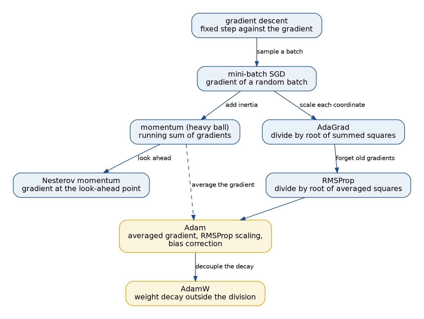
The diagram shows how the methods on this page build on one another. Each arrow adds one idea, named on the arrow; Adam is the meeting point of the two branches, an averaged gradient divided by an averaged square, and AdamW changes only how it applies weight decay.

The second diagram shows where each piece enters a training step. Clipping acts on the gradient before the optimizer sees it, the schedule only sets the learning rate (and, for one-cycle, the momentum) of the current step, and the optimizer's state, its running averages and step count, is the only thing an optimizer carries from one step to the next.

How it works

Notation

The network notation of Backpropagation carries over: W and b are the weights and biases of a layer, C is the cost, m the mini-batch size and η the learning rate. The formula images write the step as a subscript t; in the text, a quantity is named in words with the step it belongs to, for example "the velocity v after step t", and the start is θ₀. Adam's two decay rates are written β1 and β2, plainly, just as W1 stands for the weights of layer 1 in Backpropagation.

• θ holds all parameters, every W and b flattened into one column. The gradient g used at step t is computed at the parameters before that step, as the batch averages of equations B3 and B4.
• The cost is the average of N per-example costs, and the batch of each step is a set of m indices drawn at random.
• η is the learning rate; under a schedule it changes with the step.
• β is the momentum coefficient, v the velocity or first moment, a running sum or average of gradients, and s a running sum or average of squared gradients. Both start at zero.
• ρ is the decay rate of RMSProp's average, called alpha in PyTorch; β1 and β2 are Adam's decay rates for v and s, and v̂ and ŝ their bias-corrected values.
• ε is a small constant that keeps a denominator away from zero, and λ is the coefficient of an L2 penalty or of weight decay.
• H is the Hessian of the cost, with eigenvalues from λmin to λmax (the subscripts tell them apart from the decay λ), and κ = λmax / λmin is the condition number.
• Σ is the covariance of the per-example gradients, and its trace, tr Σ, the total gradient variance.

Products, squares, square roots and quotients of vectors act entry by entry: the square of g is the vector of squared entries, and g divided by the root of s divides each entry by the root of the matching entry.

Gradient descent, briefly

Gradient descent repeats one update:

Near a minimum θ* every smooth cost looks like a quadratic whose gradient is H times the distance to the minimum. Along an eigenvector of H with eigenvalue λi the error is multiplied by 1 - ηλi at every step, which gives the two facts below:

Calculus and optimization derives these facts. Two of them drive everything below: the cost of gradient descent grows linearly with κ, and the step size is capped by the steepest direction however flat the others are.

Stochastic and mini-batch gradients

A network's cost is an average over N examples, and the exact gradient costs a pass over all of them. A mini-batch of m indices drawn at random gives an estimate that is unbiased because every example is equally likely to be drawn:

The size of its error can be computed exactly. Let ui be the difference between example i's gradient and the full gradient; these differences sum to zero. For a batch drawn without replacement, as data loaders do within an epoch, let Ii indicate that example i is in the batch. The expected squared length of the sum of the chosen ui then follows from the expectations of single and paired indicators, and the cross terms collapse because the sum of uj over all j other than i is minus ui:

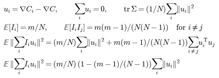
Dividing by m squared gives the noise of the batch gradient:

With replacement the second factor disappears and the noise is tr Σ / m. The noise falls like 1 / m while the cost of a step grows like m, and without replacement it vanishes for a batch of the whole data. The batch gradient must be the mean, not the sum, or the effective learning rate changes with the batch size.

How much a step gains, and the batch size

How useful is a less noisy gradient? Expand the cost to second order around θ, write G for the true gradient there, and average over the batch, using that the expected outer product of g with itself is G times its transpose plus Σ / m when sampling with replacement:

Minimizing over η gives the best step and the best expected gain:

If the curvature is about the same in all directions, the critical batch size reduces to the noise scale, the batch size at which the noise tr Σ / m equals the squared length of the true gradient (McCandlish et al., 2018):

Two regimes follow. For m much smaller than B the gain per step is proportional to m and so is the best step: doubling the batch doubles the progress per step at the same progress per example, and the learning rate should double with it, the linear scaling rule (Goyal et al., 2017). For m much larger than B the gain saturates and extra examples are wasted. If S min is the number of steps needed with exact gradients, a batch of m needs S steps and E examples in all:

The noise scale is not a constant: as training proceeds the true gradient shrinks while the per-example gradients do not, so B grows and larger batches become worthwhile. With a constant η the noise also keeps the iterate hopping around the minimum at an excess cost proportional to η tr Σ / m, which is the reason for the schedules below.

Momentum as an exponential average

SGD with momentum, in the form PyTorch uses, keeps a velocity:

Unrolling the recursion shows what the velocity is:

It is a sum of all past gradients with geometrically decaying weights and a memory of about 1 / (1 - β) steps, 10 for β = 0.9. Two consequences can be read off:

A constant gradient produces steps that approach the terminal velocity ηg / (1 - β), ten times the gradient-descent step for β = 0.9, while a gradient component that alternates in sign leaves a velocity of about half a single gradient. Momentum amplifies consistent directions by up to 1 / (1 - β) and damps oscillating ones.

The exponential-moving-average form has weights that sum to 1 - β to the power t, so its velocity is a true average and its steps are 1 - β times shorter; the same trajectory needs a learning rate 1 / (1 - β) times larger:

PyTorch's dampening d multiplies the new gradient by 1 - d, so dampening=beta gives this form, except that PyTorch starts the buffer at the first gradient, undamped.

The heavy ball

Momentum is a discretized physical system. A ball of unit mass moving in the potential C with friction coefficient γ obeys the first equation below. Replacing the derivatives by differences over a time step h and solving for the new position gives the other two lines:

This is Polyak's heavy-ball method with η = h² and β = 1 - γh: the momentum coefficient is one minus the friction per step. With β = 0 the friction is so strong that the ball has no memory and the method is gradient descent; as β approaches 1 the friction vanishes and the ball oscillates for ever. Writing each displacement as minus η times the velocity and substituting gives exactly the velocity update above, so PyTorch's momentum is the heavy ball (test_pytorch_momentum_is_the_heavy_ball checks it step by step).

Momentum on an ill-conditioned quadratic

On the quadratic with Hessian H, let x be the component of the error along an eigenvector with eigenvalue λ. Since the gradient is H times the error, the heavy-ball recursion becomes a scalar one of second order, and solutions of the form r to the power t require r to solve a quadratic equation:

The two roots multiply to β. When the discriminant is negative they are complex conjugates of equal size, so every such component shrinks by exactly √β per step, whatever its eigenvalue. The discriminant is negative inside a band of curvatures:

Choose η and β so that the whole spectrum fits the band, with λmin at its lower edge and λmax at its upper edge. Taking square roots of the two conditions and adding and subtracting them gives the tuned values:

The best gradient descent shrinks the error by (κ - 1) / (κ + 1), about 1 - 2 / κ, per step; the tuned heavy ball by about 1 - 2 / √κ. The number of steps for a tenfold reduction, ln 10 divided by minus the logarithm of the factor, is 115.1 for gradient descent and 11.5 for the heavy ball at κ = 100, and 11512.9 against 115.1 at κ = 10⁴. Complex roots mean the component oscillates while it shrinks: the tuned heavy ball spirals into the minimum, which is the overshooting seen in every momentum trajectory below. With β below the tuned value the flat or the steep direction falls outside the band and converges more slowly; above it, every component spirals at the slower rate √β. In general the recursion is stable when

so momentum also tolerates learning rates up to 1 + β times the gradient-descent limit.

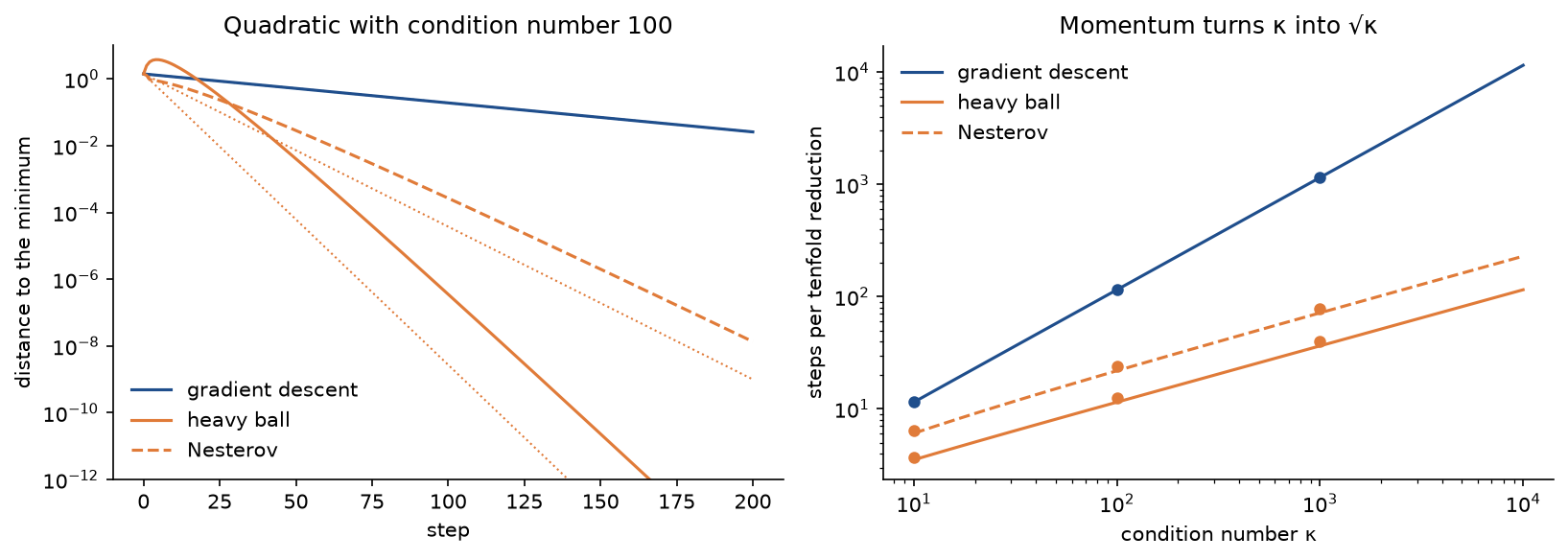
The figure, from examples/momentum_on_quadratic.py, confirms the theory on the quadratic with curvatures 1 and 100. Measured between steps 100 and 200, the contraction per step is 0.9802 for gradient descent at its best step η = 0.0198, 0.8238 against a predicted 0.8182 for the tuned heavy ball (η = 0.0331, β = 0.6694), and 0.9058 against 0.9000 for Nesterov (η = 0.01, β = 0.8182). The momentum methods measure slightly slower than their spectral radius because their repeated or nearly repeated roots add a factor growing like t. Scanning β at the heavy ball's η shows the band: β = 0, 0.3 and 0.5 diverge with factors 2.3058, 1.8430 and 1.4643, because this η exceeds the gradient-descent limit 2 / λmax = 0.02; from the tuned value upwards the factor equals √β, that is 0.8182, 0.8944, 0.9487 and 0.9747 for β = 0.6694, 0.8, 0.9 and 0.95. In the right panel the slopes are one and one half on logarithmic axes: momentum turns κ into √κ.

In deep learning β = 0.9 is the usual default; on a quadratic it is the tuned value for κ of about 1440, and for better-conditioned problems it trades some speed for robustness. With noisy gradients the acceleration largely disappears: for small learning rates SGD with momentum behaves like SGD with the learning rate η / (1 - β), and the benefit of momentum in networks comes as much from averaging the noise and moving faster through flat regions as from the √κ effect.

Nesterov momentum

Nesterov's method evaluates the gradient at the point the momentum is about to carry the parameters to:

Implementations store the look-ahead point ψ instead, where the next gradient is taken. Substituting the definitions and collecting terms turns the update into one that needs only gradients at the stored point:

The inner bracket is the new velocity, so the stored update is

which is torch.optim.SGD(nesterov=True). Compared with the heavy ball, the step uses the fresh gradient once more on top of the updated velocity, a correction applied before the overshoot rather than after it. On the quadratic its recursion is

With the standard choice η = 1 / λmax and β = (√κ - 1) / (√κ + 1), the steepest component vanishes after two steps and the flattest one has a double root at 1 - 1 / √κ: a factor 0.9 and 21.9 steps per tenfold reduction at κ = 100. That is half the speed of the tuned heavy ball on a quadratic, but Nesterov's rate is guaranteed for every smooth strongly convex function, while the heavy ball tuned for a quadratic can fail to converge on some that are not quadratic (Lessard, Recht and Packard, 2016).

AdaGrad

AdaGrad keeps the sum of all squared gradients and divides by its root:

Each coordinate effectively has its own learning rate, η divided by the root of the sum of its squared gradients. Three properties follow from the formula.

• Scale invariance per coordinate. Multiplying every gradient of a coordinate by a constant multiplies both g and the root of s by its size, so the steps do not change. In particular the first step is η times the sign of the gradient in every coordinate, however steep or flat, up to ε.
• A decaying step. A coordinate whose gradients have a constant size gets steps η / √t. Their sum grows like 2η√t, so the parameter can still travel any distance, but ever more slowly.
• Large steps for rare features. A coordinate that receives a gradient only occasionally keeps a small s and takes large steps when it does, which made AdaGrad popular for sparse problems such as word features.

AdaGrad is the diagonal version of a preconditioner, the inverse square root of the summed outer products of the gradients, derived from a regret bound in online convex optimization (Duchi, Hazan and Singer, 2011). Its weakness for networks is the same as its strength: the sum only grows, so the learning rate decays towards zero whether or not training needs it to.

RMSProp

RMSProp replaces the sum by an exponential moving average, so that old gradients are forgotten with a time constant of 1 / (1 - ρ) steps:

For gradients of steady size the root of s approaches that size and the step tends to η times a number of order one: the learning rate sets the step length directly, independent of the scale of the gradients. The average starts at zero, though, and for a constant gradient it has only reached a fraction of its final value:

The first steps are therefore longer than in the long run: 3.1623 times at the first step for ρ = 0.9 and 10 times for ρ = 0.99, PyTorch's default. PyTorch's RMSprop has no correction for this, and offers two extensions: a momentum buffer of normalized gradients, and a centered variant that divides by an estimate of the standard deviation rather than the root mean square. RMSProp was proposed by Tieleman and Hinton in 2012 and circulated without a paper.

Adam and its bias correction

Adam keeps exponential averages of the gradient and of its square, corrects both for having started at zero, and steps by their ratio, with the defaults β1 = 0.9, β2 = 0.999 and ε = 10⁻⁸:

The diagram traces one step from the gradient to the new parameters. The correction follows from unrolling the first average. If every gradient has the same expectation μ, the weights of the unrolled sum add up to 1 - β1 to the power t:

So v underestimates μ by the factor 1 - β1 to the power t, and v̂ removes the bias exactly. The same argument with the expectation of the squared gradient gives ŝ. When the expectations drift, the correction is exact for the steady part and close for slow drifts, because old terms carry geometrically small weights. Its effect is largest at the start: for a constant gradient v̂ equals g and ŝ equals its square at every step, so every step is η times the sign of g, while without the correction the step would be longer by the factor

With the defaults that factor is 3.1623 at the first step, peaks at 6.5685 at step 12, is still 1.2576 at step 1000 and reaches 1 only after several thousand steps.

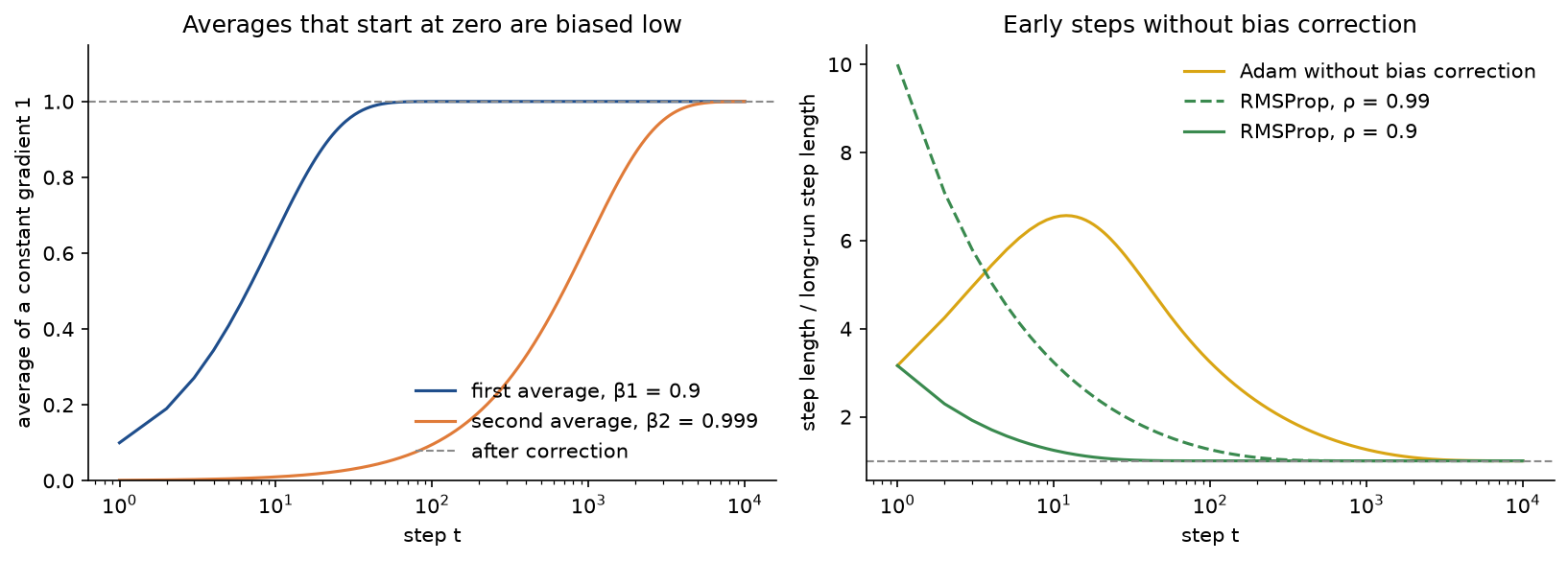
The figure, from examples/adaptive_steps.py, shows why the correction exists and what happens without it. Averages started at zero reach the true value only after a few times 1 / (1 - β) steps, about 30 steps for β1 = 0.9 and thousands for β2 = 0.999. Without correction Adam's early steps are inflated by up to 6.5685 times in a bump that lasts hundreds of steps, a warmup in reverse; RMSProp, which never had a correction, starts 10 times too long with ρ = 0.99. Learning-rate warmup is the usual remedy for the latter.

What Adam's step means:

• The ratio v̂ / √ŝ estimates the mean of the gradient divided by its root mean square, which lies between -1 and 1. When the gradient of a coordinate is consistent the step is about η; when it is mostly noise the step shrinks. Adam anneals itself where the gradient is noisy, and its learning rate is in units of parameter change, not of gradient.
• Like AdaGrad and RMSProp it is invariant to rescaling the cost or any one coordinate's gradient, up to ε. On a quadratic with a diagonal Hessian its iterates therefore do not depend on the curvatures at all, only on the starting point.
• Adam is RMSProp with the gradient replaced by a moving average, which is momentum in the exponential-average form, plus bias correction for both averages.
• The constant ε matters when the root of ŝ is comparable to it; for very small gradients Adam turns into momentum SGD with learning rate η / ε.

Reddi, Kale and Kumar (2018) showed that Adam can fail to converge on simple convex problems because ŝ can shrink and enlarge the steps again; their AMSGrad variant divides by the running maximum of s (amsgrad=True in PyTorch).

Weight decay and AdamW

An L2 penalty adds λ/2 times the squared length of θ to the cost and λθ to the gradient. For plain SGD the two descriptions are the same update:

The penalty multiplies every weight by 1 - ηλ before the gradient step, which is what weight decay means. (Regularization covers the penalty and its effect on generalization.) In an adaptive method the two are no longer the same. Adam with an L2 penalty feeds g + λθ into both averages, so the shrinking part of its step is divided by the same denominator as the data part:

A weight whose gradients are large or noisy, with a large ŝ, is barely regularized, while a weight that receives no gradient from the data has g = λθ, a ratio v̂ / √ŝ near the sign of θ, and moves towards zero at roughly η per step whatever λ is. Loshchilov and Hutter (2019) proposed to decouple the two:

AdamW shrinks every weight by the same factor at every step, independently of its gradient history, and makes the learning rate and the regularization strength separate knobs. In PyTorch the decay per step is lr * weight_decay with lr including any schedule; the paper multiplies λ by the schedule's multiplier only, so PyTorch's weight_decay corresponds to the paper's λ divided by the base learning rate.

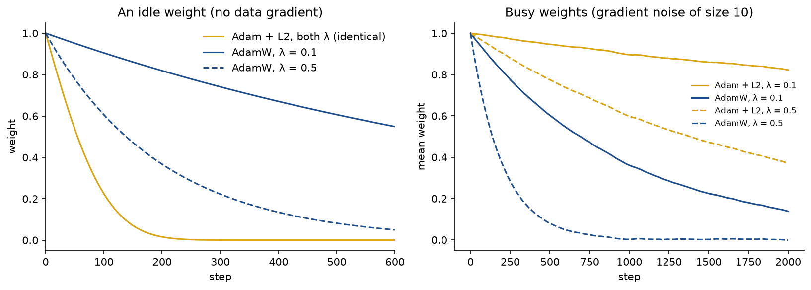
The figure, from examples/adaptive_steps.py, makes the difference visible with two kinds of weights started at 1 with η = 0.01: an idle weight whose data gradient is zero, and 2000 busy weights whose data gradients are pure noise of standard deviation 10.

• Adam with L2, λ = 0.1: the idle weight is 0.5368 after 50 steps, 0.2244 after 100 and 0.0000 after 2000; the mean busy weight after 2000 steps is 0.8223.
• AdamW, λ = 0.1: the idle weight is 0.9512, 0.9048 and 0.1352; the mean busy weight is 0.1384.
• Adam with L2, λ = 0.5: the idle weight follows exactly the same path, 0.5368, 0.2244 and 0.0000; the mean busy weight is 0.3707.
• AdamW, λ = 0.5: the idle weight is 0.7783, 0.6058 and 0.0000; the mean busy weight is -0.0011.

The idle weight under Adam with L2 follows the same path for both values of λ, because its only gradient is λθ and Adam ignores the scale of a gradient; it is near zero after about 250 steps, somewhat slower than η per step because ŝ remembers the larger early gradients. The busy weights barely decay under Adam with L2: their denominator is the noise level 10, so the decay rate is ηλ / 10, and the mean after 2000 steps, 0.8223 for λ = 0.1, is close to the exponential of -0.2, 0.8187. AdamW shrinks both kinds by 1 - ηλ per step, and 0.999 to the power 2000 is 0.1352 for λ = 0.1. In a network this means that with Adam and an L2 penalty, weights that receive little gradient are driven to zero at a speed set by η rather than λ, while weights with large or noisy gradients are hardly regularized: λ no longer controls what it is meant to control. For plain SGD the two forms agree to within 8.9 × 10⁻¹⁶ after 50 steps.

Learning-rate schedules

A schedule sets the learning rate as a function of the number k of steps already taken; step t uses the value at k = t - 1, the convention of torch.optim.lr_scheduler, whose step() is called after each optimizer.step(). With a base rate η0 and T steps in all, the common schedules are

The one-cycle policy (Smith and Topin, 2019) interpolates with half cosines, rising for the first fraction p of the steps and falling for the rest:

PyTorch's defaults are p = 0.3, d = 25 and a final divisor of 10⁴. The momentum, or Adam's β1, moves the opposite way, from 0.95 down to 0.85 and back, so that the total push η / (1 - β) changes less abruptly. Cosine annealing is periodic in k: continued past T, its learning rate climbs back up, which is the basis of warm restarts (Loshchilov and Hutter, 2017) and a frequent bug.

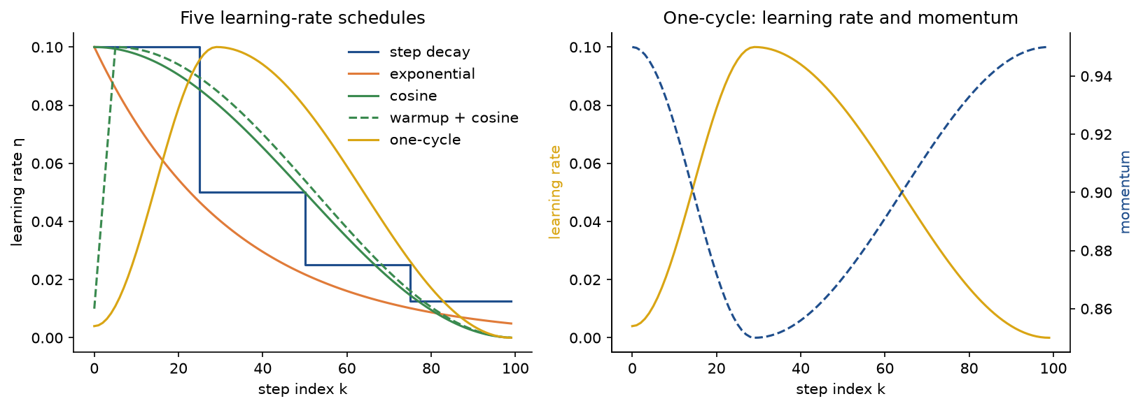
The figure, from examples/schedules_and_clipping.py, shows the five schedules with a base or peak rate of 0.1: step decay halving every 25 steps, exponential decay by 0.97 per step, cosine annealing to zero, five steps of warmup from 0.01 followed by cosine annealing, and one-cycle from 0.004 up to 0.1 at index 29 and down to 4 × 10⁻⁷. Every value agrees with torch.optim.lr_scheduler (StepLR, ExponentialLR, CosineAnnealingLR, LinearLR and CosineAnnealingLR joined by SequentialLR, and OneCycleLR) to within 6.9 × 10⁻¹⁷, including the momentum or β1 that OneCycleLR cycles.

The reasons for a schedule come from the sections above. With noisy gradients a constant η leaves an excess cost proportional to η, so the rate must decrease to settle; the conditions of Robbins and Monro describe decays that reach the minimum in the limit:

Early on a large rate makes fast progress, and in networks it also tends to find flatter regions. Warmup protects the first steps: Adam's first ŝ is a single squared gradient, so its first step sizes are erratic until enough samples have been averaged (Liu et al., 2020), and with large batches the early curvature can be too high for the target learning rate (Goyal et al., 2017).

The learning-rate range test

The range test (Smith, 2017) runs one short training session in which the learning rate rises exponentially, one mini-batch per value. The batch costs are smoothed with an exponential average and divided by its correction for the same reason as in Adam, and the run stops once the smoothed cost exceeds four times its minimum:

Plotted against η on a logarithmic axis, the cost is flat while the rate is too small to matter, falls, reaches a minimum and then explodes. The usual readings are a constant learning rate of one tenth of the rate at the minimum, or the rate where the cost falls fastest, and a one-cycle peak near the minimum itself, the largest rate that still makes progress. Each rate is used for a single mini-batch, on weights trained by the smaller rates before it, so the test measures short-term progress only; the sample project compares it with a full sweep.

Gradient clipping

Clipping by global norm computes the length of all gradients taken together and rescales them, with the small constant that torch.nn.utils.clip_grad_norm_ adds:

The direction is kept and an SGD step can never be longer than ηc. Clipping by value clamps each entry to the interval from -c to c and changes the direction. Gradients explode because backpropagation multiplies one Jacobian per layer, or per time step in a recurrent network, which multiplies by the same weight matrix again and again: B2 unrolled through T steps contains the T-th power of that matrix. The cost surface then has cliffs, narrow regions where the gradient is orders of magnitude larger than nearby, and one unclipped step there can throw the parameters arbitrarily far (Pascanu, Mikolov and Bengio, 2013). Adam's steps are normalized, but a spike still enters s and inflates the denominator for about 1 / (1 - β2) steps, so clipping before the optimizer also protects its statistics. Clipping bounds the damage of a step; it does not make a learning rate that is too large for the local curvature converge.

A linear recurrent unit with one weight w, run for ten steps from a hidden state of 1, outputs w to the power 10, and its cost has the cliff described above:

The minimum is at w = 1.0718, the gradient is tiny for w below 1 and explosive just above w, and the curvature at the minimum, 348.2, caps any constant learning rate that is to settle there at 2 / 348.2 = 0.0057. Five runs start from w = 0.5, and after 10, 11, 12 and 13 steps they stand at:

• η = 0.2: 0.9335, 2.5459, -1.028 × 10⁸ and 3.4 × 10¹⁵², after which the cost overflows.
• η = 0.2, clipped at norm 1: 0.9227, 1.1227, 0.9227 and 1.123; the cost is still 1.21 after 50 and after 150 steps.
• η = 0.005: 0.5020, 0.5022, 0.5024 and 0.5026; after 150 steps w has crept only to 0.5410, with the cost still about 2.
• η = 0.2 times 0.96 to the power k: 0.6853, 0.7730, 1.015 and 2.192, after which the cost overflows.
• The same decaying rate, clipped at norm 1: 0.6853, 0.7730, 0.9006 and 1.023; the cost is 0.0786 after 50 steps and 2.2 × 10⁻³¹ after 150.

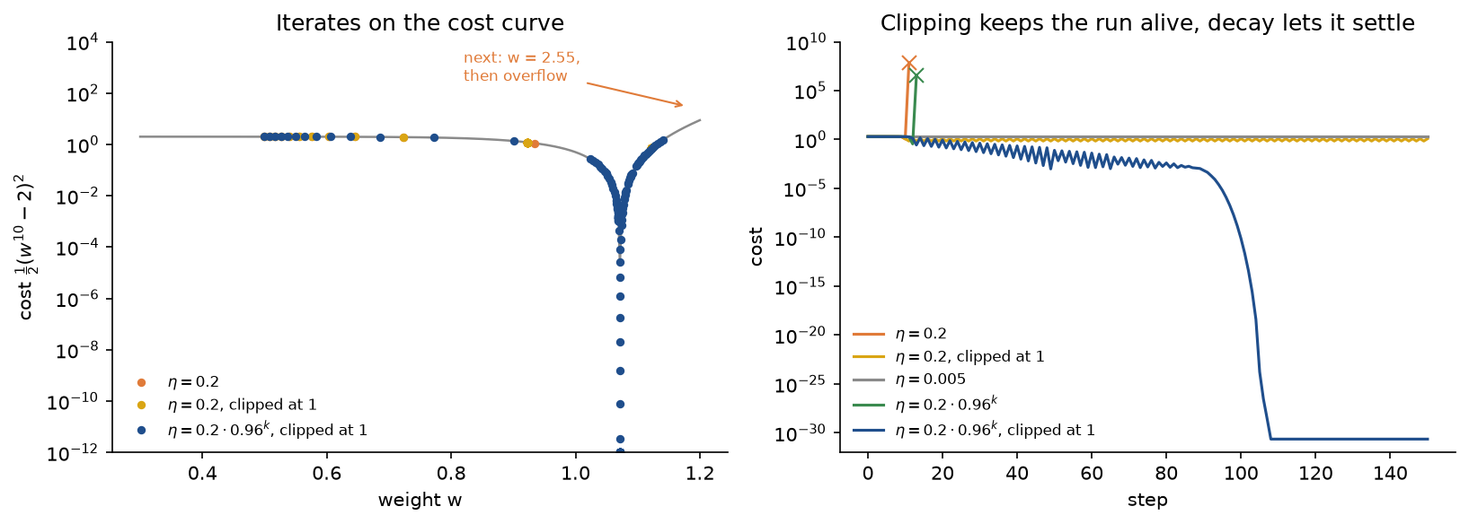
The figure, from examples/schedules_and_clipping.py, shows the runs. The unclipped run approaches the cliff, is catapulted from 0.9335 to 2.5459, then to about -10⁸, and overflows. A learning rate small enough for the minimum, 0.005, has barely moved after 150 steps. Clipping alone keeps the run alive but leaves it bouncing between 0.9227 and 1.1227 for ever, because 0.2 is far above the stability limit; decay alone still meets the cliff while the rate is large. Only the two together converge, to the minimum in double precision, with a cost below 10⁻³⁰ from step 108.

Saddle points and curved valleys

At a saddle point the gradient vanishes and the Hessian has negative eigenvalues. Near it, gradient descent multiplies the component along a direction of curvature -μ by 1 + ημ per step, so starting a distance δ from the attracting directions it needs about

steps to leave: slow when δ is small. Momentum accumulates the escaping component, and the adaptive methods divide the tiny component by its own tiny size and escape at once. In high dimensions most critical points with a high cost are saddles rather than local minima (Dauphin et al., 2014), which makes this behaviour more relevant than local minima. The three test surfaces below show an ill-conditioned valley, a curved valley and a saddle:

The quadratic has curvatures 1 and 20, and a copy of it rotated by 45 degrees is the same problem in turned coordinates. The Rosenbrock function's Hessian at its minimum (1, 1) has eigenvalues 1001.6006 and 0.3994, a condition number of about 2508, and the direction of the valley floor turns as the path follows it. The saddle has its saddle point at the origin and minima at (0, 1) and (0, -1). examples/trajectories.py runs six optimizers on each, with settings chosen to show each method's character rather than tuned to win:

• On both quadratics, from (-4, 1.5) and its rotation, for 80 steps: gradient descent with η = 0.09, momentum and Nesterov with η = 0.04 and β = 0.8, AdaGrad with η = 1, RMSProp with η = 0.1 and ρ = 0.9, Adam with η = 0.2.
• On Rosenbrock, from (-1.5, 2), for 1500 steps: gradient descent with η = 0.0007, momentum and Nesterov with the same η and β = 0.9, AdaGrad with η = 0.3, RMSProp with η = 0.003 and ρ = 0.9, Adam with η = 0.02.
• On the saddle, from (2, 0.001), for 80 steps: gradient descent with η = 0.1, momentum and Nesterov with the same η and β = 0.8, AdaGrad with η = 0.3, RMSProp with η = 0.03 and ρ = 0.9, Adam with η = 0.05.

AdamW is left out: without weight decay it is Adam, and with it the minimum itself moves.

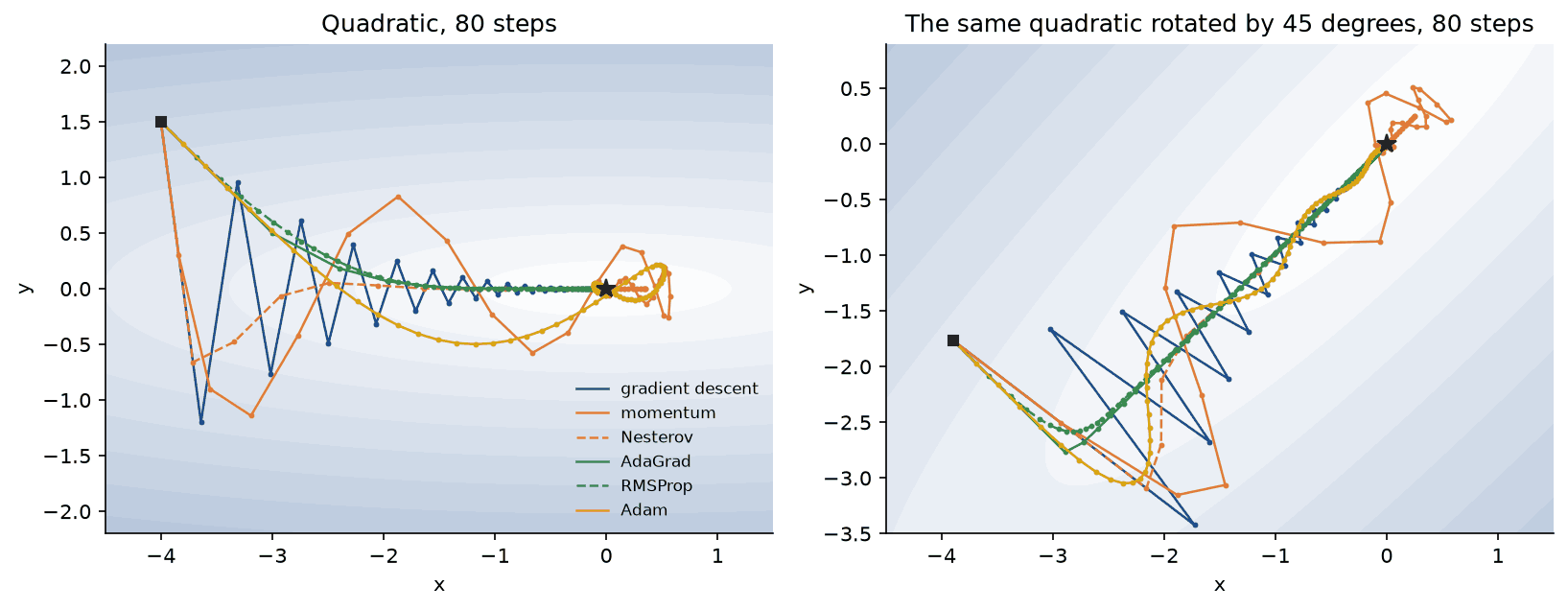
On the aligned quadratic gradient descent zigzags across the valley, momentum overshoots in wide loops, Nesterov damps them, AdaGrad and RMSProp head almost straight for the axis and then along it, and Adam, whose steps stay near η = 0.2, circles the minimum at the end. After 80 steps the costs are 2.24 × 10⁻⁶ for gradient descent, 4.69 × 10⁻⁷ for momentum, 5.10 × 10⁻⁹ for Nesterov, 1.84 × 10⁻¹¹ for AdaGrad, 1.01 × 10⁻¹⁶ for RMSProp and 9.13 × 10⁻⁴ for Adam. Rotating the problem leaves the first three unchanged, since they only combine gradients and a rotation turns every gradient with the parameters, but costs AdaGrad and RMSProp more than eight and ten orders of magnitude, 7.24 × 10⁻³ and 6.26 × 10⁻⁶, and Adam a factor of 1.7, 1.51 × 10⁻³. Per-coordinate scaling fixes ill-conditioning only along the axes.

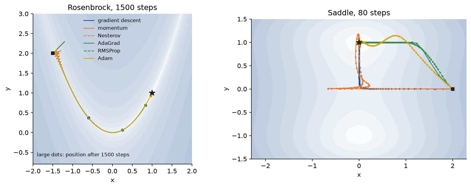
On Rosenbrock all six reach the curved valley quickly and then differ in how fast they follow it. After 1500 steps momentum and Nesterov stand at (0.9932, 0.9865) and (0.9930, 0.9861), with costs below 0.01 from steps 617 and 624, Adam at (0.9596, 0.9208) after reaching 0.01 at step 1247, RMSProp at (0.8327, 0.6888), AdaGrad, whose steps keep shrinking, at (0.2495, 0.0609), and gradient descent, held to η = 0.0007 by the steep walls, only at (-0.6024, 0.3707). At the saddle, gradient descent slides along the line y = 0 to within 0.0522 of the saddle point and needs 67 steps before the size of y exceeds 0.5; momentum and Nesterov escape after 28 and 25 steps. The adaptive methods never come near the saddle: they divide the tiny gradient in y by its own size, and AdaGrad, RMSProp and Adam pass 0.5 after 2, 7 and 11 steps.

Worked example

The cost is a quadratic of two parameters θ = (x, y) whose curvatures, 4 and 0.2, differ by a factor of 20:

Every method starts at θ₀ = (1, 2) with learning rate η = 0.1 and runs for three steps; momentum uses β = 0.9, RMSProp ρ = 0.9, and Adam its defaults. Values are computed in double precision and shown with four decimals; ε changes nothing at that precision. Vectors are written as (first coordinate, second coordinate), and a change is the new θ minus the old one.

Gradient descent

Gradient descent multiplies x by 1 - 0.1 × 4 = 0.6 and y by 1 - 0.1 × 0.2 = 0.98 at every step. The gradients are (4.0000, 0.4000), (2.4000, 0.3920) and (1.4400, 0.3842), and the iterates (0.6000, 1.9600), (0.3600, 1.9208) and (0.2160, 1.8824), with costs 1.1042, 0.6281 and 0.4476: the steep coordinate is almost done, the flat one has hardly moved.

Momentum and Nesterov

Momentum adds the gradient to 0.9 times the velocity and moves by 0.1 times the velocity:

• Step 1: gradient (4.0000, 0.4000), velocity (4.0000, 0.4000), change (-0.4000, -0.0400), θ (0.6000, 1.9600), cost 1.1042.
• Step 2: gradient (2.4000, 0.3920), velocity (6.0000, 0.7520), change (-0.6000, -0.0752), θ (0.0000, 1.8848), cost 0.3552.
• Step 3: gradient (0.0000, 0.3770), velocity (5.4000, 1.0538), change (-0.5400, -0.1054), θ (-0.5400, 1.7794), cost 0.8998.

At step 2 the velocity is 0.9 × (4, 0.4) + (2.4, 0.392) = (6, 0.752). In y, where the gradient keeps its sign, the steps grow from 0.04 to 0.0752 to 0.1054 on their way to the terminal 0.1 × 0.38 / (1 - 0.9), about 0.38. In x the velocity carries the parameter straight through the minimum: at step 3 the gradient in x is exactly zero, yet the step is -0.54, and the cost rises from 0.3552 to 0.8998. Momentum does not decrease the cost at every step.

Nesterov uses the same velocity but moves by 0.1 times the gradient plus 0.9 times the new velocity:

• Step 1: gradient (4.0000, 0.4000), velocity (4.0000, 0.4000), change (-0.7600, -0.0760), θ (0.2400, 1.9240), cost 0.4854.
• Step 2: gradient (0.9600, 0.3848), velocity (4.5600, 0.7448), change (-0.5064, -0.1055), θ (-0.2664, 1.8185), cost 0.4726.
• Step 3: gradient (-1.0656, 0.3637), velocity (3.0384, 1.0340), change (-0.1669, -0.1294), θ (-0.4333, 1.6891), cost 0.6608.

The first change is -0.1 × (4 + 0.9 × 4) = -0.76 in x, larger than the heavy ball's, because the update already contains the momentum step that the look-ahead anticipates. At step 3 the gradient in x has turned negative and cuts the step to -0.1669, where the heavy ball still moved by -0.54: the correction acts one step earlier.

AdaGrad

AdaGrad adds the squared gradient to s and moves by 0.1 times the gradient divided by the root of s:

• Step 1: gradient (4.0000, 0.4000), s (16.0000, 0.1600), change (-0.1000, -0.1000), θ (0.9000, 1.9000).
• Step 2: gradient (3.6000, 0.3800), s (28.9600, 0.3044), change (-0.0669, -0.0689), θ (0.8331, 1.8311).
• Step 3: gradient (3.3324, 0.3662), s (40.0650, 0.4385), change (-0.0526, -0.0553), θ (0.7805, 1.7758).

The first step divides each gradient by its own size, 4 by the root of 16 and 0.4 by the root of 0.16, and moves both coordinates by exactly 0.1 although their gradients differ by a factor of 10. At step 2, s = 16 + 3.6² = 28.96 and the change in x is 0.1 × 3.6 / 5.3814 = 0.0669. The steps then shrink, roughly like 1 / √t, because the sum keeps growing.

RMSProp

RMSProp keeps 0.9 times s plus 0.1 times the squared gradient and moves by 0.1 times the gradient divided by the root of s:

• Step 1: gradient (4.0000, 0.4000), s (1.6000, 0.0160), change (-0.3162, -0.3162), θ (0.6838, 1.6838).
• Step 2: gradient (2.7351, 0.3368), s (2.1881, 0.0257), change (-0.1849, -0.2099), θ (0.4989, 1.4739).
• Step 3: gradient (1.9955, 0.2948), s (2.3675, 0.0319), change (-0.1297, -0.1652), θ (0.3692, 1.3087).

The first average is a tenth of the squared gradient, so the first step is 0.1 × 4 / √1.6 = 0.1 / √0.1 = 0.3162 in both coordinates: 3.1623 times the learning rate, the start-up effect described above. At step 2 the gradient in x is 4 × 0.6838 = 2.7351 and s = 0.9 × 1.6 + 0.1 × 2.7351² = 2.1881, whose root is 1.4792, giving a change of 0.1 × 2.7351 / 1.4792 = 0.1849.

Adam

Adam keeps v as 0.9 v + 0.1 g and s as 0.999 s + 0.001 g², divides them by 1 - 0.9 to the power t and 1 - 0.999 to the power t, and moves by 0.1 times v̂ over the root of ŝ. The raw second averages are small, so they are shown multiplied by 1000:

• Step 1: gradient (4.0000, 0.4000), v (0.4000, 0.0400), 1000 s (16.0000, 0.1600), v̂ (4.0000, 0.4000), ŝ (16.0000, 0.1600), change (-0.1000, -0.1000), θ (0.9000, 1.9000).
• Step 2: gradient (3.6000, 0.3800), v (0.7200, 0.0740), 1000 s (28.9440, 0.3042), v̂ (3.7895, 0.3895), ŝ (14.4792, 0.1522), change (-0.0996, -0.0998), θ (0.8004, 1.8002).
• Step 3: gradient (3.2016, 0.3600), v (0.9682, 0.1026), 1000 s (39.1656, 0.4336), v̂ (3.5726, 0.3786), ŝ (13.0683, 0.1447), change (-0.0988, -0.0995), θ (0.7016, 1.7006).

Step 1: v = 0.1 g = (0.4, 0.04) and s = 0.001 g² = (0.016, 0.00016). Dividing by 1 - 0.9 = 0.1 and 1 - 0.999 = 0.001 gives back g and its square exactly, so the step is 0.1 times the sign of g, (-0.1, -0.1). Without the correction it would be 0.1 × 0.4 / √0.016 = 0.3162, the factor 3.1623 from the section on bias correction.

Step 2, first coordinate: the gradient is 4 × 0.9 = 3.6, v = 0.9 × 0.4 + 0.1 × 3.6 = 0.72 and s = 0.999 × 0.016 + 0.001 × 12.96 = 0.028944. The corrections divide by 1 - 0.81 = 0.19 and 1 - 0.998001 = 0.001999, giving v̂ = 3.7895 and ŝ = 14.4792, whose root is 3.8052. The change is 0.1 × 3.7895 / 3.8052 = 0.0996: the averaged gradient is slightly smaller than the averaged size because the gradient is shrinking. In the second coordinate the ratio is 0.3895 / 0.3901 and the change 0.0998.

Adam moves both coordinates by almost exactly the learning rate at every step, the flat one as fast as the steep one. Because of the per-coordinate scale invariance, the changes and iterates of AdaGrad, RMSProp and Adam would be the same for any other curvature in place of 0.2; only the gradients and their averages would differ (test_adaptive_iterates_ignore_the_curvature_of_each_coordinate).

After three steps

Where each method stands, with its cost, against 2.4 at the start:

• Gradient descent: (0.2160, 1.8824), cost 0.4476.
• Momentum: (-0.5400, 1.7794), cost 0.8998.
• Nesterov: (-0.4333, 1.6891), cost 0.6608.
• AdaGrad: (0.7805, 1.7758), cost 1.5336.
• RMSProp: (0.3692, 1.3087), cost 0.4439.
• Adam: (0.7016, 1.7006), cost 1.2737.
• Adam without bias correction: (-0.1621, 0.7829), cost 0.1139.
• AdamW with λ = 0.1: (0.6751, 1.6444), cost 1.1819.

Three steps say little about which method wins in the long run, but they show each method's character. Gradient descent and the momentum methods are dominated by the steep coordinate; the adaptive methods move the flat coordinate as far as the steep one. Adam without bias correction happens to be lowest here because its early steps are 3 to 5 times longer, which helps on a convex bowl and is exactly what destabilizes the first steps of a network. AdamW first multiplies θ by 1 - 0.1 × 0.1 = 0.99 and then takes Adam's step, so its first change is (-0.1100, -0.1200). Every number in this section is printed by examples/worked_steps.py and asserted by tests/test_worked.py, tests/test_sgd.py, tests/test_adaptive.py and tests/test_adam.py.

The code

The package optimizers is plain NumPy, split into one module per idea. PyTorch is imported only inside the functions of comparisons.py and torch_training.py, so everything else works without it.

• The update rules. arrays.py holds the parameter types, a tuple of arrays in the order of torch.nn.Sequential.parameters(), and state.py the frozen State with the step count and the buffers v and s. sgd.py holds SGD with momentum, dampening, Nesterov and either kind of weight decay; adaptive.py holds Adagrad and RMSprop with its momentum and centered options; adam.py holds Adam, AdamW and the start-up factors of the bias-correction section. Each optimizer's step(parameters, gradients, state) returns new parameters and a new state.
• Steering the step. schedules.py holds StepDecay, ExponentialDecay, CosineAnnealing, WarmupCosine and OneCycle, each with learning_rate(k) and momentum(k); clipping.py holds global_norm, clip_by_global_norm and clip_by_value; running.py holds configure, which applies a schedule to an optimizer for step k, and run, which drives any function returning a cost and gradients and records a Trajectory.
• Analysis on test problems. surfaces.py holds the quadratic, Rosenbrock, saddle and recurrent-unit costs; convergence.py the iteration matrices, the tuned settings and the measured contraction of the momentum section; landscapes.py, decay.py and cliff.py build the experiments behind the trajectory, weight-decay and clipping figures.
• The worked example. worked.py builds the problem and the eight optimizers of the worked example, and trace.py records every intermediate quantity of a few steps as StepRecords and prints them with format_trace.
• The network. datasets.py generates the three spirals; network.py holds the tanh network with a softmax output, its cross-entropy, B1 to B4 in the row layout and per-example gradients; noise.py the noise formula, its brute-force check and the noise scale; training.py mini-batch training with a fixed batch order, schedule and clipping; range_test.py the range test and its readings.
• The benchmark. benchmark.py holds the optimizer list, the learning-rate grid, the sweep, the range tests, the twelve configurations and their summaries; batch_study.py the noise-scale and batch-size studies.
• Checks and comparisons. problems.py holds the random problems and configuration lists the tests share; pitfalls.py the computations behind the Pitfalls section; comparisons.py builds the matching torch.optim optimizer and scheduler and replays a run through them; torch_training.py trains the network with autograd and demonstrates two PyTorch mistakes.
• Figures. plotting.py holds the four colours, one colour and line style per method and reproducible saving; step_plots.py, surface_plots.py and benchmark_plots.py draw every figure on this page onto axes they are given, so the notebook can show the same plots inline.

Every optimizer follows PyTorch's arithmetic, including its quirks: the momentum buffer starts at the first gradient, ε is added after the square root, and AdamW decays by learning_rate * weight_decay. Adam's step in adam.py is the formula almost symbol for symbol:

first = previous_first + (1.0 - self.beta1) * (gradient - previous_first)
second = previous_second * self.beta2 + (1.0 - self.beta2) * gradient * gradient
denominator = np.sqrt(second) / root_correction + self.epsilon
updated.append(parameter - step_size * first / denominator)

Here step_size is η divided by 1 - β1 to the power t and root_correction is the root of 1 - β2 to the power t. The worked example's Adam steps are reproduced by

from optimizers import Adam, format_trace, worked_trace

print(format_trace(worked_trace(Adam(0.1)), square_scale=1000.0))

The examples and the project import the package, so install the repository first as described in the main README. Each example demonstrates one idea and runs from the repository root in about a second, the comparison with PyTorch in about fifteen:

• examples/worked_steps.py prints every value of the worked example, method by method, then where all eight variants stand after three steps.
• examples/momentum_on_quadratic.py computes the tuned settings, the predicted and measured contraction and the scan over β, and saves figures/momentum-quadratic.png.
• examples/trajectories.py runs six optimizers on the four surfaces, prints final costs, the effect of rotation, the saddle escapes and the progress along the Rosenbrock valley, and saves both trajectory figures.
• examples/adaptive_steps.py prints the start-up factors of RMSProp and uncorrected Adam, runs the weight-decay experiment, and saves figures/bias-correction.png and figures/weight-decay.png.
• examples/schedules_and_clipping.py prints the five schedules, the misuses of a cosine schedule, three momentum conventions under a rate drop and the five runs on the recurrent cliff, and saves figures/schedules.png and figures/clipping.png.
• examples/compare_with_pytorch.py checks every optimizer and schedule against PyTorch, from the worked example to full training runs, and demonstrates two PyTorch mistakes.

python neural-networks/optimizers/examples/worked_steps.py
python neural-networks/optimizers/examples/momentum_on_quadratic.py
python neural-networks/optimizers/examples/trajectories.py
python neural-networks/optimizers/examples/adaptive_steps.py
python neural-networks/optimizers/examples/schedules_and_clipping.py
python neural-networks/optimizers/examples/compare_with_pytorch.py

The sample project: a fair optimizer benchmark

project/optimizer_benchmark.py asks the question every optimizer comparison should answer: which optimizer and schedule train one given network best, when each gets its own tuned learning rate and is judged over several seeds?

The data are three interleaved spiral arms of 300 points each, with Gaussian noise of 0.5 radians in the angle so that the arms overlap and no classifier is perfect, standardized with the training mean and standard deviation; a second draw with the next seed is the test set. The network is 2-32-32-3 with tanh hidden units and a softmax output, 1251 parameters, trained on cross-entropy in mini-batches of 32 for 60 epochs, 1740 steps. It starts at a cost of 1.3132. Options such as --samples, --noise, --hidden, --epochs, --batch-size and --seeds change the setup, --skip-batch-study leaves out the last stage, and --figures sends the PNGs to another folder so a custom run does not overwrite the ones shown here. The default run takes about 30 seconds on one CPU thread.

python neural-networks/optimizers/project/optimizer_benchmark.py
python neural-networks/optimizers/project/optimizer_benchmark.py --seeds 5 --skip-batch-study

First, every optimizer is trained once per learning rate on the grid 0.001, 0.003, 0.01, 0.03, 0.1, 0.3, 1 and 3, from the same initial weights. The final training costs, in that order, are:

• SGD: 1.0305, 0.9958, 0.8589, 0.5685, 0.3493, 0.1443, 0.1904 and 10.50; best at 0.3.
• Momentum: 0.8607, 0.5509, 0.3501, 0.1509, 0.1490, 2.6365, 3.0099 and 60.17; best at 0.1.
• Nesterov: 0.8604, 0.5499, 0.3240, 0.1401, 0.1691, 0.4804, 21.05 and 21.39; best at 0.03.
• AdaGrad: 1.0040, 0.9072, 0.6091, 0.4515, 0.1529, 0.0859, 0.1348 and 0.3243; best at 0.3.
• RMSProp: 0.5094, 0.3464, 0.1047, 0.2967, 0.4177, 7.7237, 19.72 and 95.80; best at 0.01.
• Adam: 0.4825, 0.2824, 0.1686, 0.1294, 0.4961, 2.0652, 3.9034 and 25.96; best at 0.03.
• AdamW with weight decay 0.01: 0.4861, 0.2915, 0.1809, 0.1737, 0.4685, 1.3545, 2.4172 and 9.5210; best at 0.03.

The best learning rates span a factor of 30, from 0.01 for RMSProp to 0.3 for SGD and AdaGrad, and every optimizer's final cost rises by at least 60 % two grid points away from its best, usually by far more. A comparison at one shared learning rate would mostly measure which optimizer happens to like that rate.

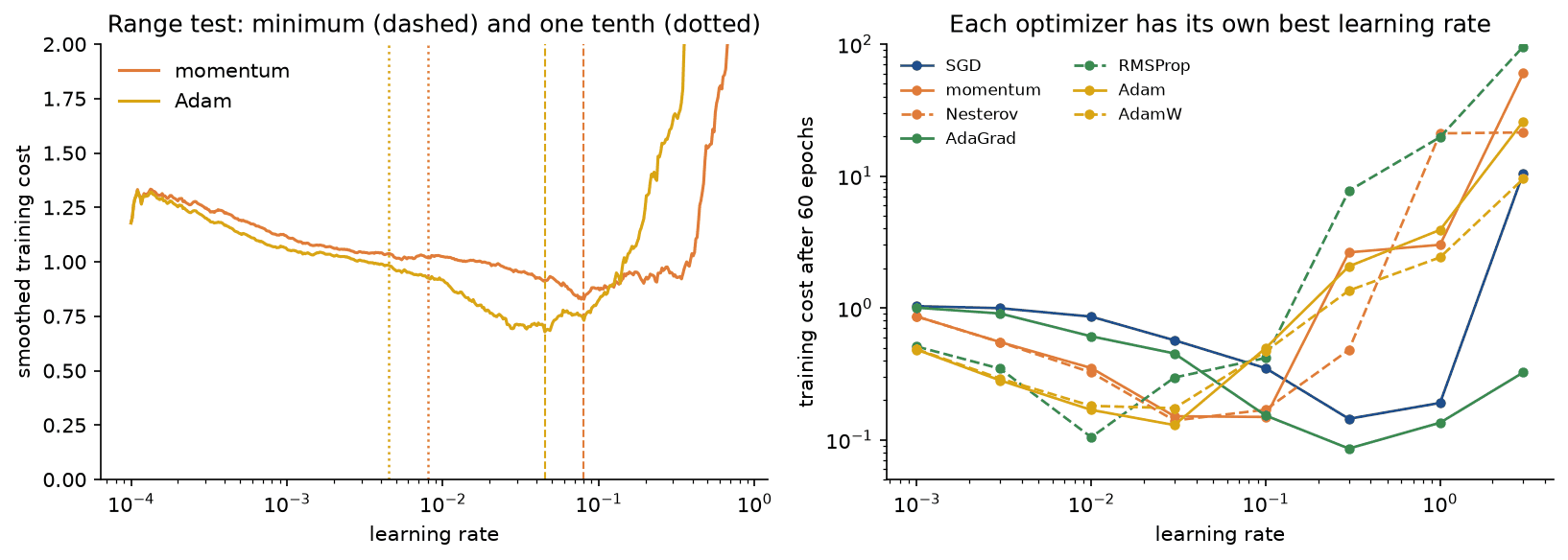
The range test for momentum stopped after 467 steps at a rate of 0.776, with its minimum at 0.0803 and its steepest descent at 0.0676; for Adam it stopped after 433 steps at 0.404 with the minimum at 0.0451. On this problem the minima land within a factor of 1.5 of the sweep's best constant rates, 0.1 and 0.03, at the cost of one short run instead of eight full ones, while the one-tenth rule, 0.0080 and 0.0045, is a factor of 7 to 13 too cautious. The cost curve also explains the shape of the sweep: below about 0.01 the cost falls only slowly within a few hundred steps, and the explosion begins a factor of 3 to 10 above the minimum.

Next, each optimizer runs at its best grid rate, and five schedules are added: step decay by 0.2 after each third of training, cosine annealing and one-cycle for momentum, and warmup over the first 5 % of steps followed by cosine annealing, and one-cycle, for Adam. Step decay and the cosine schedules start from the best constant rate; the one-cycle peaks are the range-test minima. Every configuration runs with three seeds, which change the initial weights and the batch order. For each, the medians over the seeds of the training cost after 10 and 60 epochs, the worst seed's final cost, and the medians of the test cost and test accuracy are:

• SGD at 0.3: 0.6336, 0.1491, worst 0.1802; test cost 0.1914, accuracy 0.9300.
• Momentum at 0.1: 0.4654, 0.1587, worst 0.2118; test cost 0.2505, accuracy 0.9144.
• Nesterov at 0.03: 0.5241, 0.1493, worst 0.1503; test cost 0.1809, accuracy 0.9378.
• AdaGrad at 0.3: 0.2802, 0.0904, worst 0.1008; test cost 0.1694, accuracy 0.9378.
• RMSProp at 0.01: 0.3699, 0.1134, worst 0.1242; test cost 0.1785, accuracy 0.9400.
• Adam at 0.03: 0.3731, 0.2041, worst 0.2921; test cost 0.2925, accuracy 0.9000.
• AdamW at 0.03: 0.3928, 0.2080, worst 0.2264; test cost 0.2445, accuracy 0.9222.
• Momentum with step decay: 0.4654, 0.1049, worst 0.1242; test cost 0.1655, accuracy 0.9433.
• Momentum with cosine annealing: 0.4994, 0.0944, worst 0.1095; test cost 0.1537, accuracy 0.9433.
• Momentum with one-cycle to 0.0803: 0.6959, 0.1027, worst 0.1186; test cost 0.1564, accuracy 0.9467.
• Adam with warmup and cosine: 0.4413, 0.0950, worst 0.0981; test cost 0.1523, accuracy 0.9400.
• Adam with one-cycle to 0.0451: 0.6199, 0.0933, worst 0.0980; test cost 0.1672, accuracy 0.9411.

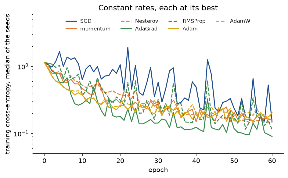
With constant learning rates all seven stall at a noise floor between about 0.09 and 0.21 and jump around it from epoch to epoch. The adaptive methods make the fastest early progress, 0.28 to 0.39 after 10 epochs against 0.47 to 0.63 for the SGD family. AdaGrad ends lowest among the constant rates because its effective rate decays like 1 / √t, which is a schedule in disguise. Adam at its sweep-best rate is the noisiest of all, with a worst seed 43 % above its median.

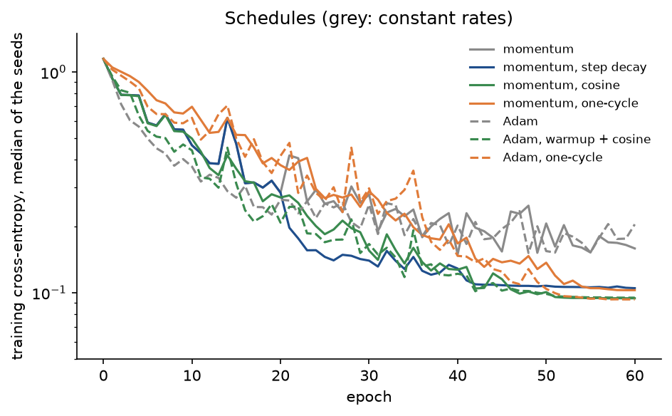
Every schedule removes the floor: the five end between 0.0933 and 0.1049, with the worst seed never more than 0.02 above the median, and their test costs, 0.152 to 0.167, are all lower than any constant rate's. Which optimizer is used matters less here than giving it a decaying schedule, and early progress, judged after 10 epochs, ranks the configurations differently from final progress.

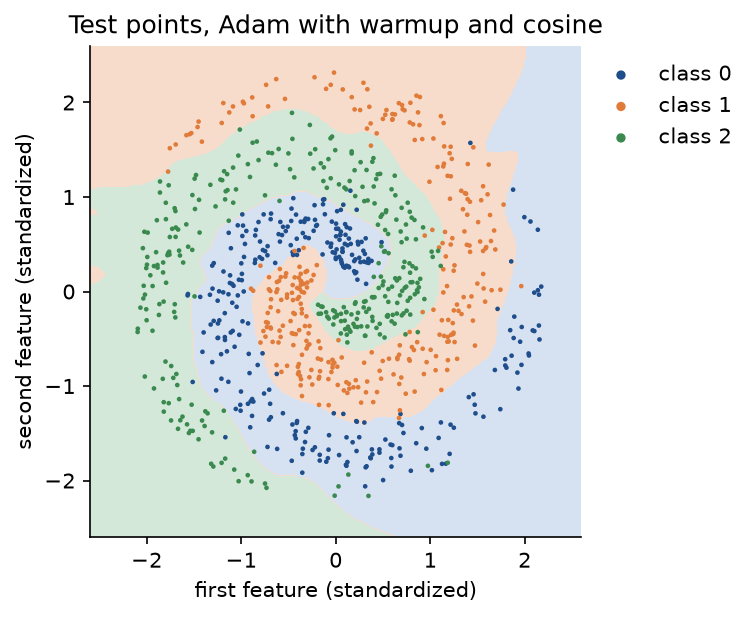
The regions follow the spiral arms through more than a full turn, and the errors sit where the noise makes neighbouring arms overlap, which is why no configuration passes about 95 % test accuracy.

Last, the batch-size study. The per-example gradients at the initial weights confirm the noise formula: for a batch of 32 it predicts an expected squared error of 0.31363, and 2000 random batches give 0.31189; for eight examples and batches of three, enumerating all 56 batches gives 2.6347353771, the formula's value to every printed digit. The noise scale is 8.8 at the start, 10.4 after 5 epochs of momentum training, 73.6 after 20 and 157.2 after 60: as the true gradient shrinks, ever larger batches are needed before the noise stops dominating. Momentum is then trained at four batch sizes for the same 60 epochs, with the best of three learning rates around the linear-scaling guess 0.1 m / 32, judged by the mean cost over the last 10 epochs:

• m = 8: guess 0.025, best 0.0125, 6780 steps, mean cost 0.1660.
• m = 32: guess 0.1, best 0.1, 1740 steps, mean cost 0.1646.
• m = 128: guess 0.4, best 0.1, 480 steps, mean cost 0.3081.
• m = 900, the whole training set: guess 2.8125, best 1.4062, 60 steps, mean cost 0.1457.

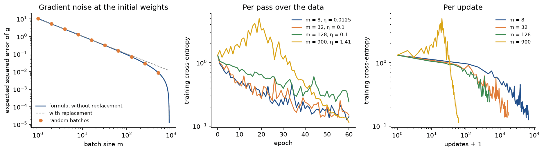
Per update, larger batches make far more progress: the full batch reaches a cost comparable to m = 32 in 60 updates instead of 1740. Per pass over the data the small batches are ahead early. The guess is exact for m = 32 by construction; for m = 8 and m = 900 the best rate was half of it, and for m = 128 a quarter. In practice the rule is a starting point for a learning rate that is then tuned, and it breaks down where the stability limit of the curvature, not the noise, sets the largest usable step.

Some of these runs sit near the edge of stability, where rounding differences of 10⁻¹⁶ grow exponentially (see In practice). The individual costs of those runs, Adam at its best constant rate in particular, can come out noticeably differently on another CPU or linear algebra library, while the conclusions above do not change.

The notebook optimizers.ipynb follows this page: the worked example and Adam in bare NumPy, momentum on an ill-conditioned quadratic, bias correction, the trajectories, the schedules, weight decay, clipping, the pitfalls below, the benchmark on three spirals and finally the comparison with PyTorch, with every plot drawn inline. It runs in under a minute on one CPU thread. The tests in tests check the worked example value by value, the analysis of every section, the key numbers of the experiments on test surfaces and the agreement with PyTorch, and run in about five seconds:

python -m pytest neural-networks/optimizers

The three spirals are synthetic, generated by spirals from a seed, so nothing is downloaded and no licence is involved.

In practice

torch.optim and torch.optim.lr_scheduler implement the same updates. The spiral network trained the usual PyTorch way looks like this, here with AdamW, a one-cycle schedule and clipping:

import torch

from optimizers import batches, initialize_network, spiral_problem, to_torch_network

problem = spiral_problem()
model = to_torch_network(initialize_network([2, 32, 32, 3], seed=0))
features = torch.from_numpy(problem.train_inputs)
targets = torch.from_numpy(problem.train_labels)
optimizer = torch.optim.AdamW(model.parameters(), lr=0.03, weight_decay=0.01)
scheduler = torch.optim.lr_scheduler.OneCycleLR(optimizer, max_lr=0.05, total_steps=1740)
for batch in batches(900, 60, 32):
    index = torch.from_numpy(batch)
    optimizer.zero_grad()
    torch.nn.CrossEntropyLoss()(model(features[index]), targets[index]).backward()
    torch.nn.utils.clip_grad_norm_(model.parameters(), 1.0)
    optimizer.step()
    scheduler.step()

examples/compare_with_pytorch.py checks the agreement at three levels. On the worked example the two implementations agree to within 2.2 × 10⁻¹⁶. On 300 steps of mini-batch gradients of the spiral network, recorded along our run and replayed to PyTorch so that only the update rules are compared, the largest parameter difference is at most 8.9 × 10⁻¹⁶ for every configuration: SGD plain, with momentum, with Nesterov momentum and with dampening and L2 decay; Adagrad plain and with learning-rate decay, weight decay and an initial accumulator; RMSprop plain and centered with momentum and weight decay; Adam, Adam with L2 and AdamW. Each of the five schedules, driving momentum SGD and Adam with clipping at norm 1, agrees to 6.9 × 10⁻¹⁷ in the learning rate, exactly in the cycled momentum and to 1.3 × 10⁻¹⁵ in the parameters. The tests repeat these checks on random parameters and gradients with tolerances of 10⁻¹³ (test_matches_torch_optim_on_identical_gradients, test_scheduled_and_clipped_runs_match_pytorch) and along trajectories where each side computes its own gradients, to 10⁻¹² (test_matches_torch_optim_along_a_trajectory).

Training the project's twelve configurations the usual PyTorch way, with autograd, CrossEntropyLoss, torch.optim and the schedulers, from the same weights and batches, the loss curves agree to within 4.5 × 10⁻¹³ after the first epoch. After 60 epochs seven configurations still agree to within 2.7 × 10⁻¹³, while momentum, AdaGrad, Adam, AdamW and Adam with one-cycle differ by 1.2 × 10⁻³, 5.8 × 10⁻⁸, 4.3 × 10⁻², 6.4 × 10⁻⁷ and 2.8 × 10⁻⁶. That is not a disagreement but chaos: adding 10⁻¹⁵ to every initial weight of our own NumPy run moves its loss curve by even more, 3.2 × 10⁻³, 6.0 × 10⁻⁷, 6.9 × 10⁻², 1.0 × 10⁻⁵ and 2.7 × 10⁻⁵. At learning rates near the edge of stability, rounding differences of 10⁻¹⁶ grow exponentially, so two implementations can only be compared step by step on the same gradients, never by running both to the end and comparing the results.

When to use which:

• Adam or AdamW with a warmup and a decaying schedule is the robust default for most networks, and the standard for transformers, as in A tiny GPT; use AdamW rather than Adam with weight_decay whenever weight decay is wanted.
• SGD with momentum 0.9 (Nesterov or not) and a step, cosine or one-cycle schedule remains competitive for convolutional networks and is the method most analyses assume; it needs a more carefully tuned learning rate.
• RMSProp is common in reinforcement learning and recurrent networks; AdaGrad suits convex problems with sparse features and short runs.
• Whatever the optimizer, tune the learning rate first, on a logarithmic grid or with a range test, and judge by the final cost, on more than one seed.
• Clip the global gradient norm for recurrent networks and whenever loss spikes appear; set the threshold from the typical norms of a healthy run.
• Use the from-scratch versions to learn the updates, to reason about a run that misbehaves and to read papers; use torch.optim for anything else. For a new optimizer, check the code against a framework on a few steps with identical gradients, as above, rather than comparing end results.

Pitfalls

• Comparing optimizers at one learning rate, or untuned. The best rates in the spiral sweep span a factor of 30, from 0.01 for RMSProp to 0.3 for SGD. At a shared rate of 0.01 RMSProp looks best (0.1047) and SGD worst (0.8589); at 0.3 SGD is second best and RMSProp the worst of all (7.7237). Compare each optimizer at its own tuned rate, and on several seeds, as project/optimizer_benchmark.py does.
• Expecting adaptive methods to fix any ill-conditioning. AdaGrad, RMSProp and Adam rescale coordinates, which helps only when the steep and flat directions are aligned with the axes. Rotating the quadratic by 45 degrees leaves gradient descent and momentum unchanged but raises AdaGrad's cost after 80 steps from 1.84 × 10⁻¹¹ to 7.24 × 10⁻³ (examples/trajectories.py, test_rotation_leaves_gradient_descent_unchanged_but_not_adagrad).
• Ignoring the start-up of RMSProp and uncorrected Adam. RMSProp has no bias correction, so its first step is η divided by the root of 1 - ρ in every coordinate: 1.0 instead of 0.1 for ρ = 0.99 on the worked example, and 3.1623 for ρ = 0.999 (examples/adaptive_steps.py). An Adam written without bias correction takes steps up to 6.5685 times too long for hundreds of steps. Use warmup with RMSProp, and keep the correction in Adam.
• Using Adam's weight_decay as if it were weight decay. torch.optim.Adam(weight_decay=...) adds an L2 term to the gradient, which Adam then normalizes: an idle weight decays at the same speed for λ = 0.1 and 0.5, and noisy weights barely decay at all (examples/adaptive_steps.py). Use AdamW, and do not copy a weight_decay value between the two or between frameworks: PyTorch's AdamW decays by lr * weight_decay per step.
• Stepping the schedule wrongly. A cosine schedule run past its period climbs back to its starting value: k = 100, 150 and 200 give 0, 0.05 and 0.1 for a period of 100. A period given in epochs but stepped every mini-batch makes the 60-epoch schedule pass through 14 minima in 1740 steps. Calling scheduler.step() before optimizer.step() skips the first value, so the rates used become 0.05, 0.025 and 0.0125 instead of 0.1, 0.05 and 0.025, and PyTorch warns about it (examples/schedules_and_clipping.py and examples/compare_with_pytorch.py). OneCycleLR raises an error when stepped more than total_steps times, and OneCycle here does the same.
• Porting momentum hyperparameters between conventions. PyTorch's form, v = βv + g, reaches steps of η / (1 - β), the exponential-average form only η, a factor of 10 at β = 0.9. The classical form, which stores the step itself as u = βu - ηg, matches PyTorch for a constant rate but not when the rate changes: after a drop from 0.1 to 0.01 with a constant gradient, PyTorch's step falls at once from 0.9982 to 0.0998, while the classical one decays over a few tens of steps, still 0.4132 at step 70 and 0.2092 at step 80 (examples/schedules_and_clipping.py).
• Forgetting to zero the gradients. PyTorch accumulates into .grad. Without optimizer.zero_grad() each step uses the sum of all gradients so far, which acts like momentum with β = 1: on the worked quadratic the cost after 50 steps is 0.6614 instead of 0.0530, and it never settles (examples/compare_with_pytorch.py).
• Treating clipping as a cure for a large learning rate. Clipping bounds each step but does not make a rate above the local stability limit converge: on the recurrent unit the clipped run bounces for ever at a cost of 1.21. Combine clipping with a decaying rate, and compute the global norm over all parameters, since clipping each tensor separately changes the direction of the update.
• Judging an optimizer by its early progress or by one run. After 10 epochs the adaptive methods lead the SGD family by a wide margin; after 60 the order is different and the schedules dominate. The worst of three seeds for Adam at its sweep-best rate is 43 % above its median. Report final costs over several seeds.
• Comparing implementations end to end. Rounding differences of 10⁻¹⁶ grow exponentially at learning rates near the edge of stability: an Adam run nudged by 10⁻¹⁵ ends with a loss about 0.07 away from the original. Agreement between two implementations is tested step by step on identical gradients.
• Summing instead of averaging the batch gradient. The update then scales with the batch size, which silently multiplies the learning rate by m; see Backpropagation for the gradient check that catches it.

Further reading

• H. Robbins and S. Monro, "A stochastic approximation method", Annals of Mathematical Statistics 22(3), 400-407, 1951.
• B. T. Polyak, "Some methods of speeding up the convergence of iteration methods", USSR Computational Mathematics and Mathematical Physics 4(5), 1-17, 1964. The heavy-ball method and its rate on quadratics.
• Y. Nesterov, "A method for solving the convex programming problem with convergence rate O(1/k²)", Soviet Mathematics Doklady 27, 372-376, 1983.
• I. Sutskever, J. Martens, G. Dahl and G. Hinton, "On the importance of initialization and momentum in deep learning", ICML 2013. The look-ahead form of Nesterov momentum used by deep-learning libraries.
• J. Duchi, E. Hazan and Y. Singer, "Adaptive subgradient methods for online learning and stochastic optimization", Journal of Machine Learning Research 12, 2121-2159, 2011. AdaGrad.
• D. P. Kingma and J. Ba, "Adam: a method for stochastic optimization", ICLR 2015, arXiv:1412.6980.
• S. J. Reddi, S. Kale and S. Kumar, "On the convergence of Adam and beyond", ICLR 2018. AMSGrad.
• I. Loshchilov and F. Hutter, "Decoupled weight decay regularization", ICLR 2019, arXiv:1711.05101. AdamW.
• I. Loshchilov and F. Hutter, "SGDR: stochastic gradient descent with warm restarts", ICLR 2017. Cosine annealing.
• L. N. Smith, "Cyclical learning rates for training neural networks", WACV 2017. The learning-rate range test.
• L. N. Smith and N. Topin, "Super-convergence: very fast training of neural networks using large learning rates", 2019, arXiv:1708.07120. The one-cycle policy.
• P. Goyal et al., "Accurate, large minibatch SGD: training ImageNet in 1 hour", arXiv:1706.02677, 2017. Linear scaling and warmup.
• S. McCandlish, J. Kaplan, D. Amodei and the OpenAI Dota team, "An empirical model of large-batch training", arXiv:1812.06162, 2018. The gradient noise scale.
• L. Liu et al., "On the variance of the adaptive learning rate and beyond", ICLR 2020. Why Adam needs warmup.
• R. Pascanu, T. Mikolov and Y. Bengio, "On the difficulty of training recurrent neural networks", ICML 2013. Exploding gradients, cliffs and clipping.
• Y. Dauphin et al., "Identifying and attacking the saddle point problem in high-dimensional non-convex optimization", NeurIPS 2014.
• L. Lessard, B. Recht and A. Packard, "Analysis and design of optimization algorithms via integral quadratic constraints", SIAM Journal on Optimization 26(1), 57-95, 2016. A strongly convex function on which the tuned heavy ball fails.
• L. Bottou, F. E. Curtis and J. Nocedal, "Optimization methods for large-scale machine learning", SIAM Review 60(2), 223-311, 2018.
• R. M. Schmidt, F. Schneider and P. Hennig, "Descending through a crowded valley: benchmarking deep learning optimizers", ICML 2021. Why fair optimizer comparisons need tuning budgets and several seeds.
• G. Goh, "Why momentum really works", Distill, 2017.
• I. Goodfellow, Y. Bengio and A. Courville, Deep Learning, chapter 8, MIT Press, 2016.