Decoding strategies

A language model never writes text. At every step it returns a probability for each token in its vocabulary, and something else has to turn that sequence of distributions into one output. That something is the decoding strategy, and it matters as much as the model: the same network can produce endless loops, one safe sentence, word salad or valid JSON depending on how its scores are used. This page treats every common strategy against one interface, a function from a token prefix to next-token log-probabilities: greedy decoding, beam search with length normalization, temperature, top-k, top-p and min-p sampling, repetition and frequency penalties, decoding constrained by a regular expression, and self-consistency. Each one is derived, worked through on distributions small enough to check by hand, implemented in NumPy and finally run on a character-level model trained on a public-domain novel. Afterwards you will be able to predict what a decoding setting will do before you run it, explain the classic failures (repetition, empty outputs, nonsense, broken formats) from the mathematics, and measure the trade-off between quality and diversity instead of guessing. It builds on A tiny GPT, whose model any of these strategies can decode.

To run the code in this topic, install the base group, and the deep group for training the character model, the sample project, the notebook and the comparisons with PyTorch.

Intuition

Every possible output is a path through a tree. The root is the prompt, each node has one child per vocabulary token, and the probability of a path is the product of the probabilities along it. With a vocabulary of |V| tokens there are |V|ⁿ paths of length n, far too many to score, so every strategy is a rule for walking down the tree without looking at all of it.

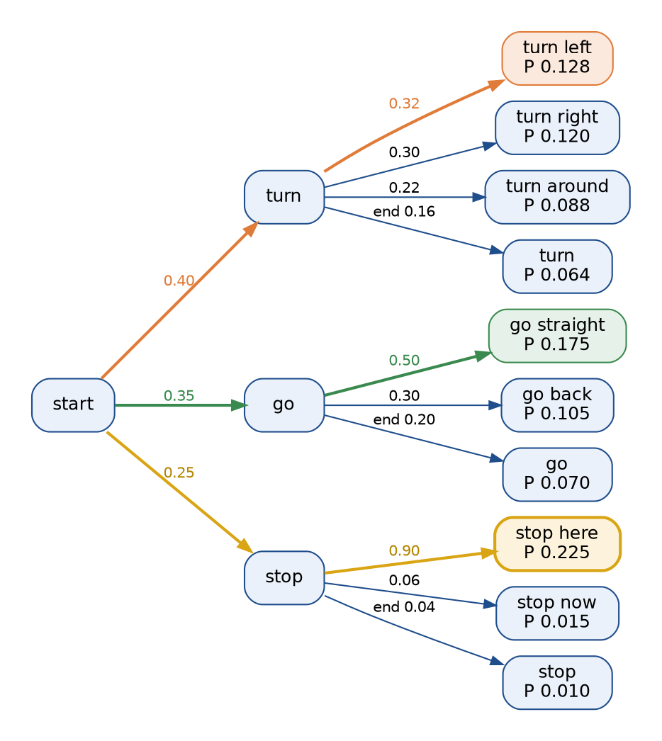
The tree is the small command model of the worked example. Greedy decoding follows the orange path, always taking the most probable child, and ends with probability 0.128. A beam that keeps two prefixes finds the green path, 0.175, and the most probable command of all, in amber, starts with the least probable first word. There are two families of strategies:

• Search tries to find a path of high probability. Greedy decoding takes the best child at every node. Beam search keeps the k best partial paths at each depth. Both are deterministic, and both inherit whatever the model's most probable outputs are like, which for open-ended text is often short or repetitive.
• Sampling draws a random path, choosing each token in proportion to its probability. Pure sampling reproduces the model's distribution, including its long tail of unlikely tokens, which is where nonsense comes from. Temperature reshapes the distribution, and top-k, top-p and min-p cut the tail off before drawing.

Penalties and constraints sit in between: they edit the scores at each step before either family uses them, to discourage repetition or to forbid tokens that would break a required format. Self-consistency works one level up. It samples several complete answers and returns the most common final result, which estimates the most probable answer rather than the answer of the most probable path.

Every strategy on this page is one pass around this loop per token. The model is called once, a fixed list of processors edits its scores, and a chooser picks the next token, so changing the strategy never means changing the model. In short:

• Greedy decoding takes the most probable token at each step. It is deterministic and suits short, closed answers or a baseline.
• Beam search keeps the k most probable prefixes. It is deterministic and is the usual choice for translation, speech recognition and summarization.
• Temperature divides the logits by T before the softmax. It is the main dial between safe and varied text.
• Top-k samples from the k most probable tokens, a fixed cut of the tail.
• Top-p, or nucleus sampling, samples from the smallest set of tokens with mass at least p, a cut that adapts to the distribution.
• Min-p samples from the tokens at least p_min times as probable as the best one, an adaptive cut that tolerates high temperatures.
• Repetition penalties lower the scores of tokens already used, for open-ended generation.
• Constrained decoding forbids tokens that would break a grammar, for JSON, code and other fixed formats.
• Self-consistency votes over several sampled answers, for questions with one checkable final answer.

How it works

Notation

Tokens are numbered 0 to |V| - 1, where V is the vocabulary and |V| its size. The prompt is x and the generated tokens are y1 to yn; y<t stands for the tokens before step t. One token, the end token <eos>, finishes an output, and the length |Y| of an output counts it. At step t the model gives logits zt, one per token, and the next-token probability p(v | x, y<t) is their softmax. The next-token log-probability is ℓt(v), always with the natural logarithm, so entropies are in nats. The beam width is k, the temperature T, the length-penalty exponent α and its base b. The formula images write indices as subscripts, as in z with subscript t; the text writes them plainly, as zt or ℓt.

The decoding interface

An autoregressive model factorizes the probability of an output into next-token probabilities, so the log-probability of an output is a sum:

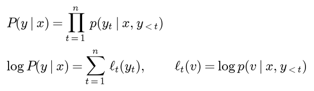
Everything a decoder needs is therefore one function, from (x, y<t) to the vector ℓt of next-token log-probabilities. Any model that provides it, an n-gram table, a recurrent network, a transformer or a hand-written tree, can be decoded by the same code, and every strategy on this page is defined only in terms of that vector. Strategies that edit scores are written as processors: functions of the prompt, the tokens generated so far and the current score vector that return a new score vector, applied in a fixed order before a token is chosen.

Because the softmax ignores a constant added to every logit, logits and log-probabilities, which differ by the logarithm of the normalizing sum, define the same distribution. A processor that is not shift-invariant in the same way gives different results on the two, which matters for the repetition penalty below.

Greedy decoding

Greedy decoding chooses the most probable token at every step and stops at the end token or a length limit:

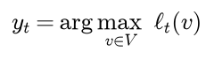
It costs one model call per token. It does not find the most probable sequence: it maximizes each factor of the product separately, and a slightly less likely first token can lead to continuations that are far more likely. The worked example builds such a case.

Beam search

Beam search keeps up to k live hypotheses, prefixes that have not ended, scored by their summed log-probability:

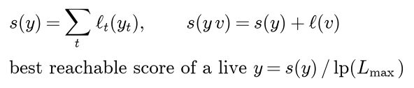
One step runs as follows:

1. Extend every live hypothesis by every token, giving up to k|V| candidates, each scored by its parent's score plus the token's log-probability.
2. Sort the candidates by score and walk down the list. A candidate that ends with the end token joins the finished list if its rank is below k; any other candidate joins the new beam; stop once the new beam holds k hypotheses.
3. If no live hypothesis remains, or the length limit is reached, stop. Hypotheses still live at the length limit join the finished list, marked as unfinished.

The answer is the finished hypothesis with the best final score. Each step costs k model calls and a sort of k|V| numbers, so n steps cost on the order of nk|V| score evaluations. With k = 1 and no length normalization it reproduces greedy decoding. With k at least the number of candidates at every step, nothing is pruned and the search is exhaustive.

It can also stop early. Every log-probability is at most zero, so a live hypothesis's score can only fall as it grows. When at least k hypotheses have finished and the k-th best of them already beats the best score any live hypothesis could still reach, more steps cannot change the top k. For the normalized score below, that best reachable value is the second line of the formula above: the current score, which can only decrease, divided by the length penalty at the length limit, which can only grow.

Length normalization

Every extra token multiplies the probability by a number below one, so the raw score favours short outputs. In the extreme, a model that gives the end token probability 0.4 at the start makes the empty output more probable than any sentence whose probability is below 0.4, and exact search returns nothing. The usual remedy divides the score by a length penalty:

With b = 5 this is the penalty introduced for Google's neural machine translation system (GNMT). With b = 0 it is the length to the power α, the form most libraries use, and α = 1 then gives the mean log-probability per token. α = 0 switches normalization off, larger α favours longer outputs, and the penalty always equals 1 for a single token. The implementation, like common libraries, ranks live hypotheses by the raw score during the search and applies the penalty to finished ones.

Normalization swaps one degenerate optimum for another. Suppose a model can repeat a cycle of m tokens with probability q per cycle, and the rest of an output, the part that does not repeat, has c′ tokens and log-probability c. An output with r cycles then has a mean log-probability per token of

When δ is negative, which says that the part that does not repeat is worse per token than the cycle, the second term shrinks towards zero as r grows. The per-token score then rises with every repetition towards ln(q) / m, and the best output is as long as the length limit allows. In the chorus example below, m = 3, q = 0.4, c′ = 0 and δ = 2 ln 0.6 - ln 0.4 = -0.1054.

Temperature and entropy

Temperature T > 0 rescales the logits before the softmax:

As T goes to 0 the distribution concentrates on the largest logit, and sampling becomes greedy decoding; at T = 1 it is the model's distribution; as T grows without bound it becomes uniform over the tokens with finite logits. Dividing all logits by the same positive number never changes which one is largest, so temperature has no effect on greedy decoding or on the ranking used by top-k.

The entropy measures how spread out a distribution is, zero for a certain outcome and ln |V| for a uniform one:

It rises monotonically with temperature, and the rate has a closed form. Write β = 1/T and let Z be the normalizing sum. The entropy is then ln Z minus β times the mean logit, the derivative of ln Z with respect to β is the mean logit, and the derivative of the mean logit is the variance of the logits, all under the tempered distribution:

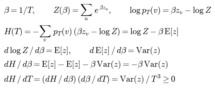
The derivative is zero only when all logits with non-zero probability are equal. The entropy starts at ln g for g tied largest logits (zero for a unique maximum) and rises to ln |V|. The rate is largest where the distribution has the most spread in logit space, which is why a small change of temperature can change the character of the text abruptly. Entropy itself is treated in information theory.

Truncation: top-k, top-p and min-p

Each rule keeps a set K of tokens and samples from the distribution renormalized over it:

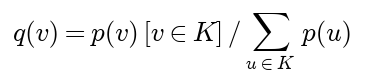
Rank the probabilities in decreasing order, with ties broken by the lower token id, and let Mi be the mass ranked strictly above position i. The three rules keep:

• Top-k keeps the first k positions.
• Top-p keeps the smallest prefix whose mass reaches p. The first token always survives because nothing is ranked above it, and the last kept token is the one that carries the cumulative mass to p or beyond.
• Min-p keeps every token at least p_min times as probable as the most probable one. The threshold scales with the model's confidence: a peaked distribution keeps few tokens, a flat one many.

Top-k ignores the shape of the distribution: k = 10 is too many after "the capital of France is" and too few after "my favourite word is". Top-p and min-p adapt. Because both are defined on probabilities, they interact with temperature: applied after a temperature above 1, they keep more tokens than before it. This package applies processors in the order given; libraries generally apply temperature first, but check.

Repetition and frequency penalties

Let cv count how often token v already occurs in the text. Three families of penalty are common.

The CTRL repetition penalty with θ > 1 edits the score of every token seen at least once:

Both branches make the score smaller, but which one applies depends on the sign of the score, and an added constant can flip the sign. The rule is therefore not shift-invariant: two logit vectors that define the same distribution can give different penalized distributions. Applied to log-probabilities, which are never positive, it always multiplies, and so raises the probability of every seen token to the power θ before renormalization:

Frequency and presence penalties subtract a charge per occurrence and a flat charge for having appeared at all:

Subtraction commutes with adding a constant, so these are shift-invariant. The third family, n-gram blocking, sets the score of any token that would complete an n-gram already present in the text to minus infinity. It removes exact repetition and nothing else.

All three act on tokens, so their meaning depends on what a token is. With word or subword tokens, "the" and "witch" are penalized as units; with characters, every common letter has been seen after a few words, and the penalty no longer targets repetition at all.

Constrained decoding

A format, such as "a JSON object with these keys", defines a set L of valid strings. Constrained decoding computes, at each step, the set A(y<t) of tokens after which the output can still be completed into a member of L, and masks the rest:

For a regular language, A comes from a finite automaton. compile_regex parses a pattern with groups, alternation, character classes and the quantifiers *, +, ? and {m,n}, and builds a nondeterministic automaton by Thompson's construction: one small fragment per syntax element, joined by transitions that read no input. The decoder tracks the set S of automaton states reachable after the generated text. A token is allowed when reading its characters from S leaves a non-empty set, and the end token is allowed when S contains the accepting state.

Masking alone does not guarantee a valid output under a length limit: a pattern such as [a-z]+\} can keep the model writing letters until the budget runs out. The fix is a distance table. For every automaton state s, a breadth-first search backwards from the accepting state, with cost 1 for transitions that read a character and 0 for the others, gives d(s), the fewest characters still needed. With B tokens of budget left, a token is allowed only if the state set S′ after it leaves room for the remaining characters plus the end token:

For character tokens this is exact, and every output is then valid and complete within the limit.

The diagram shows these distances for the pattern of the worked example, with the automaton simplified to the states a decoder actually visits. At the amber state both branches are possible, but false needs one character more than true, so a budget that is one token short removes the f branch alone.

Masking is not the same as conditioning on validity. The model's distribution given that the output is valid is p(y) restricted to L and renormalized by P(L). Masking and renormalizing at every step gives instead a distribution q that divides by a different normalizer Z at every step:

The product of the Z values differs between outputs: a prefix after which the model puts little mass on allowed tokens has a small Z and gets boosted. Exact conditioning would need, at each step, the probability of eventually completing a valid string, which is generally intractable. Beam search over masked but unrenormalized scores ranks complete outputs by p(y) itself and so finds the most probable valid output among those it keeps.

Self-consistency

For tasks with a checkable final answer, let a(y) extract the answer from an output, for example the last number. Different outputs, different reasoning paths, can reach the same answer, so the answer has the marginal distribution

Greedy decoding and beam search approximate the most probable output and report its answer. Self-consistency samples N outputs, extracts their answers and returns the most frequent one, which estimates the most probable answer. The two differ whenever the correct answer's probability is spread over many paths while a wrong answer comes from one concentrated path.

If the answers have probabilities π1 to πA, the vote counts n1 to nA are multinomial, and the probability that the correct answer a* wins is a sum over every table of counts:

The weight w shares a tie equally among the tied answers. As N grows this tends to 1 if a* is the unique most probable answer and to 0 if another answer is. Voting cannot fix systematic errors; it only removes scattered ones. Temperature controls the trade-off: as T goes to 0 every sample is the greedy path and voting adds nothing, while a very high temperature makes every answer more equal and requires more samples to separate them.

Measuring diversity and quality

• Entropy of the distribution that was actually sampled, averaged over steps: how much randomness a strategy injected. Zero for greedy decoding and beam search.
• Entropy of the model's own distribution along an output: how confident the model was on that path. Repetition loops show up as stretches of low entropy.
• Distinct-n: the number of distinct n-grams divided by the total number of n-grams over a set of outputs. It falls with repetition within and across outputs. It also depends on how much text is pooled, so compare sets of the same size.
• Repeated n-gram fraction within one output: one minus distinct over total for that output alone.
• Sequence log-probability, or its value per token, whose negative exponential is the perplexity. It is what search maximizes, which makes it a poor judge of search: the model's own favourite text is often its most repetitive.
• An external check the model does not optimize, here the share of generated words that occur in the training text. For real systems, human ratings or a separate judging model play this role.

A perplexity of P means the model was, on average, as uncertain as a uniform choice among P tokens, so lower is better for the model and says nothing yet about whether the text is good.

Worked example

All logarithms are natural and every value is computed at full precision, then rounded to four decimals. When a sum written out from rounded terms differs from the full-precision value in the last digit, the text says so. Every number in this section is asserted by tests/test_worked_examples.py and tests/test_voting.py, and printed by the example scripts named in each subsection.

Greedy decoding versus beam search

A model of spoken commands has eleven tokens. Its first word and the word that follows have these probabilities, and every two-word command ends with <eos> for certain:

• At the start: turn 0.40, go 0.35, stop 0.25.
• After turn: left 0.32, right 0.30, around 0.22, <eos> 0.16.
• After go: straight 0.50, back 0.30, <eos> 0.20.
• After stop: here 0.90, now 0.06, <eos> 0.04.

The log-probabilities needed are ln 0.40 = -0.9163, ln 0.35 = -1.0498, ln 0.25 = -1.3863, ln 0.32 = -1.1394, ln 0.30 = -1.2040, ln 0.22 = -1.5141, ln 0.16 = -1.8326, ln 0.50 = -0.6931, ln 0.20 = -1.6094 and ln 0.90 = -0.1054.

Greedy decoding picks turn (0.40), then left (0.32), then <eos>, for log P = -0.9163 - 1.1394 + 0 = -2.0557 and P = 0.40 × 0.32 = 0.128.

Beam search with k = 2. Step 1 scores the three first words, -0.9163, -1.0498 and -1.3863, and keeps turn and go. Step 2 extends both by every token with non-zero probability, which gives seven candidates in this order:

1. go straight, -1.0498 - 0.6931 = -1.7430, kept.
2. turn left, -0.9163 - 1.1394 = -2.0557, kept.
3. turn right, -0.9163 - 1.2040 = -2.1203.
4. go back, -1.0498 - 1.2040 = -2.2538.
5. turn around, -0.9163 - 1.5141 = -2.4304.
6. go <eos>, -1.0498 - 1.6094 = -2.6593.
7. turn <eos>, -0.9163 - 1.8326 = -2.7489.

Two of these sums written out from rounded terms, -1.7429 and -2.6592, differ in the last digit from the full-precision values shown.

Neither end-token candidate ranks in the top two, so nothing finishes yet. Step 3 adds <eos> with log-probability 0 to both beams, both finish, and the search returns go straight with probability 0.35 × 0.50 = 0.175. Beam search beats greedy decoding because go is only slightly less likely than turn, while its best continuation is far more likely.

With k = 3 the beam also keeps stop after step 1, the least likely first word, and stop here scores -1.3863 - 0.1054 = -1.4917, probability 0.25 × 0.90 = 0.225. Enumerating all ten complete commands confirms that this is the most probable output. The best sequence starts with the worst first word, which no amount of step-by-step greed would find. examples/greedy_and_beam.py prints the whole trace.

Length normalization and the chorus model

The chorus model is a Markov chain over <eos>, we, sing and and. At the start it says we with probability 0.6 and ends at once with probability 0.4. After we comes sing; after sing it ends with probability 0.6 or says and; after and comes we. Every complete output is the chorus "we sing" repeated r times, with log-probability 2 ln 0.6 + (r - 1) ln 0.4 and length 3r counting the end token. With ln 0.6 = -0.5108 and ln 0.4 = -0.9163, the outputs up to twelve tokens score as follows, giving the length, the log-probability, the score per token (b = 0, α = 1) and the GNMT score (b = 5, α = 1):

• The empty output <eos>: length 1, log P -0.9163, per token -0.9163, GNMT -0.9163.
• One chorus, "we sing": length 3, log P -1.0217, per token -0.3406, GNMT -0.7662.
• Two choruses: length 6, log P -1.9379, per token -0.3230, GNMT -1.0571.
• Three choruses: length 9, log P -2.8542, per token -0.3171, GNMT -1.2232.
• Four choruses: length 12, log P -3.7705, per token -0.3142, GNMT -1.3308.

From the rounded logarithms, one chorus scores 2 × (-0.5108) = -1.0216, one unit off in the last digit; building each further row from the row above, -1.0217 - 0.9163 and so on, gives -1.9380, -2.8543 and -3.7706, also one unit off. The GNMT penalties for lengths 1, 3, 6, 9 and 12 are 1, 8/6, 11/6, 14/6 and 17/6.

Greedy decoding says we (0.6 beats 0.4), sing, then <eos> (0.6 beats 0.4): one chorus, probability 0.36. The raw score instead prefers the empty output, 0.40 > 0.36. The per-token score improves with every repetition, since it equals ln(0.4)/3 + (2 ln 0.6 - ln 0.4)/(3r) = -0.3054 - 0.0351/r. Beam search with k = 3 and a limit of twelve tokens returns:

• With the length to the power α: the empty output for α = 0, one chorus for α = 0.5, and four choruses for α = 1 and α = 2.
• With the GNMT penalty: the empty output for α = 0, one chorus for α = 0.5 and α = 1, and four choruses for α = 2.

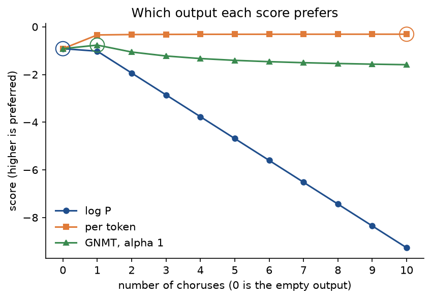
The plot, from examples/greedy_and_beam.py with a limit of 30 tokens, shows the three objectives side by side; the ring on each curve is the output exact search would return. With the per-token score the output grows with the limit, to 30 tokens for a limit of 30 and 60 for 60. More search did not cause either failure; it found what the objective asked for.

Temperature

Six continuations of "the kettle began to", whistle, boil, sing, rattle, hiss and melt, have logits z = (2.0, 1.5, 0.8, 0.2, -0.5, -1.5). The exponentials are (7.3891, 4.4817, 2.2255, 1.2214, 0.6065, 0.2231) with sum Z = 16.1473, so the probabilities at T = 1 are (0.4576, 0.2775, 0.1378, 0.0756, 0.0376, 0.0138).

With ln Z = 2.7818 and a mean logit of 1.4174, the entropy is ln Z minus the mean logit, 1.3643 nats (1.3644 from the rounded terms). Halving and doubling the temperature:

• T = 0.5: probabilities (0.6695, 0.2463, 0.0607, 0.0183, 0.0045, 0.0006), entropy 0.8859 nats.
• T = 1: probabilities (0.4576, 0.2775, 0.1378, 0.0756, 0.0376, 0.0138), entropy 1.3643 nats.
• T = 2: probabilities (0.3130, 0.2438, 0.1718, 0.1273, 0.0897, 0.0544), entropy 1.6473 nats.

The uniform distribution over six tokens has entropy ln 6 = 1.7918. At T = 1 the mean of the squared logits is 2.5866 and the squared mean 2.0090, so the variance of the logits is 0.5776, and the entropy grows at 0.5776 nats per unit of temperature, which a central difference reproduces.

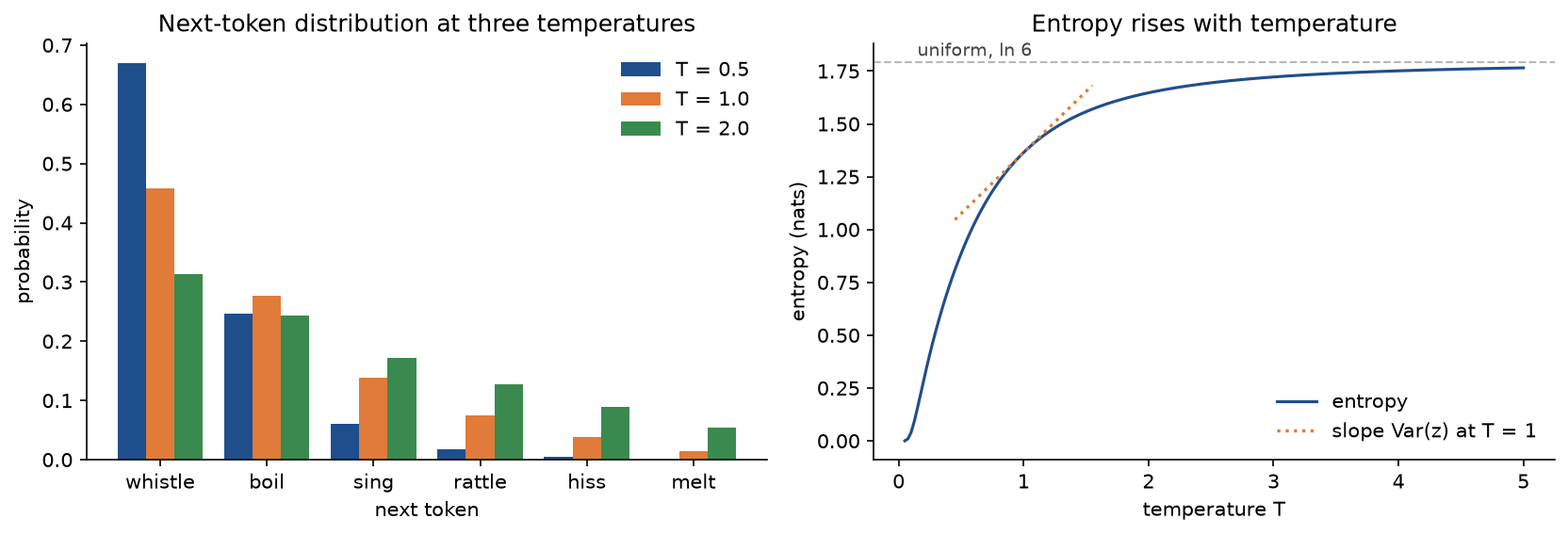
The bars show a higher temperature taking probability from the favourite and handing it down the tail. The tangent at T = 1 has slope 0.5776, the variance of the logits, and the curve is steepest at low temperatures, where a small change of T matters most. examples/temperature_and_truncation.py prints these numbers and draws the figure.

Truncation

On the same distribution at T = 1, the cumulative masses in rank order are 0.4576, 0.7352, 0.8730, 0.9486, 0.9862 and 1.

• Top-k with k = 2 keeps whistle and boil, mass 0.7352, and samples from (0.6225, 0.3775).
• Top-p with p = 0.9: the masses ranked above the six tokens are 0, 0.4576, 0.7352, 0.8730, 0.9486 and 0.9862. The first four are below 0.9, so whistle, boil, sing and rattle are kept, mass 0.9486, and the sampled distribution is (0.4824, 0.2926, 0.1453, 0.0797).
• Min-p with p_min = 0.2 has the threshold 0.2 × 0.4576 = 0.0915 and keeps the three tokens above it, mass 0.8730, distribution (0.5242, 0.3179, 0.1579).

Three rules, three different sets. As the temperature changes, top-k always keeps 2 tokens, top-p keeps 2 at T = 0.5 and 5 at T = 2, and min-p keeps 2 and 5.

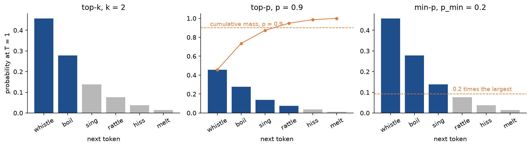
The middle panel shows why top-p keeps rattle: the mass ranked above it is still below 0.9, and it is the token that carries the total past 0.9. The right panel shows the min-p threshold as a fraction of the largest bar, which is why it moves with the model's confidence.

Repetition and frequency penalties

Suppose the text so far contains boil, sing, boil, so boil has been seen twice and sing once.

• CTRL with θ = 1.5 on the logits: both scores are positive, so boil becomes 1.5 / 1.5 = 1.0 and sing becomes 0.8 / 1.5 = 0.5333.
• CTRL with θ = 1.5 on the log-probabilities (-0.7818, -1.2818, -1.9818, -2.5818, -3.2818, -4.2818): both are negative, so boil becomes -1.2818 × 1.5 = -1.9226 and sing becomes -1.9818 × 1.5 = -2.9726 (the products from the rounded terms are -1.9227 and -2.9727).
• CTRL on the logits minus 1, which define the same distribution: boil becomes 0.5 / 1.5 = 0.3333, while sing, now negative, becomes -0.2 × 1.5 = -0.3.
• Frequency 0.5 and presence 0.3: boil becomes 1.5 - 2 × 0.5 - 0.3 = 0.2 and sing becomes 0.8 - 0.5 - 0.3 = 0.0.

The resulting distributions over whistle, boil, sing, rattle, hiss and melt are:

• No penalty: (0.4576, 0.2775, 0.1378, 0.0756, 0.0376, 0.0138).
• CTRL on the logits: (0.5330, 0.1961, 0.1230, 0.0881, 0.0438, 0.0161).
• CTRL on the log-probabilities: (0.5852, 0.1870, 0.0654, 0.0967, 0.0480, 0.0177).
• CTRL on the logits minus 1: (0.4846, 0.2488, 0.1321, 0.0801, 0.0398, 0.0146).
• Frequency 0.5, presence 0.3: (0.6336, 0.1047, 0.0858, 0.1047, 0.0520, 0.0191).

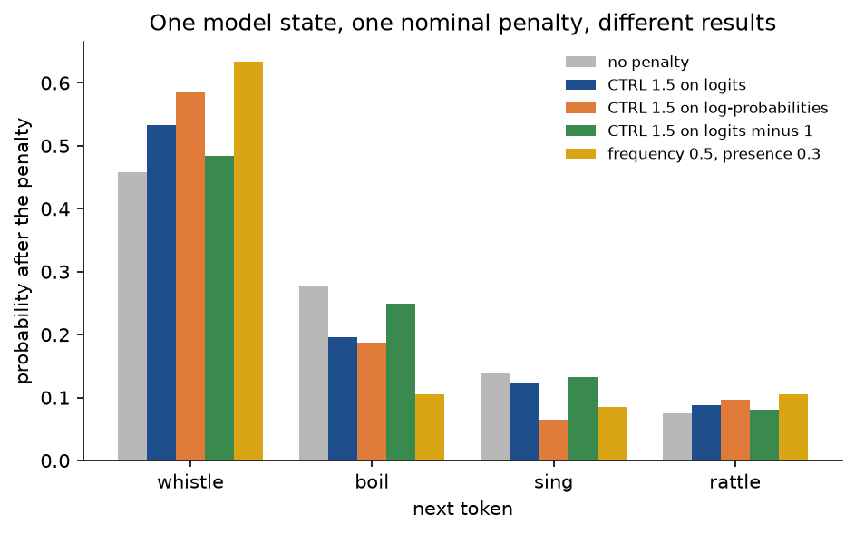
The same model state and the same nominal penalty give boil a probability of 0.1961, 0.1870 or 0.2488 depending on an additive constant the softmax ignores. The frequency penalty gives 0.1047 whatever the constant. examples/repetition_penalties.py prints both lists and draws the figure.

Constrained decoding

The pattern \{"ok": (true|false)\} over a character vocabulary with a separate end token accepts exactly {"ok": true} (12 characters) and {"ok": false} (13). The distance table says that 12 characters are needed from the start, so a budget of at least 13 tokens is required. Walking through {"ok": true}, the mask allows a single character at every step but one: after {"ok": (seven characters), both t and f are allowed if the budget is 14 tokens. There, with 7 tokens left, f leaves alse}, 5 characters plus the end token, which fit in the 6 tokens that remain after it. With a budget of 13, f would need 6 tokens with only 5 left, so only t is allowed: true takes 4 characters plus the end token.

If the model's preferences at that step are " 0.46, t 0.21, 1 0.14, f 0.09 and everything else 0.10, the mask keeps 0.21 + 0.09 = 0.30 of the mass and the decoder samples t with probability 0.21 / 0.30 = 0.7 and f with 0.3; under the tighter budget, t with probability 1. examples/constrained_decoding.py prints the allowed characters at every step under both budgets.

Self-consistency

Four boxes hold 12 pencils each and 3 pencils lie loose. A sampled solution writes a multiplication step, an addition step and <eos>. The first step is 4×12=44 with probability 0.40, 4×12=48 with 0.35 or 12+12+12+12=48 with 0.25. After a correct product the addition gives 51 with probability 0.90 and 52 with 0.10; after the slip it gives 47 with probability 0.95 and 48 with 0.05.

The six complete paths have probabilities 0.3800 (answer 47), 0.3150 and 0.2250 (answer 51), 0.0350 and 0.0250 (answer 52) and 0.0200 (answer 48). The single most probable path is the slip, so greedy decoding and even beam search with k = 3 answer 47. The correct product appears in two equivalent forms, and their paths together give answer 51 a probability of 0.315 + 0.225 = 0.54. The answer distribution is 51 with 0.54, 47 with 0.38, 52 with 0.06 and 48 with 0.02.

A vote over three samples returns 51 when 51 gets at least two votes, probability 3 × 0.54² × 0.46 + 0.54³ = 0.5599, or when all three answers differ and include 51, probability 6 × 0.54 × (0.38 × 0.06 + 0.38 × 0.02 + 0.06 × 0.02) = 0.1024, of which a random tie-break gives 51 one third. In total 0.5599 + 0.0341 = 0.5940. The exact formula gives, for 1, 3, 5, 9, 15 and 25 samples, 0.5400, 0.5940, 0.6403, 0.6923, 0.7424 and 0.7995. A simulation of 2000 votes with N = 5 through self_consistency gives 0.6490, within sampling error of 0.6403. examples/self_consistency.py prints all of these.

The code

The package decoding_strategies is plain NumPy, split into one module per idea. PyTorch is imported only inside the functions of training.py and comparisons.py, so everything else works without it.

• arrays.py holds the types every decoder shares: a model is any function from a tuple of token ids to a score vector, and a processor any function of the prompt, the generated tokens and the scores.
• distributions.py holds the log-space softmax, the entropy, temperature, the stable ranking and keep_only, which removes tokens by setting their score to minus infinity.
• truncation.py holds top_k_filter, top_p_filter and min_p_filter.
• penalties.py holds the CTRL penalty, the frequency and presence penalties and n-gram blocking.
• processors.py wraps them as small frozen objects such as Temperature(0.7) and TopP(0.9), and apply_processors runs a list of them in order.
• models.py holds TableModel and MarkovModel, explicit models for the hand-sized examples, and next_token_log_probabilities, the one call every decoder makes.
• worked_examples.py builds the command, chorus, drink-order, pencil and yes-no models of this page, the kettle logits and the answer pattern, and random trees for the tests.
• decoding.py holds greedy_decode and sample_decode, which share one loop.
• beam_search.py holds beam_search with length normalization, early stopping and an optional trace, and format_beam_trace.
• exhaustive.py enumerates every complete output of a small model, the ground truth for search.
• voting.py holds self_consistency, majority_vote, the exact answer_distribution and majority_vote_accuracy, and the probability of a tie.
• arithmetic.py generates the synthetic arithmetic task and estimates vote accuracy on it.
• regex_syntax.py parses a regular expression into a tree, automaton.py compiles the tree into a Thompson automaton with its distance table, and constraints.py turns it into the RegexConstraint processor.
• metrics.py holds distinct-n, the repeated n-gram fraction, the sequence log-probability and the mean entropy along an output.
• corpus.py downloads, verifies and normalizes the novel, and picks sentence openings as prompts.
• character_model.py holds the character vocabulary and CharacterMLP with its NumPy forward pass, and training.py trains it with PyTorch.
• benchmark.py runs and measures the realistic comparison, and records.py the constrained records.
• comparisons.py writes the model and the truncation rules with PyTorch tensor operations.
• plotting.py and benchmark_plots.py draw every figure in the handbook's four colours.

Greedy decoding and sampling share one loop in decoding.py and differ only in how a token is chosen:

for _ in range(max_new_tokens):
    raw = next_token_log_probabilities(model, prompt + generated)
    token = choose(apply_processors(processors, prompt, generated, raw), rng)
    generated += (token,)
    total += float(raw[token])
    if token in stop:
        return Generation(generated, total, True)

total always adds the model's own log-probability of the chosen token, whatever the processors did, so outputs of different strategies are compared on one scale. The heart of beam search is the walk down the sorted candidates described under How it works, and the heart of the constraint is the budget rule applied to every token:

following = self.transition(states, token)
mask[token] = bool(following) and self.automaton.distance(following) + 1 <= remaining - 1

The examples and the project import the package, so install the repository first as described in the main README. Each example demonstrates one idea and runs in a few seconds from the repository root:

• examples/greedy_and_beam.py prints the greedy result and the full beam trace on the command tree, the drink orders where a wider beam does worse, and the chorus scores under every length penalty, and saves the length-normalization plot.
• examples/temperature_and_truncation.py prints the kettle distribution at three temperatures with its entropy and rate of change, and the tokens each truncation rule keeps, and saves the temperature and truncation figures.
• examples/repetition_penalties.py compares the CTRL rule on logits, log-probabilities and shifted logits with the frequency and presence penalties, shows trigram blocking ending the chorus loop and saves the penalties figure.
• examples/constrained_decoding.py walks through the answer pattern under two budgets, checks the automaton against Python's re module and shows that masking is not conditioning.
• examples/self_consistency.py computes the exact vote accuracy on the pencil question, confirms it by simulation, counts ties and runs the synthetic task, saving its figure.
• examples/compare_with_pytorch.py checks the truncation rules, sampling and the forward pass against PyTorch.

python transformers-and-llms/decoding-strategies/examples/greedy_and_beam.py
python transformers-and-llms/decoding-strategies/examples/temperature_and_truncation.py
python transformers-and-llms/decoding-strategies/examples/repetition_penalties.py
python transformers-and-llms/decoding-strategies/examples/constrained_decoding.py
python transformers-and-llms/decoding-strategies/examples/self_consistency.py
python transformers-and-llms/decoding-strategies/examples/compare_with_pytorch.py

The sample project, project/story_generator.py, is a small story generator built end to end. It downloads the novel, trains the character model on the first nine tenths of it and checks that the NumPy forward pass agrees with PyTorch. Given a prompt, it continues it with the chosen strategy, greedy, beam, sample, temperature, top-k, top-p, min-p or constrained, and reports for every continuation its length, whether it ended a sentence, its log-probability per character, its share of real words and its repeated word triples, and for the set its distinct word pairs. Options such as --temperature, --top-p, --beam-width, --length-alpha, --repetition-penalty, --no-repeat-ngram and --samples change the setting. Without a prompt it runs the comparison described under In practice: every strategy on 40 held-out sentence openings, a temperature sweep and constrained records, and saves three figures; --figures sends them to another folder so a custom run does not overwrite the ones shown here. The default run takes about 40 seconds on one CPU thread and under 1 GB of memory.

python transformers-and-llms/decoding-strategies/project/story_generator.py
python transformers-and-llms/decoding-strategies/project/story_generator.py --prompt "Dorothy was" --strategy top-p --samples 3
python transformers-and-llms/decoding-strategies/project/story_generator.py --prompt "The lion said" --strategy greedy --no-repeat-ngram 12

The model sees only the last twelve characters, so a prompt matters through its end, and in constrained mode only until the first characters of the record have been forced.

The notebook decoding_strategies.ipynb is a guided tour in the order of this page: the command tree, the chorus model, temperature, truncation, penalties, the automaton, the pencil question and the synthetic task, a few pitfalls in code, then the realistic run and the library comparison, with every plot inline. The tests in tests check the worked example value by value, the properties above and the agreement with PyTorch, and run in a few seconds:

python -m pytest transformers-and-llms/decoding-strategies

Data: the realistic run uses The Wonderful Wizard of Oz by L. Frank Baum (1900), Project Gutenberg eBook 55, which is in the public domain in the United States. It is downloaded at runtime into the repository's .data/decoding-strategies/ folder, which git ignores; Project Gutenberg's header, footer and licence text are stripped, and the remaining text is checked against a pinned SHA-256 digest, so a changed edition is reported instead of silently changing the results. All other data is synthetic and generated from fixed seeds.

In practice

Strategies on real text

The project trains a character-level model on the novel: the previous twelve characters, each embedded in 16 dimensions, feed two tanh layers of 384 units and a softmax over 39 characters, in the style of Bengio's neural language model (n-gram language models covers the counting models it improves on). Trained with Adam for 3000 batches of 256 windows, it reaches 1.0637 nats per character on the training text and 1.3802 nats (1.99 bits) on the held-out last tenth, against 3.6636 for a uniform guess. Any autoregressive model fits the same interface, including the transformer of a tiny GPT.

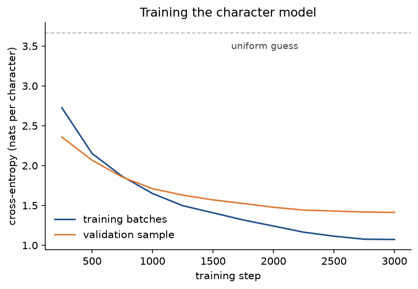
The two curves cross after about 750 steps and then drift apart: the model keeps improving on the text it trains on faster than on the held-out chapters, the usual mild overfitting of a model with about 240 thousand parameters on 186 thousand characters.

Forty sentence openings from the held-out text, such as "dorothy was" and "but the", are continued until a full stop, question mark or exclamation mark, or for at most 150 characters. For each strategy the list gives the mean length in characters, the share of outputs that ended a sentence, the log-probability per character, the share of real words, distinct-2, the share of repeated word triples, and the model's and the sampler's entropy in nats:

• Greedy: 146.5 characters, 0.025 ended, -0.525, 0.983 real words, distinct-2 0.098, 0.252 repeated triples, entropies 1.081 and 0.
• Greedy without repeated 12-grams: 146.5, 0.025, -0.524, 0.986, 0.113, 0.001, 1.042 and 0.
• Beam 5: 16.0, 1.000, -0.564, 1.000, 0.429, 0.000, 0.931 and 0.
• Beam 5 with the per-token score: 149.8, 0.025, -0.310, 0.985, 0.047, 0.685, 0.678 and 0.
• Pure sampling: 63.8, 0.825, -1.407, 0.753, 0.960, 0.000, 1.363 and 1.363.
• Temperature 0.7: 106.2, 0.575, -0.963, 0.883, 0.826, 0.000, 1.245 and 0.887.
• Top-k 10: 74.5, 0.825, -1.251, 0.803, 0.906, 0.000, 1.326 and 1.175.
• Top-p 0.9: 81.7, 0.775, -1.071, 0.844, 0.876, 0.001, 1.272 and 0.981.
• Min-p 0.1: 95.9, 0.600, -0.962, 0.887, 0.852, 0.000, 1.244 and 0.842.
• Temperature 0.7 with CTRL 1.3: 111.9, 0.475, -0.867, 0.929, 0.756, 0.007, 1.223 and 0.729.

The project pins PyTorch and NumPy's linear algebra to one thread and uses deterministic algorithms, so a rerun reproduces every number here. A different thread count changes the trained weights and the forward pass in their last bits, which is enough to send a few sampled outputs down different paths. Typical outputs after "dorothy was":

• Greedy: "strange to see him to see him to see him to see him ..."
• Beam 5: "the wicked witch."
• Beam 5 with the per-token score: "the wicked witch of the wicked witch of the wicked witch of ..."
• Pure sampling: "rept, i will so i portund before."
• Min-p 0.1: "before them the tin woodman for the only and came to help her with the land of oz himself, ..."

Every failure the theory predicts appears. Greedy decoding loops and almost never ends a sentence. Beam search with the raw score ends every sentence after about sixteen characters. With the per-token score it repeats "the wicked witch of" and earns the best model log-probability of all, -0.310 per character, while the model's own entropy along those outputs is the lowest of all: loops are where the model is most sure of itself. Pure sampling is the most diverse and makes up a quarter of its words. Temperature 0.7 and min-p 0.1 give the best balance here. Blocking repeated 12-grams removes exact repetition (0.001) without making greedy text varied (distinct-2 0.113). The CTRL row is the character-level trap described under Pitfalls.

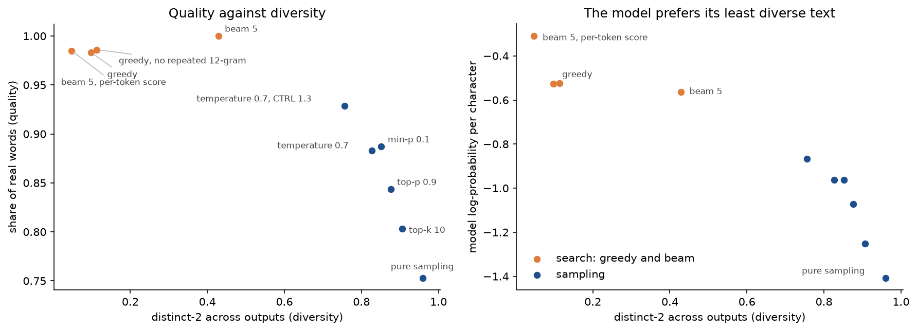
The left panel is the trade-off every strategy chooses a point on: more diversity costs real words. The right panel shows why the model's own score cannot pick the point: it rewards exactly the least diverse, most repetitive text.

A temperature sweep from 0.2 to 1.7 traces the same trade-off continuously: the share of real words falls from 0.971 to 0.315 while distinct-2 rises from 0.315 to 1.000, and repeated word triples, 0.087 at T = 0.2, disappear from T = 0.7 on.

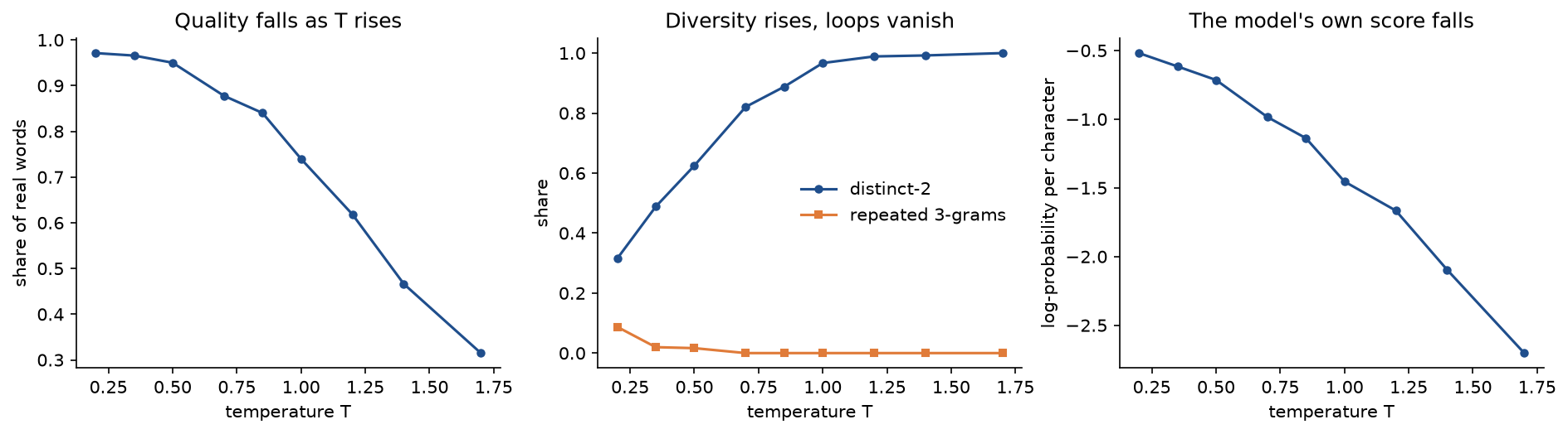
The quality curve stays nearly flat up to T = 0.5 and then falls steadily, while most of the gain in diversity happens below T = 1, which is why moderate temperatures between 0.6 and 0.9 are the common default.

Constrained decoding with the pattern

\{"name": "(dorothy|toto|the scarecrow|the tin woodman|the lion|oz)", "says": "[a-z][a-z ,']{5,40}[.!?]"\}

and a newline as the stop token produced 30 valid records out of 30 sampled at T = 0.8, checked with json.loads, against 0 out of 30 without the constraint; the model has never seen a brace. Greedy decoding under the constraint gives {"name": "dorothy", "says": "i am oz, the scarecrow and the tin woodma!"}. The format is guaranteed and the content is the model's: when the speech reaches the 41-character cap, the mask forces the closing punctuation mid-word. The forced braces and newline cost the model 12.8 nats each on average.

Self-consistency on many problems

examples/self_consistency.py draws 300 synthetic problems of the pencil question's shape, "a groups of b plus c", each with its own probabilities for two correct forms of the product, one or two slips and an addition step. Greedy decoding solves 47.3 %. Voting over 41 samples reaches 73.4 % at T = 1 and 82.6 % at T = 1.5, although a single sample at T = 1.5 is right only 41.0 % of the time; at T = 0.5 voting stalls at 57.6 %. The best temperature grows with the number of samples: 0.5 for one sample (53.2 %), 1.25 for nine (66.4 %) and 2.0 for 41 (84.8 %). The task is built to have the structure self-consistency exploits, so these numbers illustrate the mechanism rather than predict the gain on a real model.

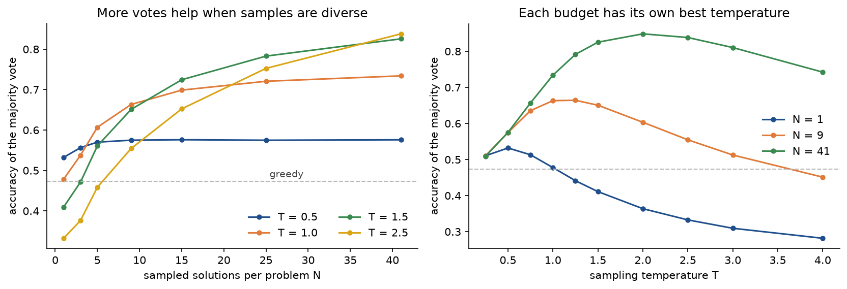
Hotter sampling makes each answer worse but the vote better, because it spreads probability from the single slip towards the two correct forms; the right panel shows that every sampling budget has its own best temperature.

Library equivalents

Hugging Face transformers exposes all of these strategies through generate; it is not a dependency of this topic, so the snippet below is for orientation and was not run here.

from transformers import AutoModelForCausalLM, AutoTokenizer

tokenizer = AutoTokenizer.from_pretrained(name)
model = AutoModelForCausalLM.from_pretrained(name)
inputs = tokenizer("Dorothy was", return_tensors="pt")
sampled = model.generate(**inputs, do_sample=True, temperature=0.7, top_k=0, top_p=0.9)
searched = model.generate(**inputs, num_beams=5, length_penalty=1.0, no_repeat_ngram_size=3)

The package's names map onto the library's arguments as follows:

• greedy_decode is generate with do_sample=False and num_beams=1.
• beam_search(beam_width=k, alpha=a, base=0.0) is num_beams=k, length_penalty=a, which divides the summed log-probability by the length to the power a.
• Temperature(t), TopK(k), TopP(p) and MinP(p) are temperature, top_k, top_p and min_p with do_sample=True. top_k defaults to 50 unless the model's generation config says otherwise, and top_k=0 disables it.
• RepetitionPenalty(theta) is repetition_penalty, the CTRL rule.
• NoRepeatNGram(n) is no_repeat_ngram_size.
• FrequencyPenalty(f, p) is frequency_penalty and presence_penalty in OpenAI-style APIs and vLLM.
• RegexConstraint corresponds to regex and JSON-schema guided decoding in Outlines, XGrammar and vLLM, grammars in llama.cpp and the structured-output modes of hosted APIs.
• self_consistency is num_return_sequences=N with sampling, followed by a vote in your own code.

To check our rules against the way libraries implement them, comparisons.py re-expresses each truncation with PyTorch tensor operations: torch.topk for top-k, an ascending sort, cumulative sum and scatter for top-p (remove a token when the mass at or below it is at most 1 - p, the same rule derived from the other end), and a threshold on the softmax for min-p. On 1000 random logit vectors of 2 to 59 tokens with random parameters the kept sets agree in every case, and tests/test_comparisons.py repeats the check. Sampling 20000 times through torch.multinomial and through our choose_sample gives the same frequencies within two standard errors, and the NumPy forward pass of the trained model agrees with PyTorch's to 1.1 × 10⁻¹⁴ in double precision.

When to use which

• Closed tasks with one right output, such as translation, transcription or extraction: beam search with a modest width (4 to 8) and a length penalty tuned on held-out data, or greedy decoding when latency matters more than the last point of quality.
• Open-ended text: sampling with a temperature around 0.6 to 0.9 and one truncation rule, min-p or top-p. Prefer min-p when you want to raise the temperature for variety; it removes more of the tail as the distribution flattens.
• Repetition in open-ended text: first lower the temperature or try a truncation rule, then add a frequency or presence penalty on word-level tokens, and use n-gram blocking only where exact repeats are always wrong, such as summaries.
• Fixed formats: constrained decoding by masking, with a length budget, rather than validating and retrying. Keep the constrained part small and let the model write free text inside it.
• Questions with a checkable final answer: self-consistency with 5 to 40 samples at a temperature near 1, reporting the vote counts with the answer. Prompting and structured output builds on these, and inference efficiency covers what makes many samples or wide beams affordable.

Pitfalls

• Greedy decoding does not find the most probable sequence. It maximizes each factor separately. On the command tree it returns probability 0.128 while the best sequence has 0.225 and starts with the least likely first word, as examples/greedy_and_beam.py prints.
• A wider beam is not guaranteed to be better. In the drink-order tree, a beam of width 2 keeps both children of coffee at step 2 and prunes tea green, whose continuation is certain: widths 1 and 3 return probability 0.1872, width 2 returns 0.0899 (tests/test_beam_search.py, and the notebook section "A wider beam is not always better"). Beam search is a heuristic; its result is not monotone in the width.
• Exact search can be worse than approximate search. The most probable output of a model is often degenerate. Without normalization the chorus model's best output is empty; with the per-token score it is the longest repetition the limit allows, as the length-normalization plot shows. Translation systems show the same effect: as the beam widens, outputs get shorter and the most probable translation is frequently the empty string. Tune the length penalty on held-out data and do not assume a wider beam helps.
• Using the model's likelihood as a measure of quality. In the realistic run the highest log-probability per character belongs to the "wicked witch of the wicked witch" loop. Judge outputs with something the decoder did not optimize: an external check, a separate model or people.
• Expecting temperature to change greedy decoding. Dividing all logits by T > 0 keeps the largest one largest (tests/test_processors.py). Greedy decoding is the limit of sampling as T goes to 0, and T = 0 itself is not a valid temperature; libraries that accept it switch to greedy decoding.
• The top-p boundary depends on rounding. For the probabilities (0.7, 0.2, 0.1) and p = 0.9 the first two tokens reach 0.9 on paper, but 0.7 + 0.2 = 0.8999999999999999 in double precision, so top-p keeps three tokens, while p = 0.8999 keeps two (tests/test_truncation.py, notebook section "Top-p at the boundary"). Implementations that sum in a different order or compare against 1 - p can disagree at such boundaries; avoid round values of p that coincide with cumulative masses in tests.
• Ties at the top-k boundary. Keeping exactly k tokens (as here, ties broken by token id) and keeping every token whose logit reaches the k-th largest (as threshold-based implementations do) differ only when tokens tie, which happens with quantized logits and with tables of round probabilities.
• Applying temperature and truncation in an unexpected order, or with hidden defaults. Top-p and min-p keep different sets before and after a temperature change: two tokens at T = 0.5 and five at T = 2 for the kettle. Some libraries add top-k with k = 50 whenever sampling is switched on unless told otherwise.
• The CTRL penalty depends on an arbitrary constant. It divides positive scores and multiplies negative ones, so logits, log-probabilities and logits shifted by one give boil probabilities of 0.1961, 0.1870 and 0.2488 for the same model state (examples/repetition_penalties.py). Know which scores your library penalizes; the frequency and presence penalties do not have this problem.
• Token-level penalties at character level. With character tokens, every common letter has been seen after a few words, so a repetition penalty on log-probabilities raises almost every probability to the power θ and acts as a lower temperature. In the realistic run it lowered the sampler entropy from 0.887 to 0.729 and raised the share of real words from 0.883 to 0.929, while repeated word triples did not go down (0.007 against 0.000). Penalties need tokens that carry meaning.
• Masking is not conditioning. The yes-no model gives yes probability 0.044 and no 0.405, so conditioned on a valid answer it says no with probability 0.9020. Masked sampling commits to the more likely first letter y, is then forced through yes, and says yes with probability 0.55; masked greedy decoding always says yes. Beam search over the masked but unrenormalized scores returns no (examples/constrained_decoding.py, notebook section "Masking is not conditioning").
• A mask without a length budget. A pattern such as [a-z]+\} can keep the model writing letters until the limit cuts it off in the middle of the format. The distance table and the budget rule prevent that (tests/test_constraints.py), but a tight budget or a tight cap inside the pattern then forces endings, as in "the tin woodma!".
• Voting on systematic errors, or without diversity. Self-consistency converges to the most probable answer; if that answer is wrong, more samples make the result worse. At low temperature all samples follow the greedy path and voting adds nothing: in the synthetic task, voting at T = 0.5 stalls at 57.6 % however many samples are drawn. With an even number of samples two-way ties are common: for the pencil question the top count is shared with probability 0.5600 for two samples, 0.1051 for three and 0.2690 for four (notebook section "Ties in the vote"). Report the vote counts.
• Comparing distinct-n across different amounts of text. Distinct-n falls as more text is pooled, so a strategy that writes longer outputs looks less diverse. The realistic run gives every strategy one output per prompt and reports the lengths next to the diversity.

Further reading

• A. Holtzman, J. Buys, L. Du, M. Forbes and Y. Choi, "The Curious Case of Neural Text Degeneration", ICLR 2020. Nucleus sampling, and why maximization produces repetition.
• A. Fan, M. Lewis and Y. Dauphin, "Hierarchical Neural Story Generation", ACL 2018. Top-k sampling for story generation.
• M. N. Nguyen, A. Baker, C. Neo, A. Roush, A. Kirsch and R. Shwartz-Ziv, "Turning Up the Heat: Min-p Sampling for Creative and Coherent LLM Outputs", ICLR 2025.
• Y. Wu, M. Schuster, Z. Chen, Q. V. Le, M. Norouzi et al., "Google's Neural Machine Translation System: Bridging the Gap between Human and Machine Translation", arXiv:1609.08144, 2016. The length penalty with b = 5.
• F. Stahlberg and B. Byrne, "On NMT Search Errors and Model Errors: Cat Got Your Tongue?", EMNLP 2019. Exact search shows that the most probable translation is often empty.
• C. Meister, R. Cotterell and T. Vieira, "If beam search is the answer, what was the question?", EMNLP 2020. Why beam search's errors often help.
• A. K. Vijayakumar, M. Cogswell, R. R. Selvaraju, Q. Sun, S. Lee, D. Crandall and D. Batra, "Diverse Beam Search for Improved Description of Complex Scenes", AAAI 2018.
• N. S. Keskar, B. McCann, L. R. Varshney, C. Xiong and R. Socher, "CTRL: A Conditional Transformer Language Model for Controllable Generation", arXiv:1909.05858, 2019. The repetition penalty.
• X. Wang, J. Wei, D. Schuurmans, Q. Le, E. Chi, S. Narang, A. Chowdhery and D. Zhou, "Self-Consistency Improves Chain of Thought Reasoning in Language Models", ICLR 2023.
• B. T. Willard and R. Louf, "Efficient Guided Generation for Large Language Models", arXiv:2307.09702, 2023. Regular expressions and grammars compiled into token masks.
• K. Park, J. Wang, T. Berg-Kirkpatrick, N. Polikarpova and L. D'Antoni, "Grammar-Aligned Decoding", NeurIPS 2024. How masking distorts the model's distribution, and a correction.
• K. Thompson, "Regular expression search algorithm", Communications of the ACM 11(6), 419-422, 1968. The automaton construction used here.
• J. Li, M. Galley, C. Brockett, J. Gao and B. Dolan, "A Diversity-Promoting Objective Function for Neural Conversation Models", NAACL 2016. The distinct-n measure.
• Y. Bengio, R. Ducharme, P. Vincent and C. Jauvin, "A Neural Probabilistic Language Model", Journal of Machine Learning Research 3, 1137-1155, 2003. The architecture of the character model.