Calculus and optimization¶

Training a model means choosing parameters that make a cost small: a regression minimizes squared error, a classifier minimizes cross-entropy, a neural network minimizes either over millions of weights. Almost every training algorithm in this handbook is a variation on one idea from calculus: the gradient says how the cost changes when the parameters move a little, so stepping against it lowers the cost. Whether that works quickly, slowly or not at all depends on the step size and on the curvature of the cost, which the second derivatives describe. This page builds the calculus behind it (derivatives, gradients, Jacobians, Hessians, the chain rule and Taylor approximation), explains why convexity turns any local minimum into the global one, derives the step-size limit of gradient descent and shows what happens on either side of it, and then covers feature scaling, stochastic and mini-batch gradients, Newton's method, constrained optimization with Lagrange multipliers and the KKT conditions, and finite-difference gradient checks. A four-point least-squares fit is worked through by hand with every number shown, everything is implemented from scratch in NumPy, and a sample project races gradient descent, Newton's method and stochastic gradients on a real data set before comparing them with SciPy and scikit-learn. Afterwards you will be able to compute gradients and Hessians on paper, predict which step sizes converge, diagnose slow training as a conditioning problem, solve small constrained problems with the KKT conditions and verify any gradient code you write. It builds on Linear algebra for machine learning.

To run the code in this topic, install the base group, and the ml group for SciPy, scikit-learn and the breast cancer data of the sample project.

Intuition¶

Picture standing on a hillside in fog, trying to reach the valley floor. You cannot see the valley, but you can feel the slope under your feet. The slope has a direction in which the ground rises fastest, the gradient, and walking the opposite way is the quickest way down from where you stand. Gradient descent repeats this: feel the slope, take a step downhill, feel again.

Three questions decide whether the walk ends well.

How long should each step be? A short step is safe but slow. A long step can overshoot the valley floor and land higher on the opposite slope; if the overshoot grows with every step, the walk climbs out of the valley altogether. The safe length depends on how sharply the ground curves, which is what the second derivatives, collected in the Hessian, measure.
What shape is the valley? In a round bowl, downhill points straight at the bottom. In a long narrow canyon, downhill points mostly at the nearest wall, so the walker zig-zags across the canyon and creeps along it. The ratio of the sharpest to the gentlest curvature, the condition number, measures how bad this is, and rescaling the inputs of a model can turn a canyon into a bowl.
Is there only one valley? If the landscape is convex, shaped like a single bowl, every way down ends at the same lowest point. If it is not, the walk ends in whichever hollow it happens to reach first.

Newton's method uses the curvature as well as the slope: it fits a bowl to the ground around the current point and jumps to that bowl's bottom. Near the minimum this is spectacularly fast. Constraints, such as having to stay on a path, change where the lowest reachable point is: there the downhill direction points straight off the path, and Lagrange multipliers measure how hard the path is pushing back.

The map shows how the sections below depend on each other. The green boxes are the methods the page builds; everything to their left is the calculus that explains when and why they work.

How it works¶

Notation¶

Vectors are columns. The formula images use standard notation; the text writes the same quantities in plain words and symbols:

x is the point being optimized, with coordinates x1 to xn, and f is the objective, assumed twice continuously differentiable unless stated otherwise.
∇f(x) is the gradient, the column of partial derivatives, and H or ∇²f(x) the Hessian, the matrix of second partial derivatives. A prime marks a transpose in the text, so a'x is the dot product of a and x.
λmin and λmax are the smallest and largest eigenvalues of a symmetric matrix. L is the smoothness constant, a bound on how fast the gradient can change, which for a twice-differentiable function is a bound on λmax of the Hessian everywhere; μ is the strong convexity constant, a lower bound on λmin of the Hessian; and κ = L / μ is the condition number.
x and f are a minimizer and the minimum value, and η is the step size, also called the learning rate. λ without a subscript is the strength of an L2 penalty.
The formula images write the iteration count as a superscript in parentheses. In the text, x(k) is the iterate after k steps and e(k) = x(k) - x* its error, while plain subscripts are coordinates: in the worked example w0 is the intercept, w1 the slope, and w(0) the starting point.
N is the number of examples and B the mini-batch size. The constraints are equalities hj(x) = 0 and inequalities gi(x) ≤ 0, with Lagrange multipliers νj and αi. δ is the step of a finite difference, and ε is machine epsilon, about 2.2 × 10⁻¹⁶ in double precision.

Derivatives and partial derivatives¶

The derivative of a function of one variable is the limit of difference quotients, and it is the slope of the best straight-line approximation, where o(δ) stands for terms that vanish faster than δ:

The derivative of f at x is the limit as delta goes to zero of f of x plus delta minus f of x, over delta; and f of x plus delta equals f of x plus the derivative times delta plus terms that vanish faster than delta

For a function of several variables, the partial derivative with respect to xi is the ordinary derivative with every other coordinate held fixed. For f(x1, x2) = x1² x2 + 3 x2, for example, the partial derivative with respect to x1 is 2 x1 x2 and the one with respect to x2 is x1² + 3.

The gradient and the direction of steepest ascent¶

The gradient collects the partial derivatives into a column and gives the linear approximation of f around x:

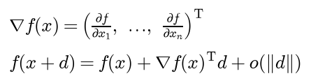
The gradient of f at x is the column of the partial derivatives of f with respect to x1 through xn; and f of x plus d equals f of x plus the gradient transposed times d plus terms that vanish faster than the length of d

The rate of change along a direction d is the directional derivative, and the Cauchy-Schwarz inequality bounds it for every unit direction:

The directional derivative of f at x along d is the limit as t goes to zero of f of x plus t d minus f of x over t, which equals the gradient transposed times d; for a unit vector d this is at most the length of the gradient

Equality holds exactly when d is the gradient divided by its length. The gradient therefore points in the direction of steepest ascent, its length is the slope in that direction, and minus the gradient is the direction of steepest descent. Along a direction tangent to the contour line through x the function does not change to first order, so the gradient is perpendicular to the contour lines, as long as the plot uses the same scale on both axes.

The Jacobian and the Hessian¶

For a map F from n variables to m variables, the Jacobian holds every first partial derivative, one row per output and one column per input. The Hessian of a scalar function is the Jacobian of its gradient:

The Jacobian of F has entry i, j equal to the partial derivative of the i-th output with respect to the j-th input, and F of x plus d equals F of x plus the Jacobian times d plus a small remainder; the Hessian of f has entry i, j equal to the second partial derivative of f with respect to xi and xj

For a scalar function the Jacobian is the single row ∇f(x)'. The Hessian is symmetric when the second partial derivatives are continuous (Schwarz's theorem), and its eigenvalues are the curvatures of f along its eigenvectors: for a unit vector d, the number d'Hd is the second derivative of f along the line through x in direction d, and it always lies between λmin and λmax.

A few gradients and Hessians come up constantly. Here a and b are vectors, A is a square matrix, c a constant, σ the sigmoid applied to each entry, and S the diagonal matrix with entries σ(zi)(1 - σ(zi)):

The third line is the model case for everything below: for symmetric A its gradient vanishes at x = A⁻¹b when A is invertible, and f(x) equals f plus one half of (x - x)'A(x - x). The last line is the logistic regression cost; Logistic regression derives it.

The chain rule¶

If Φ is the composition of a map F from n to m variables followed by a map G from m to q variables, the Jacobians multiply:

A change in xj reaches each output through every intermediate variable ui, and the contributions add. The least-squares gradient in the list above is one application. The residuals r = Xw - y have Jacobian X, and the cost, one over 2N times r'r, has gradient r / N with respect to r, so

The gradient of f with respect to w is the transposed Jacobian of the residuals times r over N, which equals one over N times X transposed times X w minus y, where r is X w minus y and its Jacobian is X

A deep network is a long chain of such maps, and its gradient is a product of many Jacobians. Multiplying them starting from the cost end, one vector-Jacobian product at a time, costs about as much as evaluating the network; this is reverse-mode differentiation, which Backpropagation derives in full.

Taylor approximation and why gradient descent works¶

Taylor's theorem extends the linear approximation by one more term, and for a quadratic the first three terms are exact:

f of x plus d equals f of x plus the gradient transposed times d plus one half d transposed times the Hessian times d plus terms that vanish faster than the squared length of d

Take the step d = -ηg with g = ∇f(x) not zero and η > 0. To first order,

f of x minus eta g equals f of x minus eta times the squared length of g plus terms that vanish faster than eta

and the change, minus η times the squared length of g, is strictly negative. The remainder shrinks faster than η, so for every small enough step size the cost goes down. This is the whole justification of gradient descent; it says nothing yet about how small "small enough" is. The second-order term answers that, with H the Hessian at x:

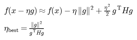
f of x minus eta g is approximately f of x minus eta times the squared length of g plus eta squared over two times g transposed H g; the best step along g is the squared length of g divided by g transposed H g

If g'Hg > 0, this model decreases exactly for steps between 0 and twice the best step, and it is lowest at the best step, the reciprocal of the curvature along g. A step that is too long overshoots the minimum along the line, and twice the best step brings the model back to where it started.

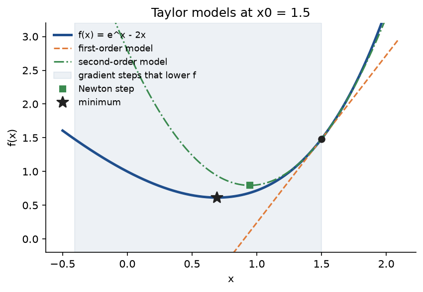
The function e to the x minus 2x near x0 = 1.5 with its tangent line and its second-order Taylor model; the shaded band marks the gradient steps that lower f, the square marks where the Newton step lands at the bottom of the quadratic model, and a star marks the true minimum at ln 2

The figure, from examples/curvature.py, shows both models of f(x) = eˣ - 2x at x0 = 1.5, where f' = 2.4817 and f'' = 4.4817. The tangent line keeps falling forever and says nothing about how far to go; the quadratic model has a bottom, at 0.9463, which is where a Newton step lands, close to the true minimum ln 2 = 0.6931. Because the function curves less than the model to the left, a gradient step lowers f for any step size below 0.7690, while the model predicts below 0.4463.

To turn the second-order picture into a guarantee, suppose the gradient is L-Lipschitz, which for a twice-differentiable f means λmax of the Hessian is at most L everywhere. Writing f(z) - f(x) as the integral of the gradient along the segment from x to z gives the descent lemma, and with z = x - ηg it bounds the progress of one step:

The descent lemma: f of z is at most f of x plus the gradient transposed times z minus x plus L over two times the squared length of z minus x; for a gradient step, f of x minus eta g is at most f of x minus eta times one minus L eta over two, times the squared length of g

Every step with 0 < η < 2 / L lowers the cost by an amount proportional to the squared length of the gradient, and the guaranteed decrease is largest at η = 1 / L, where it is the squared length of g divided by 2L.

Stationary points and the second-order test¶

A point where the gradient vanishes is stationary. There the linear term of the Taylor expansion is zero and the Hessian decides: if it is positive definite (every eigenvalue positive) the point is a strict local minimum, if it is negative definite a strict local maximum, and if it has eigenvalues of both signs a saddle point, a minimum along some directions and a maximum along others. If some eigenvalue is zero and none is negative, the test is inconclusive. The function x² - y² has a saddle at the origin, with Hessian diag(2, -2). Saddle points are common in the cost surfaces of neural networks; gradient descent passes them, while Newton's method, as Pitfalls shows, is attracted to them.

Convex sets and convex functions¶

A set is convex if it contains the segment between any two of its points. Half-spaces, balls and intersections of convex sets are convex; an annulus is not. A function on a convex set is convex if every chord lies on or above its graph:

f of theta x plus one minus theta times z is at most theta f of x plus one minus theta times f of z, for theta between 0 and 1

For differentiable functions two equivalent tests are often easier to check: every tangent plane lies below the graph, and the Hessian is positive semidefinite everywhere.

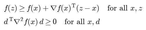
First-order test: f of z is at least f of x plus the gradient transposed times z minus x for all x and z; second-order test: d transposed times the Hessian times d is nonnegative for all x and d

A function is strictly convex if the chord inequality is strict for distinct points and θ strictly between 0 and 1, which a positive definite Hessian guarantees, and μ-strongly convex if the Hessian minus μ times the identity is positive semidefinite everywhere. Convexity survives nonnegative weighted sums, composition with an affine map and pointwise maxima. So the least-squares cost (Hessian X'X / N), the logistic regression cost (Hessian X'SX / N with positive weights in S), the hinge loss of support vector machines and every norm are convex, and adding an L2 penalty, λ / 2 times the squared length of w, makes them λ-strongly convex.

Composition with a nonlinear map does not preserve convexity in general. The squared error of a sigmoid output is not convex in the weight (see Pitfalls), and the cost of a network with a hidden layer is in general not convex in its weights: permuting the hidden units gives distinct minimizers with the same cost, while the average of two such minimizers is usually worse, which convexity would forbid.

Why convexity makes local minima global¶

Let f be convex and x a local minimum, so that f(x) ≤ f(z) for every z within some distance r of x, and suppose some point y had f(y) < f(x). The points zθ on the segment from x to y approach x as θ goes to zero, so for small θ > 0 they lie within distance r, and convexity gives

f of z theta is at most one minus theta times f of x plus theta times f of y, which is less than f of x, where z theta is one minus theta times x plus theta times y

which contradicts local minimality. Hence every local minimum of a convex function is a global minimum. Three consequences are used throughout:

For a differentiable convex f, a vanishing gradient is sufficient for a global minimum: the first-order test with ∇f(x) = 0 reads f(z) ≥ f(x) for every z.
The set of minimizers is convex, and a strictly convex function has at most one minimizer.
Any method that reliably finds a stationary point of a convex function has found the answer, whatever its starting point. Without convexity, gradient descent finds a stationary point that depends on the start, and nothing certifies that it is the best one.

Gradient descent with a fixed step size¶

Gradient descent repeats one update, computing the whole gradient at the current point before moving any coordinate:

The next iterate is the current iterate minus eta times the gradient at the current iterate

One iteration of gradient descent and Newton's method: compute the gradient at the current point; if it is short enough, stop; otherwise take the direction minus g for gradient descent or solve H d = -g for Newton, choose a step length, fixed or halved until f falls enough, and move to the new point

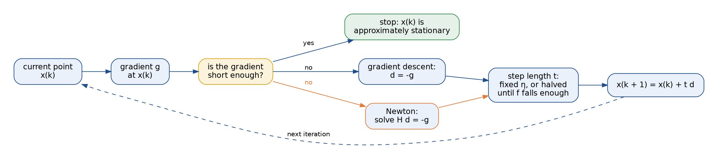
The diagram shows the loop that the package's gradient_descent and newton_method share. The two methods differ only in the direction they move in; the stopping test and the update are the same.

On the quadratic f(x) = ½x'Ax - b'x + c with A symmetric positive definite, the gradient is Ax - b = A(x - x*), so the error obeys a linear recursion. Write A in its spectral decomposition, the sum over i of λi vi vi' with orthonormal eigenvectors vi (see Linear algebra for machine learning), and let ci(k) be the component of the error e(k) along vi. Because vi is an eigenvector of I - ηA with eigenvalue 1 - ηλi, the components evolve independently:

The error after k plus one steps is the error minus eta A times the error, which is I minus eta A times the error, so the error after k steps is I minus eta A to the power k times the initial error; the component along the i-th eigenvector is multiplied by one minus eta lambda i at every step, and the excess cost is one half the sum over i of lambda i times the squared component

Each component shrinks if and only if the size of 1 - ηλi is below one, that is 0 < η < 2 / λi. The binding constraint comes from the largest eigenvalue, and for a quadratic L = λmax:

Gradient descent converges from every start if and only if the step size lies strictly between 0 and 2 over L

Above 2 / L the factor 1 - ηλmax is below -1: the component along the top eigenvector changes sign and grows at every step, the iterates bounce across the valley with increasing amplitude and the cost grows geometrically. At exactly 2 / L the bounce neither grows nor shrinks. Between 1 / L and 2 / L the factor is negative but smaller than one in size, so the iterates oscillate across the valley and still converge; oscillation alone is not divergence.

The speed is set by the slowest component, through the contraction factor ρ:

The contraction factor rho of eta is the largest over i of the size of one minus eta lambda i, which is the larger of the sizes of one minus eta lambda min and one minus eta lambda max; the error after k steps is at most rho to the power k times the initial error

Small steps leave 1 - ηλmin close to one; large steps push 1 - ηλmax towards -1. The two balance at the best fixed step:

The best fixed step is 2 over lambda min plus lambda max, where the contraction factor is kappa minus one over kappa plus one, with kappa equal to L over mu

The common choice η = 1 / L gives ρ = 1 - 1 / κ instead. Reducing the error by a factor of 10 to the power p takes about p ln 10 / (-ln ρ) steps, roughly κ p ln 10 / 2 at the best step and κ p ln 10 at 1 / L when κ is large. The condition number, not the dimension, sets the cost of gradient descent.

Beyond quadratics the same constants govern the standard guarantees, the first for convex f with an L-Lipschitz gradient and η ≤ 1 / L, the second when f is also μ-strongly convex:

For convex f and step at most 1 over L, the excess cost after k steps is at most the squared initial distance to the minimizer divided by 2 eta k; for strongly convex f, the squared distance to the minimizer after k steps is at most one minus eta mu to the power k times the initial squared distance

For non-convex f, the smallest gradient length among the first k iterates falls like one over the square root of k, which guarantees an approximately stationary point and nothing more. Near a minimizer every smooth function looks like its second-order Taylor model, so 2 divided by λmax of the Hessian at the minimizer is the local stability limit. In practice the loop stops when the gradient length falls below a tolerance, preferably relative to its initial length, or after a fixed budget of steps. A cost that has stopped changing is not a reliable signal (see Pitfalls).

Conditioning and feature scaling¶

For least squares the Hessian is X'X / N, so its conditioning is a property of the data. (Linear regression treats the model itself, with the normal equation and ridge regularization.) With an intercept and one feature of mean m and variance s², the matrix X'X / N has rows (1, m) and (m, m² + s²), so

The product of the two eigenvalues is s squared, their sum is one plus m squared plus s squared, and the condition number is approximately one plus m squared plus s squared, squared, divided by s squared

When the feature is far from zero relative to its spread, the two columns of X are nearly parallel: for m = 3 and s = 1 the condition number is about 120. Several features on different scales make it worse, since each feature's variance sets a separate eigenvalue scale: a feature measured in thousands next to one measured in thousandths gives κ of order 10¹². The cost surface becomes a narrow canyon, the step size is capped by the steep direction and progress along the flat direction is negligible.

Standardizing each feature with the mean mj and standard deviation sj of the training data makes the columns zero-mean with unit variance. The intercept decouples from the features, and X'X / N becomes the correlation matrix of the features with a one for the intercept, which for a single feature is the identity: κ = 1, and one step with η = 1 lands on the minimizer. Weights fitted on standardized features map back to raw-feature weights with identical predictions:

The standardized feature is the feature minus its mean, divided by its standard deviation; the raw slope is the standardized slope divided by the standard deviation, and the raw intercept is the standardized intercept minus the sum over features of the standardized slope times the mean divided by the standard deviation

Correlated features still leave κ > 1, since nearly collinear columns give small eigenvalues that no per-feature scaling removes; an L2 penalty bounds λmin from below by λ.

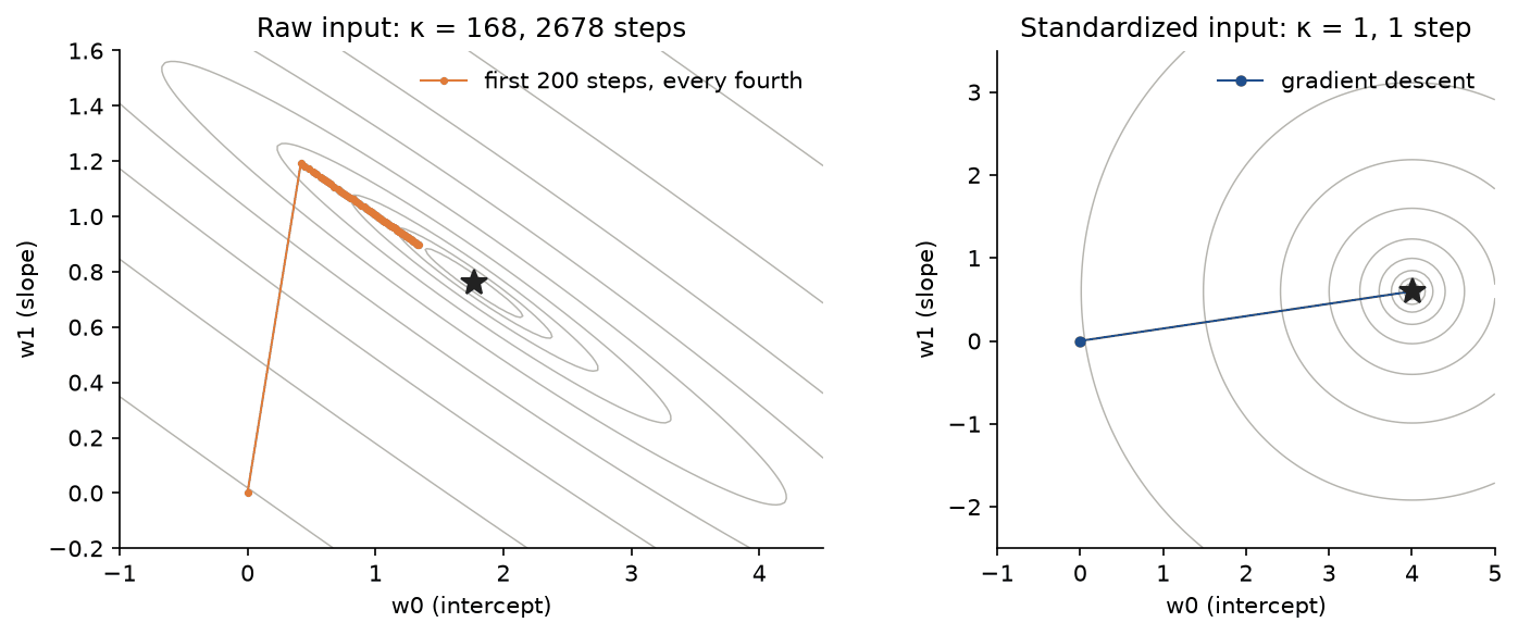
Two panels of contour lines for a line fit with inputs centred near 3. Left, raw input: long thin ellipses, and the gradient descent path jumps once across the valley and then creeps along its floor, 2678 steps in all. Right, standardized input: circular contours, and a single step goes straight to the minimum

The figure, from examples/conditioning.py, fits a line to forty points whose inputs have mean 2.9396 and variance 0.6196. On the raw input κ = 167.9 and gradient descent with η = 1 / L needs 2678 steps to bring the gradient below 10⁻⁸; on the standardized input κ = 1 and one step suffices. Rescaling the variables is the same as running gradient descent with a different step size for each direction, a diagonal preconditioner. Newton's method below uses the inverse Hessian as the preconditioner, which removes the conditioning of a quadratic completely.

Stochastic and mini-batch gradient descent¶

Training costs are averages over examples, f(w) = (1/N) times the sum of the per-example costs fi(w), so the full gradient costs a pass over all N examples. A mini-batch 𝓑 of B indices drawn uniformly at random gives an unbiased estimate, because each example is equally likely to be included, and its error depends on the spread σ² of the per-example gradients:

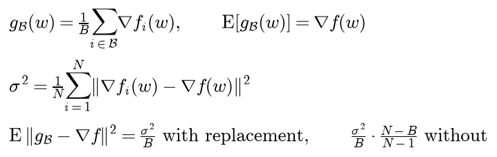
Without replacement the error vanishes for B = N. Stochastic gradient descent uses B = 1, mini-batch gradient descent a moderate B, and an epoch is one pass over the data, usually in a fresh random order. The batch gradient must be the average, not the sum, or the effective step size changes with B.

The noise changes what a constant step size achieves. Near the minimizer the true gradient is small but the estimate is not, so the iterates keep moving: with a constant η they converge to a neighbourhood of x rather than to x. For strongly convex problems and sampling with replacement, the expected excess cost settles at a level proportional to ησ² / B (Bottou, Curtis and Nocedal, 2018). Reaching the minimizer itself needs decreasing steps that satisfy the Robbins-Monro conditions:

The sum of the step sizes is infinite and the sum of their squares is finite, for example eta t equal to eta zero over one plus t over tau

The steps can then travel any distance, but their noise adds up to a finite amount, and the example schedule gives an excess cost of order 1 / t for strongly convex problems. Each stochastic step costs B / N of a full gradient, so on large data sets many cheap noisy steps beat a few exact ones. Optimizers continues from here with momentum, RMSProp, Adam and learning-rate schedules.

Newton's method¶

Newton's method minimizes the second-order Taylor model at each step. Setting the gradient of the model with respect to the step d to zero gives a linear system, solved rather than inverted:

The Hessian at the current iterate times the Newton step equals minus the gradient, and the next iterate is the current one plus the step; in one variable, the next iterate is the current one minus the first derivative divided by the second derivative

In one variable this is Newton's root-finding method applied to f'. For a quadratic the model is exact, so a single step lands on x* = A⁻¹b from any start, whatever the condition number.

Near a minimizer with positive definite Hessian the convergence is quadratic. In one variable, write x for the current iterate and e = x - x for its error, expand f' around x and evaluate at x = x - e, where f'(x) = 0; then ξ is some point between x and x:

Zero equals the first derivative at x minus the second derivative at x times e plus one half the third derivative at xi times e squared; so the new error is e minus f prime over f double prime, which equals f double prime times e minus f prime, over f double prime, which equals the third derivative at xi over twice the second derivative at x, times e squared

The error is squared at every step, and the ratio of the new error to the square of the old one tends to f'''(x) / 2f''(x). Once the error is small, the number of correct digits roughly doubles per step. In n dimensions the same argument bounds the new error by M / 2μ times the squared old error near x*, where M is a Lipschitz constant of the Hessian and μ a lower bound on its smallest eigenvalue.

Newton's method is also affine invariant: rescaling or rotating the variables, x = Tz, changes its iterates by the same transformation, so feature scaling does not affect it. The price is the Hessian: n² numbers to store and a linear solve costing on the order of n³ operations per step, affordable for thousands of parameters and impossible for millions. Two further weaknesses matter. Far from the minimizer the quadratic model can be a poor guide and the full step can increase the cost or diverge, which a backtracking line search repairs by halving the step t until the Armijo condition holds:

f of x plus t d is at most f of x plus c times t times the gradient transposed times d, with c equal to ten to the minus four

And Newton's method only solves ∇f = 0, so it converges just as happily to a saddle point or a maximum when the Hessian is not positive definite. Quasi-Newton methods such as BFGS and L-BFGS build an approximation of the inverse Hessian from successive gradients, trust-region methods restrict the step to where the model is trusted, and Gauss-Newton replaces the Hessian of a least-squares cost by Jr'Jr / N, with Jr the Jacobian of the residuals.

Constrained optimization: Lagrange multipliers¶

Consider minimizing f(x) subject to equality constraints hj(x) = 0 for j from 1 to p. At a constrained minimizer x, moving along the constraint surface must not decrease f to first order. If the gradients of the hj at x are linearly independent, the directions d tangent to the surface are exactly those orthogonal to every one of them. For all of these, ∇f(x*)'d must vanish, or d or -d would lead along the surface to lower values. A vector orthogonal to every direction that is orthogonal to the gradients of the hj lies in their span, so there are multipliers νj with

The gradient of f at the minimizer plus the sum over j of nu j times the gradient of h j at the minimizer is zero; the Lagrangian is f of x plus the sum over j of nu j times h j of x

With one constraint, this says that ∇f is parallel to ∇h: the contour of f through x* touches the constraint surface there. Setting the gradient of the Lagrangian with respect to x to zero gives the condition above, and setting its gradient with respect to ν to zero gives back the constraints.

The multiplier has a meaning. If the constraint is a'x = u and f*(u) is the best value as a function of the level u, then moving u by Δu moves the optimum by some Δx with a'Δx = Δu, and

The change in the optimal value is approximately the gradient of f at the minimizer times delta x, which is minus nu times a transposed delta x, which is minus nu times delta u; so the derivative of the optimal value with respect to the level is minus nu

The multiplier is the price of the constraint: the rate at which the best achievable cost would improve if the constraint were relaxed. For a quadratic objective ½x'Ax - b'x and linear constraints Cx = u, the conditions are linear and form one symmetric system in x and ν:

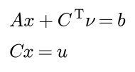
A x plus C transposed nu equals b, and C x equals u

The first line is stationarity of the Lagrangian and the second the constraints themselves. The matrix of the whole system has A in the top left block, C' beside it, C below it and zeros in the bottom right; equality_constrained_quadratic builds it and solves it in one call.

Inequality constraints and the KKT conditions¶

Now minimize f(x) subject to gi(x) ≤ 0 for i from 1 to m and hj(x) = 0 for j from 1 to p, with Lagrangian f + Σ αi gi + Σ νj hj. Under a constraint qualification, a local minimizer x* has multipliers that satisfy the Karush-Kuhn-Tucker conditions:

The four KKT conditions: stationarity, the gradient of f plus the sum of alpha i times the gradients of g i plus the sum of nu j times the gradients of h j is zero; primal feasibility, every g i is at most zero and every h j is zero; dual feasibility, every alpha i is nonnegative; complementary slackness, alpha i times g i is zero for every i

Complementary slackness says that each inequality is either active, gi(x) = 0, and then it may carry a positive multiplier, or inactive, gi(x) < 0, and then αi = 0 and it plays no role, as if it were absent. Dual feasibility fixes the sign: at the optimum minus the gradient of f is a nonnegative combination of the gradients of the active constraints, so the descent direction points out of the feasible region. A candidate with a negative multiplier is not optimal: the constraint is pulling the solution towards the feasible interior, and the solution improves by letting it go.

The usual constraint qualification is linear independence of the gradients of the active constraints. For a convex problem, with f and every gi convex and every hj affine, Slater's condition (some strictly feasible point exists) also suffices, and then the KKT conditions are not only necessary but sufficient: any point that satisfies them is a global minimizer. For small problems this suggests a complete method, which inequality_constrained_quadratic implements:

The active-set method: guess which inequalities are active, hold them as equalities and solve the Lagrange system, check that every inequality is satisfied and that every multiplier of an active inequality is nonnegative; a guess that passes both checks is a KKT point and is kept if its cost is lowest, otherwise it is rejected and the next subset is tried

Trying every subset of m inequalities costs 2ᵐ linear solves, fine for the handful a teaching example has; practical solvers move between subsets one constraint at a time. The multipliers also define the Lagrange dual function q(α, ν), the infimum over x of the Lagrangian, which is a lower bound on f* for every α ≥ 0 and equals it at the optimal multipliers for convex problems satisfying Slater's condition. Support vector machines are the best-known use: the dual variables of the margin constraints are KKT multipliers, complementary slackness makes them zero for every point off the margin, and the points with nonzero multipliers are the support vectors.

Numerical differentiation¶

Finite differences approximate a derivative from function values, and the Taylor expansion shows how accurate they are:

The forward difference, f of x plus delta minus f of x over delta, equals the derivative plus delta over two times the second derivative plus a term of order delta squared; the central difference, f of x plus delta minus f of x minus delta over two delta, equals the derivative plus delta squared over six times the third derivative plus a term of order delta to the fourth

In the central difference the even terms of f(x + δ) and f(x - δ) cancel, so its truncation error falls like δ² instead of δ, and it is exact for quadratics. A partial derivative uses the same formula along one coordinate, so a full gradient costs 2n evaluations of f.

The step cannot be made arbitrarily small. Each function value carries a rounding error of about ε|f|, and dividing a difference of two nearly equal numbers by a small δ amplifies it to about ε|f| / δ. Adding the two error sources gives a V-shaped total for each scheme:

When f and its derivatives are of order one, the best forward step is of order 10⁻⁸ and leaves an error of order 10⁻⁸, while the best central step is of order 10⁻⁵ and leaves an error of order 10⁻¹¹. Finite differences are too expensive and too inaccurate to train with, but they are the standard check of analytic or automatic gradients. Compare the analytic gradient ĝ with the numerical one g through their relative error:

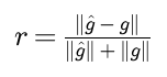
The relative error is the length of g hat minus g divided by the sum of the lengths of g hat and g

With central differences in double precision, values below 10⁻⁷ pass, and values above 10⁻⁴ almost always mean a bug.

Worked example¶

Fit a line, w0 + w1 x, to four points by minimizing the mean squared error:

f of w is one over 2N times the sum over the four points of w0 plus w1 xi minus yi, squared, which is one over 2N times the squared length of X w minus y, with N equal to 4

The inputs are x = (-1, 0, 2, 3) and the targets y = (0, -1, 7, 6), so the design matrix X has the rows (1, -1), (1, 0), (1, 2) and (1, 3), a column of ones for the intercept and a column of inputs. All values below are computed in double precision. Integers and exact binary fractions are shown exactly; other values are rounded to four decimals.

The cost as a quadratic, its gradient and Hessian¶

X'X has the entries N = 4, the sum of the inputs, 4, and the sum of their squares, 1 + 0 + 4 + 9 = 14. X'y is the pair (sum of the targets, sum of input times target) = (12, 32), and y'y = 86. Expanding the square writes the cost as a quadratic, with H having the rows (1, 1) and (1, 3.5):

f of w is one half w transposed H w minus b transposed w plus c, with H equal to one quarter of X transposed X, b equal to one quarter of X transposed y, which is (3, 8), and c equal to y transposed y over 8, which is 86 over 8 or 10.75

Start at w(0) = (0, 0), where every prediction is zero, the residuals Xw(0) - y are (0, 1, -7, -6) and the cost is 10.75. By the chain rule, the gradient g(0) is one quarter of X' times the residuals:

g at step 0 is one quarter of X transposed r, which is one quarter of (0 plus 1 minus 7 minus 6, 0 plus 0 minus 14 minus 18), which is (-3, -8)

This is also Hw(0) - b. Its length is the square root of 73, 8.5440, and the direction of steepest ascent is the gradient divided by its length, (-0.3511, -0.9363): raising both the intercept and the slope lowers the cost, the slope about 2.7 times as fast. The Hessian is the constant matrix H, and central differences of the gradient reproduce it to rounding error.

Taylor models along the negative gradient¶

Along the line w(0) - ηg(0) two numbers are needed, the squared length of g(0), 73, and the product g(0)'Hg(0):

g at step 0 transposed, times H, times g at step 0 is 3 times 3 plus 8 plus 8 times 3 plus 28, which is 281; so the cost along the line is 10.75 minus 73 eta plus 140.5 eta squared

The second-order model is exact here; the first-order model drops the last term.

For η = 0.01 the first-order model gives 10.02 and the exact cost is 10.03405, so the linear model is off by 0.01405.
For η = 0.25 the first-order model gives -7.5, impossible for a sum of squares, while the exact cost is 1.28125.

The curvature along g(0) is 281 / 73 = 3.8493, so the best step along this line is 73 / 281 = 0.2598, and any η between 0 and 0.5196 lowers the cost.

Eigenvalues, the stability limit and the best fixed step¶

H has trace 4.5 and determinant 3.5 - 1 = 2.5, so its eigenvalues are

lambda equals 4.5 plus or minus the square root of 4.5 squared minus 4 times 2.5, all over 2, which is 4.5 plus or minus the square root of 10.25, over 2

that is λmax = 3.8508 and λmin = 0.6492, with unit eigenvectors vmax = (0.3310, 0.9436) and vmin = (0.9436, -0.3310). Both eigenvalues are positive, so H is positive definite, the cost is strictly convex and its one stationary point is the global minimum. Therefore L = 3.8508, μ = 0.6492, κ = 5.9314, the stability limit 2 / L is 0.5194, the best fixed step is 2 / 4.5 = 0.4444, and its contraction factor is (κ - 1) / (κ + 1) = 0.7115.

The curvature along g(0), 3.8493, is close to λmax because g(0) points almost along vmax; that is why the single-step limit 0.5196 is close to, but not the same as, the many-step limit 0.5194. The minimizer solves Hw = b: w = (1, 2), with cost 1.25. The initial error w(0) - w = (-1, -2) splits into -2.2183 times vmax plus -0.2816 times vmin. Five step sizes, with the factors along vmax and vmin and the contraction factor:

η = 0.25: factors 0.0373 and 0.8377, contraction 0.8377. Smooth convergence, limited by vmin.
η = 0.4444: factors -0.7115 and 0.7115, contraction 0.7115. The fastest fixed step.
η = 0.5: factors -0.9254 and 0.6754, contraction 0.9254. Oscillates along vmax and converges slowly.
η = 0.53: factors -1.0409 and 0.6559, contraction 1.0409. Diverges.
η = 0.55: factors -1.1179 and 0.6429, contraction 1.1179. Diverges faster.

Three steps of gradient descent¶

With η = 1/4 and integer data every iterate is an exact binary fraction. The first step is w(1) = w(0) - g(0) / 4 = (0.75, 2). There the residuals 0.75 + 2x - y are (-1.25, 1.75, -2.25, 0.75), the cost is (1.5625 + 3.0625 + 5.0625 + 0.5625) / 8 = 1.28125, and the gradient is one quarter of (sum of the residuals, sum of input times residual) = (-0.25, -0.25). Continuing:

k = 0: w = (0, 0), gradient (-3, -8), cost 10.75, error -2.2183 along vmax and -0.2816 along vmin.
k = 1: w = (0.75, 2), gradient (-0.25, -0.25), cost 1.28125, error -0.0828 and -0.2359.
k = 2: w = (0.8125, 2.0625), gradient (-0.125, 0.03125), cost 1.2626953125, error -0.0031 and -0.1976.
k = 3: w = (0.84375, 2.0546875), gradient (-0.1015625, 0.03515625), cost 1.2588958740234375, error -0.0001 and -0.1655.

The error along vmax is multiplied by 0.0373 per step and is gone after three steps; the error along vmin is multiplied by 0.8377 and dominates from the first step on. Multiplying the rounded numbers, -2.2183 × 0.0373 gives -0.0827; at full precision it is -0.0828. Almost all of the progress is made by the first step, and the remaining steps creep along the valley floor.

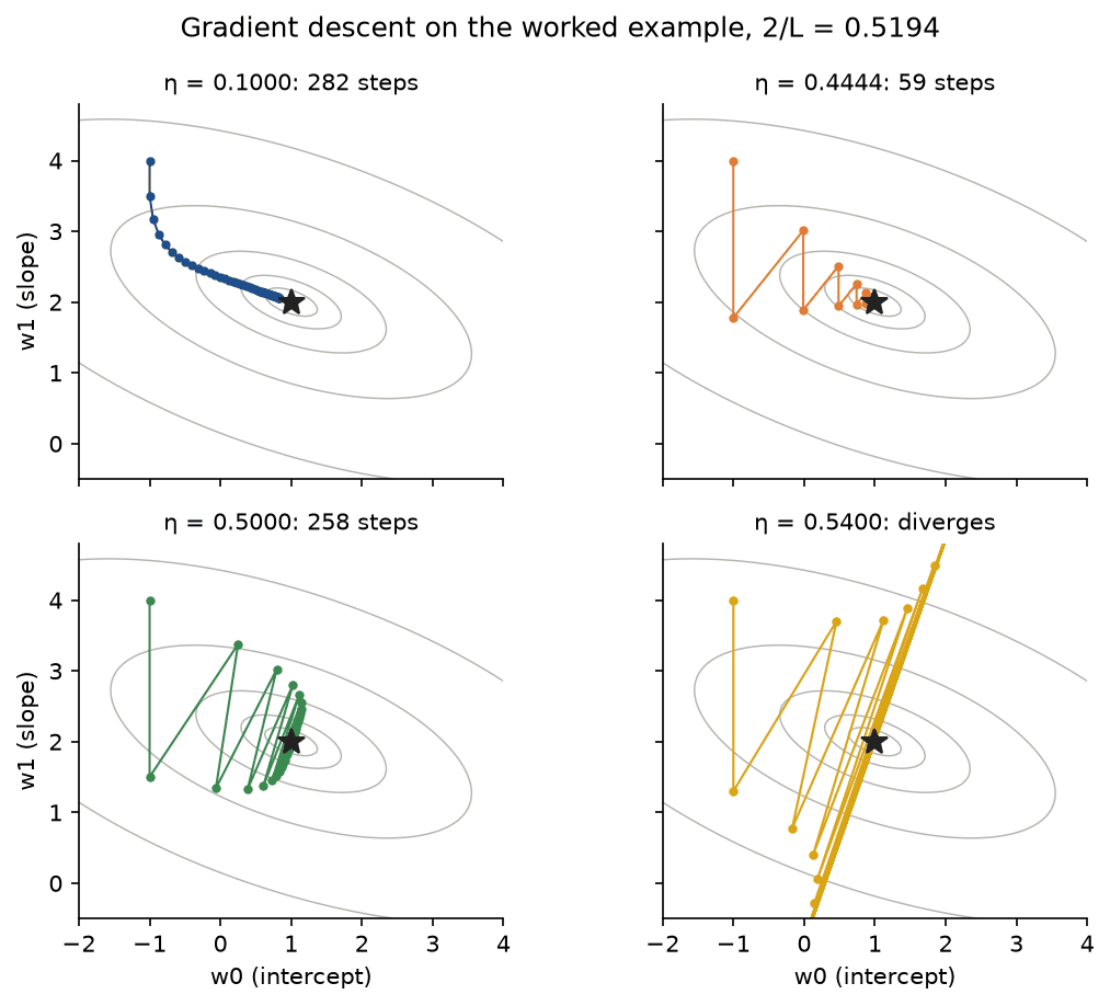
Gradient descent on the worked example from the start (-1, 4) for four step sizes, drawn over the elliptical contour lines: with 0.1 the path bends into the valley and creeps along it in 282 steps, the best fixed step 0.4444 zig-zags to the minimum in 59 steps, 0.5 bounces across the valley for 258 steps, and 0.54 bounces out of the picture

The figure, from examples/step_sizes.py, starts at (-1, 4), where the error has sizeable components along both eigenvectors. The step counts are the steps until the gradient is shorter than 10⁻⁸. With η = 0.54 the factor along vmax is -1.0794, and the iterates leave the picture.

A sweep over step sizes from w(0) confirms the prediction from the contraction factor. The prediction ln(10⁻⁸ / |g(0)|) / ln ρ assumes that the whole initial gradient lies along the slowest direction; each entry gives η, ρ, the predicted and the measured number of steps:

η = 0.05: ρ = 0.9675, predicted 623.2, measured 507.
η = 0.1: ρ = 0.9351, predicted 306.4, measured 250.
η = 0.25: ρ = 0.8377, predicted 116.1, measured 95.
η = 1 / L = 0.2597: ρ = 0.8314, predicted 111.4, measured 91.
η = 0.4444: ρ = 0.7115, predicted 60.4, measured 61.
η = 0.5: ρ = 0.9254, predicted 265.2, measured 266.
η = 0.515: ρ = 0.9832, predicted 1210.4, measured 1211.
η = 0.52 and 0.53: ρ = 1.0024 and 1.0409, both diverge as predicted.

Above the best step the slow direction is vmax, which carries almost all of g(0), and prediction and measurement agree within a step. Below it the slow direction is vmin, which carries only λmin × 0.2816 = 0.1828 of the initial gradient's length; with that value in place of |g(0)| the prediction for η = 0.1 becomes 249.1, against 250 measured. At η = 0.53 the component along vmax runs -2.2183, 2.3090, -2.4035 and so on, growing by exactly 1.0409 per step, and after 200 steps the cost is 8.8 × 10⁷.

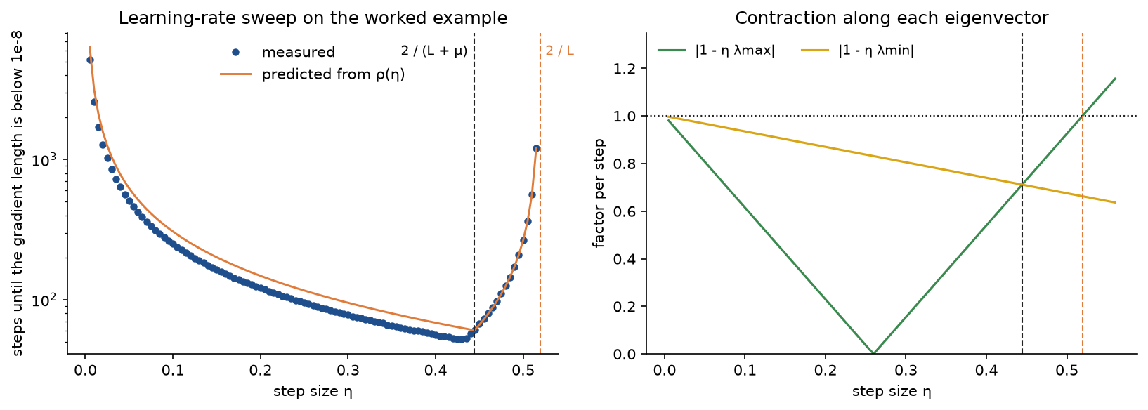
Left: steps to convergence against the step size on a logarithmic axis, measured as dots and predicted as a line, falling to a minimum near the best fixed step and rising sharply towards 2/L. Right: the size of the factor per step along each eigenvector, a V-shaped line for the top eigenvector crossing one at 2/L and a slowly falling line for the bottom eigenvector, meeting at the best fixed step

The right panel explains the left: the number of steps is set by whichever factor is larger, so it falls while the bottom eigenvector dominates and rises once the top one does, and it becomes infinite where the top factor crosses one.

Mini-batch gradients at the start¶

The cost is the average of four per-example costs, one half of (w0 + w1 xi - yi)², and each has its own gradient, the example's row of X times its residual. At w(0) these are (0, 0), (1, 0), (-7, -14) and (-6, -18), whose average is the full gradient (-3, -8). Their spread σ², the mean squared distance from (-3, -8), is (73 + 80 + 52 + 109) / 4 = 78.5. Averaging over all batches of a given size drawn without replacement:

B = 1: the batch gradients average to (-3, -8), with total variance 78.5.
B = 2: average (-3, -8), total variance 78.5 / 2 × 2 / 3 = 26.1667.
B = 3: average (-3, -8), total variance 78.5 / 3 × 1 / 3 = 8.7222.
B = 4: the full gradient itself, with variance 0.

The estimate is unbiased for every batch size, and its variance follows the formula with the finite-population factor (N - B) / (N - 1).

One Newton step¶

The inverse Hessian has the rows (1.4, -0.4) and (-0.4, 0.4), and the Newton step from w(0) is

w at step 0 minus the inverse Hessian times g at step 0 is (1.4 times 3 minus 0.4 times 8, minus 0.4 times 3 plus 0.4 times 8), which is (1, 2), the minimizer

One step from any other start, (5, -7) for instance, lands on the same point, which also solves the normal equations X'Xw = X'y, that is 4w0 + 4w1 = 12 and 4w0 + 14w1 = 32. The best line is 1 + 2x, with residuals (-1, 2, -2, 1).

A constraint and its multiplier¶

Now require the line to pass through (1, 2): h(w) = w0 + w1 - 2 = 0, with gradient a = (1, 1). The unconstrained optimum predicts 3 at x = 1, so the constraint binds. Stationarity of the Lagrangian, Hw - b + νa = 0, together with the constraint is a linear system:

w0 plus w1 plus nu equals 3; w0 plus 3.5 w1 plus nu equals 8; w0 plus w1 equals 2

The first row with w0 + w1 = 2 gives ν = 1. The second row becomes w0 + 3.5w1 = 7, and substituting w0 = 2 - w1 gives 2.5w1 = 5. So w = (0, 2), ν = 1, and the cost is (4 + 1 + 9 + 0) / 8 = 1.75. At this point the gradient Hw - b is (-1, -1) = -νa: it is perpendicular to the constraint line. Because a'H⁻¹a = 1, the best cost on the line w0 + w1 = u is

The optimal cost as a function of the level u is 1.25 plus u minus 3 squared over 2, whose derivative at u equal to 2 is minus 1, which is minus nu

Relaxing the constraint by a small amount Δu lowers the best achievable cost by about Δu, as the multiplier predicts.

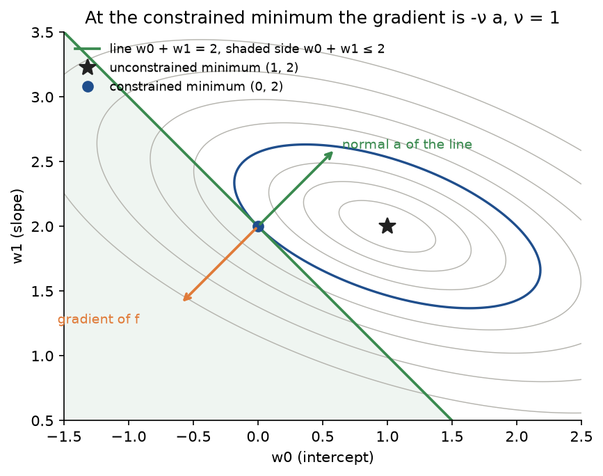
Contour lines of the worked cost with the line w0 + w1 = 2 and the half-plane below it shaded. The highlighted contour through the constrained minimum (0, 2) touches the line there; at that point the gradient arrow points down and to the left and the normal of the line up and to the right, along the same line. The unconstrained minimum (1, 2) is marked with a star

The figure, from examples/constraints.py, shows the tangency: the best contour that still meets the line touches it at (0, 2), and the gradient there is exactly minus ν times the normal. The same constraint written as an inequality, in the form "expression ≤ 0" with a multiplier α ≥ 0:

w0 + w1 - 2 ≤ 0 is active at the solution (0, 2), with α = 1 and cost 1.75. All four KKT conditions hold.
w0 + w1 - 4 ≤ 0 is inactive: the solution is the unconstrained (1, 2), with α = 0 and cost 1.25.
w0 + w1 ≥ 2, written as 2 - w0 - w1 ≤ 0, is also inactive at (1, 2), with α = 0.

For the last constraint, forcing it to be active gives the point (0, 2) again, but with α = -1, which violates dual feasibility: the constraint would be holding the solution back from the interior of the feasible region. Dropping it gives the unconstrained minimum (1, 2), which satisfies 2 - 3 = -1 ≤ 0.

Finite differences by hand¶

With step δ = 0.1 along each coordinate from w(0) = (0, 0):

For the partial derivative with respect to w0, the cost is 10.455 after a step of +δ and 11.055 after -δ. The forward difference is -2.95 and the central difference -3, the exact value.
For the partial derivative with respect to w1, the cost is 9.9675 after +δ and 11.5675 after -δ. The forward difference is -7.825 and the central difference -8, again exact.

The forward differences are off by exactly δ / 2 times the diagonal entry of H, that is 0.05 × 1 and 0.05 × 3.5, the first truncation term; the central differences are exact because the cost is quadratic.

Newton's method on a function that is not quadratic¶

For f(x) = eˣ - 2x the first derivative is eˣ - 2, the second eˣ, and the minimizer is x* = ln 2 = 0.6931. The Newton update is

f of x is exp of x minus 2x, and the next iterate is the current one minus exp of x minus 2, over exp of x, which is the current iterate minus 1 plus 2 exp of minus the current iterate

From x(0) = 0, with the error e(k) = x(k) - ln 2 and the ratio of each error to the square of the previous one:

k = 0: x = 0, error -0.6931.
k = 1: x = 1, error 0.3069, ratio 0.6387.
k = 2: x = 2/e = 0.7358, error 0.0426, ratio 0.4526.
k = 3: x = 0.6940, error 8.95 × 10⁻⁴, ratio 0.4930.
k = 4: x = 0.6931476, error 4.0 × 10⁻⁷, ratio 0.4999.
k = 5: x = 0.6931472, error 8.0 × 10⁻¹⁴.

The ratio of the new error to the square of the old one tends to the third derivative over twice the second derivative at the minimizer, which is exp of x star over twice exp of x star, one half

The ratio approaches 1/2, as the derivation predicts, and the number of correct digits roughly doubles per step: three, six, thirteen. Gradient descent on the same function gains a fixed number of digits per step instead; with η = 0.25 its error runs -0.693, -0.443, -0.264, -0.148, shrinking by a factor that approaches one half per step. Every number in this section is asserted by tests/test_trace.py and printed by examples/worked_example.py.

The code¶

The package calculus_and_optimization is plain NumPy, split into one module per idea. SciPy and scikit-learn are imported only inside the functions of comparisons.py and inside load_breast_cancer_split, so everything else works without them.

arrays.py holds the Array type, the function types and as_vector, which insists that a point is a flat vector.
differentiation.py holds finite_difference with central, forward and backward schemes, numerical_gradient, numerical_jacobian and numerical_hessian built on it, and relative_error and gradient_check.
local_models.py holds directional_derivative, taylor_approximation of first or second order, curvature_along and best_step_along_gradient.
convexity.py holds is_positive_definite by Cholesky factorization, classify_stationary_point from the Hessian's eigenvalues and chord_gap for the convexity inequality.
quadratic.py holds the frozen Quadratic class with its value, gradient, Hessian, minimizer, eigenvalues, smoothness, strong_convexity, condition_number, stability_limit, optimal_step and contraction_factor, and design_matrix and least_squares_quadratic, which build one from data.
descent.py holds gradient_descent, which returns a DescentRun with every point, value, gradient length and step, and predicted_iterations and first_index_below.
newton.py holds newton_method, optionally with backtracking_line_search.
stochastic.py holds minibatch_gradient_descent with reshuffled, with-replacement or fixed-order batches and an optional decaying step, and the per-example gradients and batch spreads of the worked example.
constraints.py holds equality_constrained_quadratic, which solves the Lagrange system, inequality_constrained_quadratic, which enumerates active sets, and kkt_residuals, which measures the four KKT conditions for any candidate.
logistic.py holds the regularized logistic regression cost with its gradient, Hessian and smoothness bound, all leaving the intercept out of the penalty, and logistic_objective, which bundles them.
scaling.py holds fit_standardizer, whose Standardizer maps weights back to raw features.
functions.py holds the small test functions: eˣ - 2x, the saddle x² - y², the square root of 1 + x² and a double well.
datasets.py generates the offset line fits and random quadratic programs and loads the breast cancer split.
worked.py holds the worked example's data, its constraint variants and the helpers that express errors along eigenvectors; trace.py computes every value of the worked example, and report.py formats it.
pitfalls.py holds deliberately wrong code for the Pitfalls section.
comparisons.py calls SciPy's SLSQP, minimize, newton and check_grad and scikit-learn's LogisticRegression.
plotting.py, contour_plots.py and line_plots.py draw every figure in the handbook's four colours and save it reproducibly.

The descent loop in descent.py computes the whole gradient at the current point before moving, and stops on a gradient tolerance, on divergence or when the budget is spent:

while True:
    values.append(evaluate(value, point))
    norms.append(float(np.linalg.norm(current)))
    converged, diverged = finished(point, norms[-1], tolerance)
    if converged or diverged or len(points) > iterations:
        break
    point = point - step_size * current
    current = gradient(point)
    points.append(point)

Newton's method replaces the update by a linear solve, direction = np.linalg.solve(hessian(point), -current), and with line_search=True halves the step until the Armijo condition holds. The examples and the project import the package, so install the repository first as described in the main README. The examples each demonstrate one idea and run in about a second from the repository root:

examples/worked_example.py prints every value of the worked example in the order above, then the normal-equation solution.
examples/step_sizes.py draws the paths and the learning-rate sweep shown above, measures divergence beyond 2 / L and demonstrates the two step-size mistakes of the Pitfalls section.
examples/curvature.py draws the Taylor models and the double-well paths, compares Newton's method with gradient descent, shows Newton's method at a saddle and diverging on a convex function, and checks convexity numerically.
examples/conditioning.py draws the feature-scaling figure and shows a stopping rule fooled by slow progress.
examples/constraints.py draws the constrained minimum, checks the KKT conditions and compares the active-set method with SLSQP on 200 random problems.
examples/finite_differences.py draws the finite-difference errors, checks the chain rule on Jacobians and compares our gradient check with SciPy's on the Rosenbrock function.

python foundations/calculus-and-optimization/examples/worked_example.py
python foundations/calculus-and-optimization/examples/step_sizes.py
python foundations/calculus-and-optimization/examples/curvature.py
python foundations/calculus-and-optimization/examples/conditioning.py
python foundations/calculus-and-optimization/examples/constraints.py
python foundations/calculus-and-optimization/examples/finite_differences.py

The sample project, project/optimizer_race.py, races the methods of this page on one realistic problem: a logistic regression with an L2 penalty on the breast cancer measurements that ship with scikit-learn. It splits the 569 tumours into 400 for training and 169 for testing, checks the gradient and Hessian against finite differences, and then runs Newton's method with a line search and gradient descent with step 1 / L on raw and on standardized features, printing iterations, final cost, wall time and accuracy. It goes on to run full-batch, mini-batch and stochastic gradient descent for 100 epochs, measures the noise floor of constant-step stochastic descent for two sampling schemes, and finally solves the same problem with five SciPy methods and scikit-learn. Options such as --seed, --train-count, --penalty, --max-iterations and --epochs change the setup, and --figures sends the two PNGs to another folder so a custom run does not overwrite the ones shown here; the default run takes about five seconds.

python foundations/calculus-and-optimization/project/optimizer_race.py
python foundations/calculus-and-optimization/project/optimizer_race.py --penalty 0.1 --epochs 50

Its results are discussed under In practice. The notebook calculus_and_optimization.ipynb is a guided tour in the order of this page: the worked example through the package and again in a few lines of bare NumPy, gradient descent on contour plots, Taylor models and Newton's method, convexity, conditioning, mini-batch gradients, constraints, finite differences, each pitfall, and a shortened version of the race. The tests in tests check the worked example value by value, the mathematical properties above and the agreement with SciPy and scikit-learn, and run in a few seconds:

python -m pytest foundations/calculus-and-optimization

The worked example, the line fits and the random problems are defined in code or generated from a seed. The project uses the Breast Cancer Wisconsin (Diagnostic) data set (W. H. Wolberg, W. N. Street and O. L. Mangasarian, 1995, UCI Machine Learning Repository), licensed CC BY 4.0, which ships with scikit-learn as load_breast_cancer, so nothing is downloaded.

In practice¶

Gradient descent and Newton's method on a real problem¶

The breast cancer data have 569 tumours with 30 measurements each, labelled malignant or benign. The measurements live on very different scales: the largest value of a feature ranges from 0.023 to 4254 across the 30 features, and X'X / N with an intercept column has condition number 3.0 × 10¹² on the raw training data and 1.1 × 10⁵ after standardizing. The project fits a logistic regression with an L2 penalty of strength λ = 0.01 on every weight except the intercept:

The cost is the mean over the N examples of the log of one plus e to the zi minus yi zi, plus lambda over two times the sum of the squared weights after the intercept, with z equal to X w; its smoothness constant L is the largest eigenvalue of X transposed X over 4N, plus lambda

The objective is smooth and strongly convex, so every method should reach the same minimizer. The analytic gradient passes a central-difference check with relative errors of 3.7 × 10⁻¹⁰ on raw and 1.3 × 10⁻¹⁰ on standardized features, and the Hessian with 2.0 × 10⁻¹¹. From w = 0 the race gives:

Newton with backtracking, standardized features: 8 iterations to the minimum cost 0.094947, every step of full length.
Gradient descent with η = 1 / L, standardized features (L = 3.244): the gap to the minimum falls below 10⁻⁸ after 1597 iterations, and the gradient below 10⁻⁸ after 3892.
Newton with backtracking, raw features: 10 iterations to 0.098611.
Gradient descent with η = 1 / L, raw features (L = 4.137 × 10⁵): not converged after 20,000 iterations, still 0.107 above the minimum.

The gaps of Newton's method on standardized features are 0.598, 0.153, 0.0601, 0.0173, 0.0026, 9.39 × 10⁻⁵, 1.54 × 10⁻⁷, 4.7 × 10⁻¹³ and then zero to double precision: once the error is small the exponent doubles at each step. Gradient descent on raw features shows conditioning at its worst. The bound L is set by the area features, whose values run into the thousands, so the step size is about 2.4 × 10⁻⁶ and the directions belonging to the small features barely move. Standardizing brings L down to 3.244. The minimized cost differs between the raw and standardized runs because the penalty means something different when the weights refer to differently scaled features: these are two different problems. The standardized model classifies 98.50 % of the training tumours and 97.04 % of the test tumours correctly.

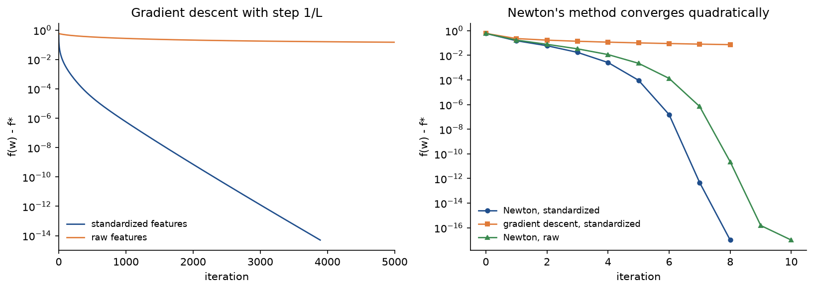
Two details are worth noticing. At the minimizer the Hessian's eigenvalues range only from 0.0096 to 0.2387, so the global bound L = 3.244, which equals the largest curvature at w = 0 where every predicted probability is 0.5, is 13.6 times the largest curvature near the end: η = 1 / L is safe everywhere and conservative near the solution, which is the gap that line searches and adaptive step sizes exploit. And Newton's method needed about the same number of iterations on raw features as on standardized ones, because it is affine invariant; only the penalty, which is not, makes the two problems differ.

Mini-batch gradient descent and its noise floor¶

On the standardized problem the project runs 100 epochs of four settings, measuring the gap f(w) - f* at the end of each epoch. Each entry gives the number of updates, the gap after 10 and after 100 epochs, and the mean gap over epochs 51 to 100:

Full batch with η = 1 / L: 100 updates, 6.17 × 10⁻², 3.55 × 10⁻³, mean 6.30 × 10⁻³.
Batches of 10 with η = 0.1: 4000 updates, 2.01 × 10⁻³, 1.16 × 10⁻⁵, mean 3.12 × 10⁻⁵.
One example per step with η = 0.05: 40,000 updates, 9.68 × 10⁻⁴, 3.78 × 10⁻⁴, mean 1.55 × 10⁻³.
One example per step with ηt = 0.05 / (1 + t / 2000): 40,000 updates, 1.50 × 10⁻⁴, 1.62 × 10⁻⁶, mean 2.58 × 10⁻⁶.

Per pass over the data the stochastic runs are far ahead of full-batch gradient descent, which makes one update per epoch. With a constant step the single-example run stalls at a noise floor around 10⁻³ and jumps around it from epoch to epoch; the decreasing step keeps improving.

How the floor depends on η depends on how the examples are drawn. With one example per step and η = 0.1, 0.05, 0.025 and 0.0125, the mean gap over epochs 51 to 100 is:

Drawn with replacement: 9.41 × 10⁻³, 3.94 × 10⁻³, 1.81 × 10⁻³ and 8.83 × 10⁻⁴, falling by 2.39, 2.17 and 2.06 per halving of η.
Reshuffled every epoch: 6.94 × 10⁻³, 1.55 × 10⁻³, 3.27 × 10⁻⁴ and 5.53 × 10⁻⁵, falling by 4.48, 4.73 and 5.91 per halving.

Sampling with replacement gives the floor proportional to η that the classical analysis predicts. Visiting every example once per epoch in a random order and measuring at the end of each epoch does better, with a floor that falls roughly like η², in line with the analysis of random reshuffling by Mishchenko, Khaled and Richtárik (2020). Reshuffling is what deep-learning data loaders do by default.

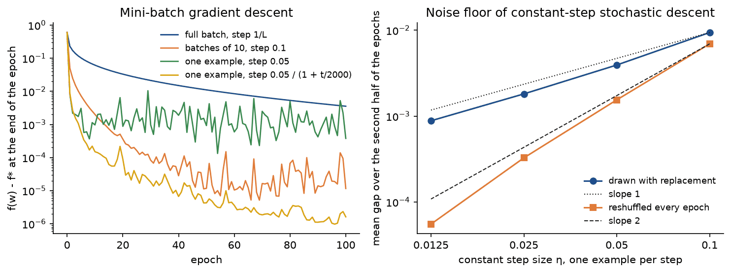
The left panel shows the noise floor directly, and the right panel its slope: the floor of sampling with replacement follows the line of slope one, the floor of reshuffling the line of slope two.

The same problem in SciPy and scikit-learn¶

scipy.optimize.minimize on the standardized problem from the same zero start, with our gradient and, where the method uses one, our Hessian. Each entry gives the iterations, the evaluations of the cost and of the gradient, the gap to our minimum and the largest difference from our Newton weights:

CG: 43 iterations, 160 and 149 evaluations, gap 2.8 × 10⁻¹⁷, weights within 3.1 × 10⁻⁸.
BFGS: 94 iterations, 95 and 95 evaluations, gap 2.5 × 10⁻¹⁶, weights within 7.6 × 10⁻⁸.
L-BFGS-B: 30 iterations, 31 and 31 evaluations, gap 1.4 × 10⁻¹⁵, weights within 1.2 × 10⁻⁷.
Newton-CG: 12 iterations, 12 and 12 evaluations, gap 5.8 × 10⁻¹⁴, weights within 1.4 × 10⁻⁶.
trust-exact: 8 iterations, 9 and 9 evaluations, gap 0, weights within 2.0 × 10⁻¹³.

Every method reaches our minimizer; the differences in the weights reflect each method's stopping tolerance in a flat direction, not a different answer. trust-exact, a trust-region Newton method, takes the same 8 iterations as ours. scikit-learn's LogisticRegression minimizes C times the summed loss plus one half the squared length of the weights, without penalizing the intercept, so C = 1 / (λN) is our problem:

from sklearn.linear_model import LogisticRegression

model = LogisticRegression(C=1.0 / (0.01 * 400), tol=1e-12, max_iter=10_000)
model.fit(standardized_features, labels)

With its default L-BFGS solver it agrees with our weights to 5.2 × 10⁻⁷ and reaches the same 97.04 % test accuracy. The examples add these comparisons, each also covered by a test:

scipy.optimize.newton(lambda x: np.exp(x) - 2, 0.0, fprime=np.exp) returns the same ln 2 as our Newton iteration on eˣ - 2x.
SLSQP (scipy.optimize.minimize(..., method="SLSQP", constraints=...)) gives (0, 2), (1, 2) and (1, 2) for the three inequality versions of the worked example and (0, 2) for the equality version. On 200 random convex quadratic programs in three variables with three random inequality constraints, of which 27, 71, 76 and 26 have zero, one, two and three active constraints at the solution, active-set enumeration and SLSQP agree to within 6.3 × 10⁻⁸.
On the Rosenbrock function scipy.optimize.rosen at (0.3, -1.2), our central-difference check of rosen_der gives a relative error of 4.4 × 10⁻¹¹, and our numerical Hessian matches rosen_hess to 4.2 × 10⁻⁸. scipy.optimize.check_grad reports 3.8 × 10⁻⁷ for the same point: it returns the absolute length of the difference from a forward-difference estimate with step the square root of ε, about 1.5 × 10⁻⁸, which divided by the gradient's length is a relative error of 1.3 × 10⁻⁹.
np.linalg.lstsq and the normal equations give the worked minimizer (1, 2).

When to use which¶

When a closed form exists and the problem is small, use it: np.linalg.lstsq for least squares, not gradient descent.
For smooth problems with up to a few thousand parameters and a cheap Hessian, Newton's method with a line search or a trust region (trust-exact, Newton-CG) converges in a handful of iterations to full precision. Logistic regression fitted this way is iteratively reweighted least squares.
Without a Hessian, L-BFGS is the default workhorse for medium-sized smooth problems; it is scikit-learn's default solver for logistic regression.
Plain full-batch gradient descent is rarely the fastest choice, but it is the building block of everything else and the right mental model for step sizes and conditioning.
For large data sets and neural networks use mini-batch stochastic gradients with momentum or adaptive steps and a schedule, see Optimizers. Exact convergence is not the goal there; generalization is.
For constrained problems use SLSQP or trust-constr for small general problems, specialised quadratic programming solvers (sequential minimal optimization for support vector machines), and projected gradient descent when the feasible set has a cheap projection, such as a box or a ball.
Write gradients analytically or let automatic differentiation compute them, and use central differences only to check them. When f accepts complex arguments, the complex-step derivative, the imaginary part of f(x + iδ) divided by δ, involves no subtraction and stays accurate for steps as small as 10⁻²⁰.

Pitfalls¶

A step size above 2 / L, or a bad estimate of L. On a quadratic, gradient descent converges for every start exactly when η < 2 / λmax; above it the iterates diverge geometrically, and between 1 / L and 2 / L they oscillate but converge. The bound needs the largest eigenvalue, not the largest diagonal entry, which is never larger: on the worked example the largest diagonal entry of H is 3.5, and η = 2 / 3.5 = 0.5714 multiplies the error along vmax by -1.2004 per step, giving a cost of 7.0 × 10¹⁶ after 100 steps, as examples/step_sizes.py prints. When L is unknown, a line search or a short learning-rate sweep, as in the worked example, is safer than a guess.
Updating coordinates one at a time. Updating w0 and then computing the partial derivative for w1 at the new point is not gradient descent but a relaxed Gauss-Seidel sweep, with different iterates and a different stability limit. On the worked example with η = 0.25 the first step goes to (0.75, 1.8125) instead of (0.75, 2), and at η = 0.55 the sequential version converges while gradient descent diverges, so the bug can hide a step size that is too large (examples/step_sizes.py). Compute the whole gradient, then update every parameter.
Judging convergence by the change in the cost. On an ill-conditioned problem the cost falls very slowly long before the minimum. For a line fit with inputs centred at 10 (κ = 16,272) and η = 1 / L, the cost changes by less than 10⁻⁶ per step from step 3168 on, when the weights are (0.4428, 0.9205) against the least-squares (2.0587, 0.7589): the intercept is barely a fifth of its optimal value, and the gradient is still 10⁻⁴ of its initial length. Stop on the gradient length relative to its initial value with a tight tolerance, and check the distance to a reference solution when one is available (examples/conditioning.py).
Skipping feature scaling, or doing it with the wrong statistics. Unscaled features multiply the condition number: from 1 to 168 for a single feature centred near 3, and to 3.0 × 10¹² for X'X / N of the raw breast cancer measurements, against 1.1 × 10⁵ after standardizing, where what remains comes from strongly correlated features such as radius, perimeter and area. Fit the means and standard deviations on the training data only and apply the same transformation to new data (Data leakage and pitfalls), remember that the fitted weights refer to scaled features (Standardizer.weights_to_raw maps them back), and remember that an L2 penalty on raw weights is a different problem from the same penalty on standardized weights.
Assuming a local minimum is global. That holds only for convex functions. On the double well x⁴/4 - x²/2 + y²/2 + 0.15x, gradient descent ends at (-1.0679, 0) with cost -0.4053 or at (0.9143, 0) with cost -0.1061, depending on the start. Convexity is also easy to lose by composition: the squared error of a sigmoid output, (σ(w) - 1)², has second derivative -0.1188 at w = -2 and a chord gap of -0.1686 between w = -4 and w = 0, so it is not convex, while the cross-entropy -ln σ(w) is (Loss functions).

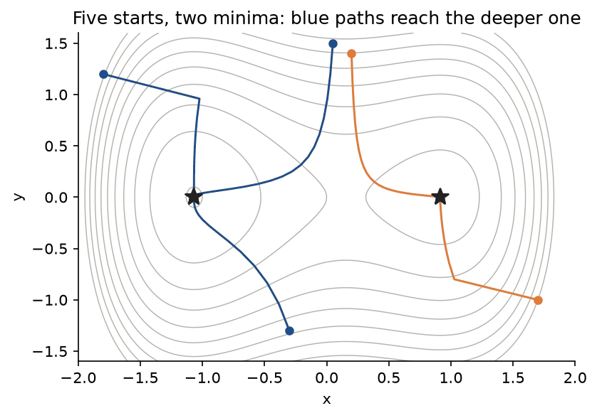
Contour lines of the double well with five gradient descent paths: three blue paths from different starts end at the deeper left minimum, two orange paths end at the shallower right minimum

The figure, from examples/curvature.py, colours each path by the minimum it reaches: which hollow the walk ends in is decided by where it starts.

Trusting pure Newton steps. Newton's method solves ∇f = 0 and does not care what kind of stationary point it finds: on x² - y² one step from (0.7, 0.4) lands on the saddle at the origin, while ten gradient steps move away from it, to (0.0752, 2.4767). Far from the minimum it can diverge even on a convex function: on the square root of 1 + x² the update is x(k + 1) = -x(k)³, which converges from 0.9 (-0.729, 0.3874, -0.0581, ...) and explodes from 1.1 (-1.331, 2.3579, -13.11, 2253, ...). A backtracking line search halves the first step and then converges in four steps (examples/curvature.py). Solve the Newton system with np.linalg.solve or a Cholesky factorization, not by inverting the Hessian, and check that the Hessian is positive definite.
Getting the multipliers wrong. The Lagrange conditions are necessary, not sufficient: minimizing x + y on the unit circle, they hold at (0.7071, 0.7071), the maximum with value 1.4142, as well as at (-0.7071, -0.7071), the minimum with value -1.4142 (examples/constraints.py). For inequalities, the sign condition α ≥ 0 belongs to the convention g(x) ≤ 0 with plus αg in the Lagrangian; flip either and the sign flips. A negative multiplier means that the constraint should be released, as in the worked example's w0 + w1 ≥ 2.
Checking gradients badly. Use central differences with a step near 10⁻⁵ in double precision, and a relative error. For f(x) = eˣ - 2x at x = 1, the central difference has error 4.53 × 10⁻⁵ at δ = 10⁻², 5.66 × 10⁻¹¹ at 10⁻⁵, but 1.03 × 10⁻⁵ at 10⁻¹¹, where rounding dominates; the forward difference bottoms out near 10⁻⁸. Remember that scipy.optimize.check_grad returns an absolute number from forward differences.

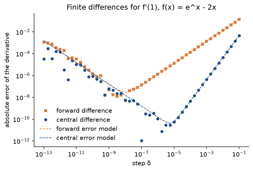
Error of the forward and central differences of e to the x minus 2x at x = 1 against the step on logarithmic axes, with dashed truncation-plus-rounding error models: both are V-shaped, the forward one bottoming out near 10 to the minus 8 at a step near 10 to the minus 8, the central one near 10 to the minus 11 at a step near 10 to the minus 5

The figure, from examples/finite_differences.py, shows the two error models from How it works against the measured errors: the best forward step is near 1.1 × 10⁻⁸ with an error of about 2.9 × 10⁻⁸, the best central step near 5.6 × 10⁻⁶ with about 4.3 × 10⁻¹¹.

Expecting a constant step size to converge stochastically. With a constant step, stochastic and mini-batch gradient descent hover around the minimum at a noise floor that shrinks with η and grows with the gradient variance; it never reaches the minimizer. Decrease the step, increase the batch size, or average the iterates. And average the mini-batch gradient rather than summing it, or the effective step size changes with the batch size (Backpropagation shows how a gradient check catches this).