Localization

A mobile robot with a map has to know where it stands on that map before it can plan a path, and none of its sensors tells it directly. Wheel odometry drifts without bound, and a laser scan only says how far away the nearest surfaces are. Localization fuses the two with Bayes' rule. This page derives the Bayes filter, works a histogram filter on a corridor by hand, builds the odometry motion model and two range-finder sensor models with ray casting written from scratch, and combines them into Monte Carlo localization: a particle filter with low-variance resampling, recovery from kidnapping and a particle count that adapts to the uncertainty. Afterwards you will be able to compute a filter step on paper, implement Monte Carlo localization in NumPy, and read and tune the parameters of the AMCL node in ROS 2 Nav2. It builds on Probability and statistics and Differential-drive kinematics.

To run the code in this topic, install the base group, and the ml group for the two comparisons with SciPy, which are skipped without it.

Intuition

The robot never knows its pose for certain, so it keeps a belief: a probability distribution over every pose (x, y, θ) it could be in, a position in metres and a heading in radians. Two operations update the belief, and they pull in opposite directions.

• Moving blurs the belief. Odometry says "about half a metre forward, turning slightly left", but wheels slip, so every possible pose is shifted by the reported motion and smeared by its uncertainty.
• Sensing sharpens it. Poses from which the map would produce a scan like the one just measured gain probability; poses from which the scan would look different lose it.

The diagram shows the two halves of every update. The odometry enters the prediction and the scan enters the correction; the belief that comes out is the starting point of the next update, so the filter never has to look back further than one step.

A particle filter represents the belief by a few hundred or a few thousand samples, the particles, each a concrete pose hypothesis. Moving pushes every particle through the motion model with its own random noise. Sensing gives every particle a weight: how likely the measured scan is if the robot really stood where the particle stands. Resampling then copies heavy particles and drops light ones, so the samples gather where the probability is.

Three problems of increasing difficulty use the same machinery:

• Position tracking. The start pose is known roughly, and errors stay small as long as the motion noise covers the real slip.
• Global localization. Nothing is known at the start, so the prior is uniform over the free space, and the filter must keep several hypotheses alive until the robot sees something unique.
• The kidnapped robot. The filter believes it knows the pose, but the robot has been carried elsewhere. A confident filter has no particles near the true pose and cannot recover without help.

How it works

Notation

A pose x holds the position and heading. The odometry between two steps is u, given as the pair of poses the odometry reported; a scan z holds K ranges measured along beam angles φ1 to φK relative to the heading; and the map m is an occupancy grid with square cells of side r. The belief after the scan of step t is written bel(x), and the predicted belief, before that scan arrives, carries a bar. The symbol η is a normalizing constant that makes a distribution sum or integrate to one. A particle set has M particles, and particle i has a pose and a normalized weight w. The range the map predicts for a beam is z*, and the sensor's maximum range is z max. The function wrap moves an angle into [-π, π) by adding a multiple of 2π.

The formula images write the step t as a subscript and the particle index i as a superscript in square brackets, so the weight of particle i at step t carries both. In the text these become plain words, such as "the weight w of particle i".

The Bayes filter

The derivation uses only Bayes' rule and the law of total probability. Two assumptions make the problem recursive. The measurement depends only on the current pose, and the pose depends only on the previous pose and the latest control:

Together they say the pose is a complete state, the Markov assumption. Bayes' rule applied to the newest measurement, followed by the first assumption, gives

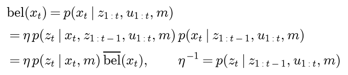
The second factor is the predicted belief. The law of total probability over the previous pose expands it:

The motion assumption removes the earlier scans from the first factor, and the second factor is the belief at the previous step, because the control of step t, issued afterwards, says nothing about where the robot was. The two halves of the filter are

The prediction needs a motion model and the correction a sensor model. The normalizer one over η is the evidence: how probable the filter thought the scan was before it arrived. A low evidence means the scan surprised the filter, which the recovery mechanism below exploits. The Bayes filter applied to a known map is called Markov localization. It leaves open how the belief is stored: as a grid (the histogram filter), as a Gaussian (the Kalman and extended Kalman filters, which cannot represent several hypotheses) or as samples (the particle filter).

The histogram filter

Divide the pose space into cells and the integral becomes a sum. In one dimension, with cells i from 0 to n - 1 and a motion that shifts the robot by s cells with probability p(s), the two equations become

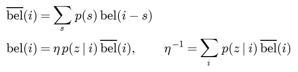
The prediction is a convolution with the motion kernel and the correction an entrywise product followed by normalization. On a corridor that closes on itself the index i - s is taken modulo n; on a corridor with end walls the probability of driving past the end piles up in the last cell. A grid over (x, y, θ) works the same way, but a floor of 24 m by 14 m at 0.1 m and 5 degrees already has 2.4 million cells, almost all of them with negligible probability. A particle filter spends its computation only where the probability is.

The odometry motion model

Odometry integrates wheel rotations into a pose in its own frame, as described in Differential-drive kinematics, and that frame drifts away from the map frame. Only the motion between two readings is trustworthy, so the model expresses it in a form that does not depend on the frame: a rotation towards the direction of travel, a straight translation, and a second rotation to the final heading. For consecutive odometry readings, written with bars and the later one primed,

Each increment is corrupted by zero-mean Gaussian noise whose variance grows with the size of the motion, controlled by four parameters:

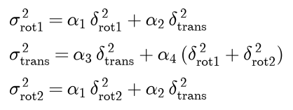
The four parameters describe four physical effects:

• α1, rotation noise caused by rotation: wheel slip while turning, an uncertain wheel base.
• α2, rotation noise caused by translation: unequal wheel radii, drift while driving straight.
• α3, translation noise caused by translation: a wheel radius error, slip on the floor.
• α4, translation noise caused by rotation: sideways scrub while turning.

The standard deviation of each increment is proportional to the motion: with α3 = 0.05 alone, the standard deviation of a translation is √0.05 ≈ 0.22 of its length. Sampling a new pose for a particle at (x, y, θ) draws three standard normal numbers ε1, ε2 and ε3 and subtracts the scaled draws from the increments:

The noisy increments are then applied to the particle:

The increments are applied relative to the particle's own heading θ, not the odometry heading: that is what makes the model usable in the map frame. Two guards matter in practice, and Nav2's differential model has both. When the translation is below 1 cm, the first rotation is set to zero, because the direction of a few millimetres of jitter is meaningless. And the rotations inside the variance formulas are replaced by the smaller of |δ| and |wrap(δ - π)|, so that driving backwards, which decomposes into two half turns, is not treated as two large rotations. The density of the motion model also has a closed form, a product of three Gaussians in the increments, but Monte Carlo localization only ever samples from it.

Ray casting

Both sensor models need the map's view from a pose. Ray casting answers the question for one beam: starting at (x, y) in the direction β = θ + φk, how far is the first occupied cell? Write the ray as the start plus t times the unit vector (cos β, sin β) for t ≥ 0, and let c and ρ be the starting column and row, the cell indices floor(x / r) and floor(y / r). The distance along the ray to the first vertical cell boundary, and the distance between successive vertical boundaries, are

When cos β is zero the ray never meets a vertical boundary and the distance is infinite. The same pair for horizontal boundaries follows with y, ρ and sin β. The traversal repeatedly crosses the nearer boundary: if the next vertical boundary is nearer, it moves one column in the direction of cos β and adds the vertical spacing to that distance, otherwise it moves one row. It stops when it enters an occupied cell, returning the boundary distance at which it entered, or when that distance reaches z max. This is the grid traversal of Amanatides and Woo. It visits exactly the cells the ray passes through, in order, so it never steps over a thin wall the way marching with a fixed step can. A beam costs at most about 2 z max / r steps, and an update casts one beam per particle and per beam of the scan, which is why implementations subsample the scan and why the likelihood field below, which needs no ray casting at all, is the usual default.

The beam model

The beam model treats one range z as the outcome of four competing causes and mixes their densities with weights that sum to one (called z_hit, z_short, z_max and z_rand in the code and in Nav2):

The four causes are:

1. A correct return, measured with noise. The range is Gaussian around z* and cut off to the possible readings. With the normal density written as

the hit component and its truncation factor are

where Φ is the standard normal distribution function. The factor divides by the probability mass the Gaussian keeps inside [0, z max].

1. An object the map does not contain, a person or a chair, blocks the beam early. If such objects are equally likely at every distance, the chance that the beam is still unblocked decays exponentially, so

No reading longer than z* can come from an obstacle in front of the wall.

1. No return at all, from glass, black surfaces or a wall out of range, which the sensor reports as its maximum.
2. Unexplained readings, crosstalk and reflections, described with the other lidar error sources in Sensors for mobile robots.

The last two are a point mass and a uniform floor:

All densities are zero outside the stated ranges. Because the max component is a point mass, the continuous part of the mixture integrates to one minus its weight and the point mass supplies the rest; examples/sensor_models.py checks the total numerically. The random floor matters more than its small weight suggests: it bounds the density of any reading from below by π rand / z max, so a single odd beam cannot drive a particle's weight to zero.

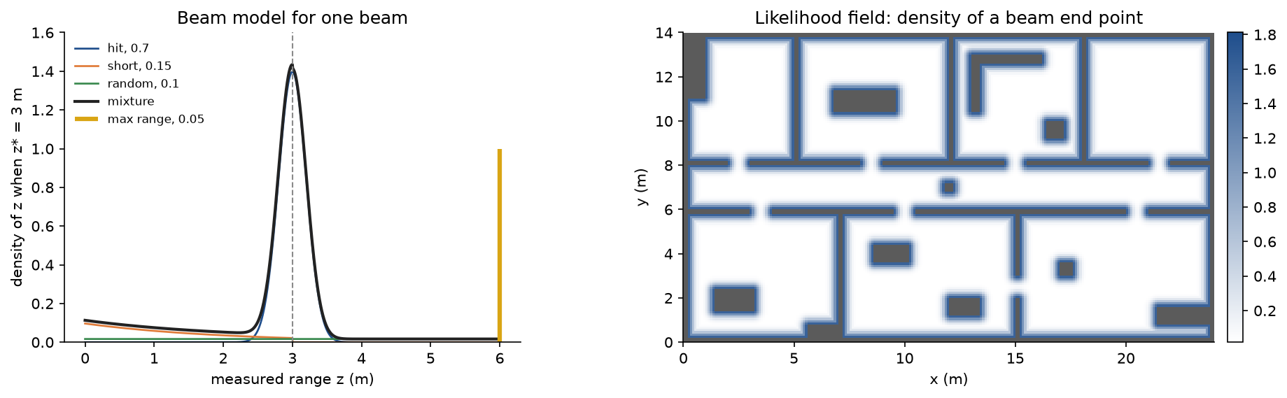
The left panel shows the mixture for an expected range of 3 m: a narrow peak at the wall, an exponential shoulder in front of it for unmapped obstacles, a flat floor everywhere and the point mass at the maximum range. The right panel shows the likelihood field of the next section, which scores a beam's end point by its distance to the nearest wall.

The likelihood-field model

The likelihood field ignores the path of the beam and scores only where it ends. Beam k with range z ends at

Let d be the distance from the end point to the nearest occupied cell, capped at d max. Then

and readings at z max are skipped. The distances form a table computed once per map, the Euclidean distance transform, so an update needs one lookup per beam instead of a ray cast. The model is smooth in the pose, which helps when particles are sparse, but it is not a normalized density over z and it ignores occlusion: an end point behind a wall scores as well as one in front of it. The distance transform is separable. The squared distance of cell (ρ, c) to the nearest occupied cell is a one-dimensional transform along every column followed by one along every row:

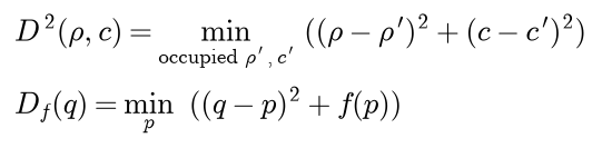
Each one-dimensional transform is the lower envelope of the parabolas rooted at (p, f(p)), which Felzenszwalb and Huttenlocher compute in linear time.

Combining beams

A scan holds many beams, and both models treat them as independent given the pose, so the scan likelihood is a product. A product of a few hundred densities underflows double precision, so the filter works with the log-likelihood ℓ:

and subtracts the largest ℓ over the particles before exponentiating. The independence assumption is false: neighbouring beams hit the same wall, an unmapped person spoils several beams at once, and the map itself is imperfect. The product therefore counts the same evidence many times and is far too confident. The standard remedies are to use only a subset of the beams and to temper the likelihood, raising the product to a power γ ≤ 1:

which treats the K beams as worth K eff independent ones. Every run on this page uses K = 30 beams and γ = 0.05. The beam and likelihood-field models of the AMCL implementation in Nav2, inherited from ROS 1, sidestep the product altogether and score a particle by the heuristic 1 + Σ p³ over its beams.

Monte Carlo localization

A particle set stands for the belief as a weighted sum of point masses, δ here being the Dirac delta:

Importance sampling turns the Bayes filter into operations on samples: draw samples from a proposal distribution that is easy to sample, then weight each by the ratio of the target to the proposal. Take the prediction as the proposal, sampling each particle's previous pose from the previous belief and then its new pose from the motion model, which produces samples from the predicted belief. The target is the corrected belief, so

If the set is not resampled at every step the previous weights carry over, as the second line says, and the weights are normalized to sum to one. One update:

1. Predict. Sample a new pose for every particle from the motion model.
2. Correct. Multiply every weight by the tempered likelihood of the scan. A particle inside an occupied cell gets weight zero.
3. Estimate the pose and its covariance from the weighted set.
4. Resample if the weights have become too uneven, or if random particles are to be injected.

The diagram is the loop MonteCarloLocalizer.step runs. Resampling does not add information. It moves the representation of the belief from weights to sample density, so that the next prediction spends particles where the probability is.

Low-variance resampling

Lay the normalized weights end to end on [0, 1), with cumulative sums c. Low-variance resampling draws a single number r uniformly from [0, 1/M) and places M equally spaced pointers:

The interval of particle i has the length of its weight and the pointers are 1/M apart, so the interval contains either the floor or the ceiling of M times the weight: every particle gets its expected number of copies, rounded one way or the other. Since r is uniform, the expected number is exactly M times the weight, so the scheme is unbiased. With equal weights it returns every particle exactly once. The whole sweep costs time proportional to M.

Multinomial resampling, which draws M independent indices with probabilities given by the weights, is also unbiased, but the number of copies of each particle is random:

Even with equal weights one round therefore discards about 37 % of the distinct particles for no reason.

The effective sample size

It equals M when all weights are equal and 1 when one particle holds all of the weight. Estimates from M weighted particles are roughly as accurate as estimates from that many unweighted samples from the target. Selective resampling resamples only when the effective sample size drops below a threshold, commonly M/2. Every resampling step replaces exact weights by random copy counts and removes particles that might have become useful later, so skipping it while the weights are still spread out loses less information. Nav2 instead resamples every resample_interval updates.

The estimate and its covariance

The weighted mean of the positions is the obvious estimate. Headings need a circular mean, and the covariance must measure angular deviations the short way round:

A mean is only meaningful for a cloud with one mode: the mean of two hypotheses in neighbouring rooms lies in the wall between them. Like AMCL, the implementation first groups the particles into clusters. It drops them into bins of 0.5 m by 0.5 m by 10 degrees, joins occupied bins that touch (26 neighbours, wrapping around in heading), and reports the mean and covariance of the cluster with the largest total weight. The estimate is taken from the weighted set before resampling, because resampling only adds noise and injected random particles are not part of the belief. Nav2 publishes this estimate on amcl_pose as a PoseWithCovarianceStamped whose 6 by 6 covariance holds the x, y and yaw entries of the covariance above.

Recovering from failures: augmented MCL

A particle filter that has converged on the wrong place, or whose robot has been carried away, has no particles near the true pose, and no amount of reweighting will create one. Augmented MCL detects the failure from the evidence. The average weight before normalization estimates the evidence, and the filter keeps a slow and a fast exponential average of it:

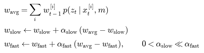
Both averages start at the first average likelihood. During resampling each drawn particle is replaced, with probability

by a pose drawn uniformly from the free space. While scans fit as well as they usually do, the two averages agree and nothing is injected. A sudden drop in fit pulls the fast average below the slow one within a few updates and random particles start to appear; once some of them land near the true pose and win the resampling, the average likelihood recovers, the fast average follows and the injection stops. A fit that stays poor for good, for example after furniture has moved, eventually drags the slow average down as well, which also stops the injection. This implementation computes the average likelihood from the geometric mean of the per-beam likelihoods, the exponential of ℓ / K, instead of from the raw product. That is a monotone change of scale that keeps the average from swinging by orders of magnitude when the number of valid beams changes; any score that drops sharply when the map stops explaining the scans would serve.

KLD-sampling: an adaptive particle count

Global localization needs tens of thousands of particles to have one near every possible pose, while tracking a converged cloud needs a few hundred. KLD-sampling chooses the count at every resampling step. Discretize the pose space into bins. If the true belief occupies k bins and n samples are drawn from it, the likelihood-ratio statistic, 2n times the Kullback-Leibler divergence between the empirical bin frequencies and the true ones, is asymptotically chi-square distributed with k - 1 degrees of freedom. Requiring the divergence, introduced in Information theory, to stay below ε with probability 1 - δ gives

and the Wilson-Hilferty approximation to the chi-square quantile makes it explicit:

with z of 1 - δ the upper δ quantile of the standard normal distribution. For large k the count grows almost linearly, about (k - 1) / 2ε. The true k is unknown, so the algorithm counts occupied bins as it goes: it draws particles one at a time, updates k after each draw, and stops once n exceeds both the bound for the current k and a minimum count, or reaches a maximum. A spread-out cloud keeps opening new bins and grows to the maximum; a converged cloud stops opening bins and the count falls to the bound or the minimum. The bins here are AMCL's, 0.5 m by 0.5 m by 10 degrees. AMCL counts the bins of the resampled particles, as this implementation does, rather than of the particles after the motion update as in the original description; both measure the spread of the belief.

Worked example

A corridor with doors

A corridor of ten cells closes on itself, so moving right from cell 9 enters cell 0. Doors stand at cells 1, 4, 5 and 8. The door detector reports a door with probability 0.65 in front of a door and 0.15 in front of a wall, so it reports a wall with probabilities 0.35 and 0.85. A command to move one cell to the right moves the robot by 0, 1 or 2 cells with probabilities 0.15, 0.75 and 0.10. The robot starts in cell 4 without knowing it, reads "door", moves, reads "door", moves and reads "wall". The prior is uniform, 0.1 per cell.

First correction, "door". Every door cell gets 0.65 × 0.1 = 0.065 and every wall cell 0.15 × 0.1 = 0.015. The evidence is 4 × 0.065 + 6 × 0.015 = 0.35, so door cells now hold 0.065 / 0.35 = 0.1857 and wall cells 0.015 / 0.35 = 0.0429.

First prediction. The predicted belief of a cell is 0.15 times its own belief plus 0.75 times that of the cell to its left plus 0.10 times that of the cell two to the left. For cell 5, fed by cells 5, 4 and 3, that is 0.15 × 0.1857 + 0.75 × 0.1857 + 0.10 × 0.0429 = 0.1714. For cell 6 it is 0.15 × 0.0429 + 0.75 × 0.1857 + 0.10 × 0.1857 = 0.1643, and for cell 2 it is 0.15 × 0.0429 + 0.75 × 0.1857 + 0.10 × 0.0429 = 0.1500.

Second correction, "door". The unnormalized values include 0.65 × 0.1714 = 0.1114 for cell 5, 0.65 × 0.0643 = 0.0418 for cell 1 and 0.15 × 0.1643 = 0.0246 for cell 6, and the ten of them sum to the evidence 0.3321. Cell 5 now holds 0.1114 / 0.3321, which is 0.3354 from the rounded terms and 0.3355 at full precision. Two doors in a row point to cells 4 and 5, and the motion model says the robot most likely went from one to the other.

Second prediction and third correction, "wall". Cell 6 is predicted at 0.15 × 0.0742 + 0.75 × 0.3355 + 0.10 × 0.1258 = 0.2753, multiplied by 0.85 to 0.2340 and divided by the evidence 0.7085 (0.7086 if summed from the rounded beliefs), giving 0.3303. The whole computation, every value rounded to four decimals and listed for cells 0 to 9:

• Prior: 0.1000 in every cell.
• Correct, door: 0.0429, 0.1857, 0.0429, 0.0429, 0.1857, 0.1857, 0.0429, 0.0429, 0.1857, 0.0429; evidence 0.3500.
• Predict: 0.0571, 0.0643, 0.1500, 0.0571, 0.0643, 0.1714, 0.1643, 0.0571, 0.0643, 0.1500.
• Correct, door: 0.0258, 0.1258, 0.0677, 0.0258, 0.1258, 0.3355, 0.0742, 0.0258, 0.1258, 0.0677; evidence 0.3321.
• Predict: 0.0673, 0.0450, 0.1071, 0.0673, 0.0450, 0.1473, 0.2753, 0.0931, 0.0456, 0.1071.
• Correct, wall: 0.0807, 0.0222, 0.1285, 0.0807, 0.0222, 0.0727, 0.3303, 0.1116, 0.0225, 0.1285; evidence 0.7085.

After three readings the most probable cell is 6, where the robot is. Cells 2 and 9 keep 0.1285 each: starting at cell 1 or 8, staying put on the first move and advancing on the second also produces door, door, wall. The evidence records how surprised the filter was by each reading: a second door was less expected than the first, and a wall after two doors was expected.

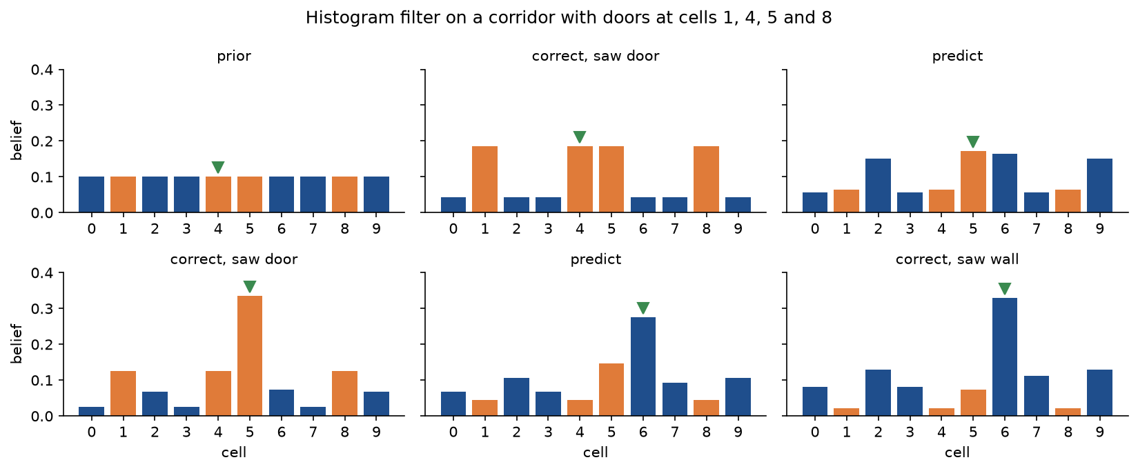
Every correction sharpens the belief and every prediction blurs it. The green marker shows that the peak follows the robot from the second door reading on.

Sampling the motion model

Odometry reports (4.00, 2.00, 0.50) and then (4.36, 2.27, 0.70). The displacement is (0.36, 0.27), so the translation is √(0.36² + 0.27²) = 0.45, the angle of the displacement is atan2(0.27, 0.36) = 0.6435, the first rotation is 0.6435 - 0.50 = 0.1435 and the second rotation is 0.70 - 0.50 - 0.1435 = 0.0565. With α = (0.1, 0.05, 0.05, 0.02) the variances, written to six decimals because their square roots are sensitive to rounding, are:

• First rotation: 0.1 × 0.1435² + 0.05 × 0.45² = 0.002059 + 0.010125 = 0.012184.
• Translation: 0.05 × 0.45² + 0.02 × (0.1435² + 0.0565²) = 0.010125 + 0.000476 = 0.010601.
• Second rotation: 0.1 × 0.0565² + 0.05 × 0.45² = 0.010444.

The standard deviations are therefore 0.1104, 0.1030 and 0.1022. The translation term dominates all three: half a metre of driving makes the heading more uncertain than the small turn does. With the standard normal draws 0.8, -0.5 and 1.2, the noisy increments are 0.1435 - 0.8 × 0.1104 = 0.0552 for the first rotation, 0.45 + 0.5 × 0.1030 = 0.5015 for the translation and 0.0565 - 1.2 × 0.1022 = -0.0661 for the second rotation.

A particle at (2.5, 2.0) facing north, θ = π/2 = 1.5708, turns to 1.5708 + 0.0552 = 1.6260 and drives 0.5015 m. Its new position is x = 2.5 + 0.5015 × (-0.0552) = 2.4723 and y = 2.0 + 0.5015 × 0.9985 = 2.5007, and its new heading is 1.6260 - 0.0661 = 1.5599. In the odometry frame the robot drove north-east, yet the particle moves almost due north: it applies the motion relative to its own heading, which is the whole point of the decomposition.

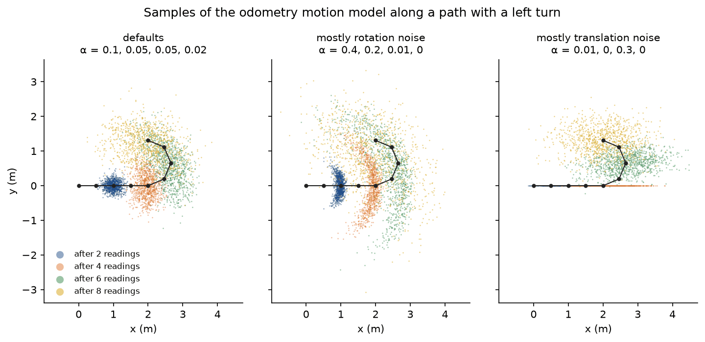
Rotation noise bends the cloud into the familiar banana shape, translation noise stretches it along the path, and the noise of every reading adds up. With the defaults the final cloud has a spread of 0.772 m after eight readings of 0.5 m.

One correction with five particles

Five particles stand in an empty room whose walls lie at x = 0, x = 5, y = 0 and y = 4, all facing east. The scan has two beams, straight ahead and to the left, and reads 2.3 m and 2.2 m. The beam model uses π hit = 0.7, π short = 0.15, π max = 0.05, π rand = 0.1, σ hit = 0.2 m, λ short = 0.5 per metre and z max = 6 m. The expected ranges are 5 - x for the forward beam and 4 - y for the left beam, and the truncation factor of the hit component is 1.0000 to four decimals for all of them.

Particle 3's left beam shows all four components. It reads 2.2 m where the map predicts 3.0 m, four standard deviations short:

• Hit: the normal density 0.8 m from its mean, exp(-0.8² / (2 × 0.04)) / (0.2 √(2π)), which is 1.9947 exp(-8) = 0.000669, shown as 0.0007.
• Short: 0.5 exp(-0.5 × 2.2) / (1 - exp(-0.5 × 3.0)) = 0.1664 / 0.7769 = 0.2142.
• Max: 0, since the reading is not the maximum range.
• Random: 1 / 6 = 0.1667.
• Mixture: 0.7 × 0.0007 + 0.15 × 0.2142 + 0.05 × 0 + 0.1 × 0.1667 = 0.0493.

The short and random components carry this beam: it is just what a person standing in front of the wall would produce. Particle 5's forward beam is a good fit, reading 2.3 m where the map predicts 2.4 m. Its hit density is 1.9947 exp(-0.125) = 1.7603, its short density is 0.5 exp(-1.15) / (1 - exp(-1.2)) = 0.2266 (0.2265 from the rounded quotient 0.1583 / 0.6988), and its mixture is 0.7 × 1.7603 + 0.15 × 0.2266 + 0.1 × 0.1667 = 1.2829. Doing this for all ten beams gives, per particle, the pose, the two expected ranges, the two densities, their product and the normalized weight:

• Particle 1 at (2.2, 1.6): expected 2.8 and 2.4, densities 0.1095 and 0.8993, likelihood 0.0985, weight 0.0388.
• Particle 2 at (2.5, 2.0): expected 2.5 and 2.0, densities 0.8968 and 0.8636, likelihood 0.7745, weight 0.3049.
• Particle 3 at (2.8, 1.0): expected 2.2 and 3.0, densities 1.2489 and 0.0493, likelihood 0.0615, weight 0.0242.
• Particle 4 at (3.1, 2.6): expected 1.9 and 1.4, densities 0.2056 and 0.0171, likelihood 0.0035, weight 0.0014.
• Particle 5 at (2.6, 1.9): expected 2.4 and 2.1, densities 1.2829 and 1.2489, likelihood 1.6022, weight 0.6307.

The likelihoods sum to 2.5402, and each weight is a likelihood divided by that sum. Particle 3's likelihood is 1.2489 × 0.0493 = 0.0616 from the rounded densities and 0.0615 at full precision. Particle 4 shows the job of the random floor. Its left beam reads 2.2 m where the wall should stop it at 1.4 m, four standard deviations too long and beyond anything an obstacle could explain; its density 0.0171 is almost entirely π rand / z max = 0.0167.

The squared weights sum to 0.4929, so the effective sample size is 2.0290 at full precision, and 1 / 0.4929 = 2.0288 from the rounded sum: five particles, but the information of about two.

Low-variance resampling with the offset r = 0.10 places pointers at 0.10, 0.30, 0.50, 0.70 and 0.90 on the cumulative weights 0.0388, 0.3437, 0.3679, 0.3693 and 1.0000. The first two pointers fall in particle 2's interval, from 0.0388 to 0.3437, and the other three in particle 5's interval, from 0.3693 to 1, so the new set holds particle 2 twice and particle 5 three times. That matches the expected copy counts, five times the weights: 0.19, 1.52, 0.12, 0.01 and 3.15, rounded one way or the other.

The estimate from the weighted set is x = 0.0388 × 2.2 + 0.3049 × 2.5 + 0.0242 × 2.8 + 0.0014 × 3.1 + 0.6307 × 2.6 = 2.5595 and y = 1.8980, with heading 0. The covariance has the rows (0.0089, -0.0024, 0), (-0.0024, 0.0268, 0) and (0, 0, 0), standard deviations of 0.0945 m in x and 0.1638 m in y. The off-diagonal entry is -0.00235 to five decimals and comes out as -0.0023 from the rounded weights. The heading row and column are zero because all five particles face east. Most of the spread in y comes from particle 3, which sits 0.898 m below the mean: with a weight of only 0.0242 it still contributes 0.0242 × 0.898² = 0.0195 of the 0.0268.

With the likelihood-field model (π hit = 0.9, π rand = 0.1, σ hit = 0.2 m), particle 2's beams end at (4.8, 2.0) and (2.5, 4.2). Both end points are 0.2 m from the nearest wall surface, the first in front of the wall at x = 5 and the second behind the wall at y = 4, so both get the density 0.9 × 1.2099 + 0.1 / 6 = 1.1055 (1.1056 from the rounded terms). The likelihood field cannot tell an end point behind a wall from one in front of it.

Recovery averages and the KLD bound

With α slow = 0.02, α fast = 0.2, both averages at 0.60 and the average likelihood suddenly dropping to 0.06, the first update gives a slow average of 0.60 + 0.02 × (0.06 - 0.60) = 0.5892, a fast average of 0.60 + 0.2 × (0.06 - 0.60) = 0.4920 and an injection probability of 1 - 0.4920 / 0.5892 = 0.1650. Three updates in a row give:

• Update 1: slow 0.5892, fast 0.4920, injection probability 0.1650.
• Update 2: slow 0.5786, fast 0.4056, injection probability 0.2990.
• Update 3: slow 0.5682, fast 0.3365, injection probability 0.4079.

The last injection probability is 0.4078 from the rounded averages. After three bad scans, four in ten resampled particles are replaced by random poses.

For KLD-sampling with ε = 0.05 and δ = 0.01, the upper quantile is 2.3263. For samples occupying k = 12 bins, a = 2 / (9 × 11) = 0.0202 and its square root is 0.1421, so the bracket is 1 - 0.0202 + 0.1421 × 2.3263 = 1.3105 at full precision (1.3104 from the rounded terms). Its cube is 2.2504 at full precision (2.2502 from the rounded bracket), and n = 11 / (2 × 0.05) × 2.2504 = 247.5, rounded up to 248 particles. For 2, 12, 50 and 200 occupied bins the bound asks for 66, 248, 750 and 2484 particles; with the quantile 0.99 instead, which means δ = 0.161, it asks for 20, 155, 588 and 2188.

Every number in this section is asserted by tests/test_worked_example.py, tests/test_particle_step.py and tests/test_sensor_models.py, and printed by examples/corridor_filter.py, examples/motion_model.py and examples/particle_step.py.

The code

The package localization uses only NumPy and the standard library; SciPy is imported only inside comparisons.py. It is split into one module per idea:

• arrays.py, angles.py and normal.py hold the array types, wrap_angle with the circular mean, and the normal density, distribution function and quantile.
• histogram.py holds the histogram filter: histogram_predict (a convolution with or without wrap-around), door_likelihood, histogram_correct, run_corridor, which keeps every belief, and format_histogram_trace.
• grid.py holds OccupancyGrid, whose rows are y and columns x, so a point falls in the cell (floor(y / r), floor(x / r)), with rectangles_to_grid and wall_with_doors. maps.py builds the 24 m by 14 m floor of the simulated runs and the worked example's room.
• ray_casting.py holds cast_ray, the traversal for one ray as a plain loop, cast_rays, the same traversal for many rays at once on NumPy arrays, and march_ray for checks and for the thin-wall pitfall.
• distance_field.py holds the linear-time distance transform and a brute-force check.
• sensor_models.py holds BeamModel, with components and density, and LikelihoodFieldModel; sensors.py combines a model with a map into BeamSensor and LikelihoodFieldSensor, which return one log-likelihood per particle.
• motion.py holds OdometryNoise, odometry_increments, increment_standard_deviations, apply_increments and sample_odometry_motion, which accepts fixed standard normal draws for hand checks.
• resampling.py holds normalize_log_weights, effective_sample_size, low_variance_resample, its textbook loop and multinomial_resample.
• bins.py, estimation.py, kld_sampling.py and recovery.py hold AMCL's pose bins, the weighted and clustered estimates, the KLD bound and sample count, and the slow and fast averages.
• localizer.py is the heart of the topic: FilterState, uniform_state, gaussian_state and MonteCarloLocalizer with predict, resample and step.
• trajectories.py, simulation.py and runs.py simulate a robot: a unicycle steering towards waypoints, filter updates every 0.25 m or 0.2 rad, odometry with scale errors and drift, scans with noise and bad readings, and run_localizer, which keeps the errors and particle counts of every update.
• worked_example.py and particle_step.py build the worked examples above; pitfalls.py holds the demonstrations of the Pitfalls section.
• nav2.py writes a localizer's settings as a Nav2 AMCL parameter file, and comparisons.py checks two building blocks against SciPy and NumPy's chi-square sampler.
• plotting.py and map_plots.py draw every figure in the handbook's four colours.

The core of one update in MonteCarloLocalizer.step follows the four steps of the algorithm:

particles = state.particles
if previous is not None:
    particles = self.predict(state.particles, previous, current, rng)
log_likelihood = self.sensor.log_likelihood(particles, ranges, angles)
log_weights = np.log(state.weights) + self.likelihood_exponent * log_likelihood
weights = normalize_log_weights(log_weights)
per_beam = np.exp(log_likelihood / max(self.sensor.beams_used(ranges), 1))
average = float(state.weights @ per_beam)

followed by the recovery averages, the clustered estimate and the resampling decision. Low-variance resampling is the pointer comb from How it works, with searchsorted finding for every pointer the first cumulative weight that reaches it:

start = rng.uniform(0.0, 1.0 / count) if offset is None else offset
pointers = start + np.arange(count) / count
cumulative = np.cumsum(weights / weights.sum())
cumulative[-1] = 1.0
return np.searchsorted(cumulative, pointers, side="left").astype(np.int64)

With adaptive=True, resample draws particles in growing blocks, applies the injection to each block, and stops at the first count that kld_enough accepts. Drawing in blocks gives the same distribution as drawing one particle at a time but avoids a Python loop.

The examples and the project import the package, so install the repository first as described in the main README. The examples each demonstrate one idea and run in a second or two from the repository root, except common_mistakes.py, which runs twelve short global localizations and takes about ten seconds:

• examples/corridor_filter.py prints every belief of the corridor example with its evidence and saves the bar charts above.
• examples/motion_model.py prints the motion-model example, checks the sampled spread against the predicted standard deviations and saves the motion clouds.
• examples/sensor_models.py checks ray casting against single rays and fine marching, prints the beam model's components and the total probability of the mixture, checks the distance transform against brute force and saves the sensor-model figure.
• examples/particle_step.py prints the five-particle correction, resampling and estimate, the likelihood-field densities, the recovery averages and the KLD bounds.
• examples/common_mistakes.py demonstrates every pitfall below next to the correct result.
• examples/library_equivalents.py compares the distance transform and the KLD bound with SciPy, the Wilson-Hilferty approximation with NumPy's chi-square sampler, and prints two localizers as Nav2 parameter files.

python robotics/localization/examples/corridor_filter.py
python robotics/localization/examples/motion_model.py
python robotics/localization/examples/sensor_models.py
python robotics/localization/examples/particle_step.py
python robotics/localization/examples/common_mistakes.py
python robotics/localization/examples/library_equivalents.py

The sample project

project/localization_simulator.py applies everything to a robot on a simulated floor, with figure drawing in project/simulator_figures.py. The floor is 24 m by 14 m at 0.1 m per cell, with a corridor, seven rooms, furniture and a pillar. A tour starts at the west end of the corridor and covers 59.1 m in 276 filter updates, one whenever the robot has moved 0.25 m or turned 0.2 rad. Odometry over-reports distance by 3 %, under-reports rotation by 2 %, drifts by 0.015 rad per metre and adds random noise; integrated on its own it ends 5.82 m from the true position. The laser has 180 beams over the full circle, a range of 6 m and 3 cm of noise, with 4 % short readings, 2 % missing returns and 1 % random readings. The filters use 30 evenly spaced beams with γ = 0.05 and α = (0.1, 0.05, 0.05, 0.02).

The diagram shows how the simulation and the filter fit together; the true poses are used only to generate the sensor data and to measure the error afterwards. The project runs three experiments and prints the position error every 25 updates for each:

• Position tracking. The beam model with 500 particles drawn around the start with standard deviations 0.3 m, 0.3 m and 0.2 rad, and low-variance resampling whenever the effective sample size falls below 250. The mean position error is 0.032 m, the median 0.027 m and the largest 0.079 m; the mean heading error is 0.43 degrees and the largest 1.73 degrees. The filter resamples in 124 of the 276 updates.
• Global localization. The likelihood field with 20,000 particles spread uniformly over the free space, and KLD-sampling between 300 and 20,000 particles with ε = 0.05 and the quantile 2.3263. The error is below 0.5 m from update 5 on, and from there the mean error is 0.044 m, the largest 0.103 m and the mean heading error 0.55 degrees. The particle count stays at 20,000 for four updates, then falls to 8,123, 2,495, 1,428 and 811, and stays between 300 and 390 from update 20 on, at 300 most of the time.
• The kidnapped robot. A second run of 113 updates in which the robot is carried 8.6 m into the north room before update 43, followed by two filters with the likelihood field and KLD-sampling between 300 and 5,000 particles. Plain MCL has a mean error of 0.051 m before the kidnapping, 8.52 m right after it, never recovers and ends 14.62 m from the robot. Augmented MCL, with α slow = 0.02 and α fast = 0.2, raises its injection probability from 0 to 0.65 within ten updates while the count jumps to 5,000, is below 0.5 m for good 8 updates after the kidnapping and ends 0.023 m from the robot.

Options such as --seed, --experiments, --beams, --exponent, --tracking-particles, --max-particles, --alpha-slow and --alpha-fast change the setup, --fixed-count switches KLD-sampling off, and --figures sends the four PNGs to another folder so a custom run does not overwrite the ones shown here. The default run takes about seven seconds.

python robotics/localization/project/localization_simulator.py
python robotics/localization/project/localization_simulator.py --experiments kidnapping --alpha-fast 0.1

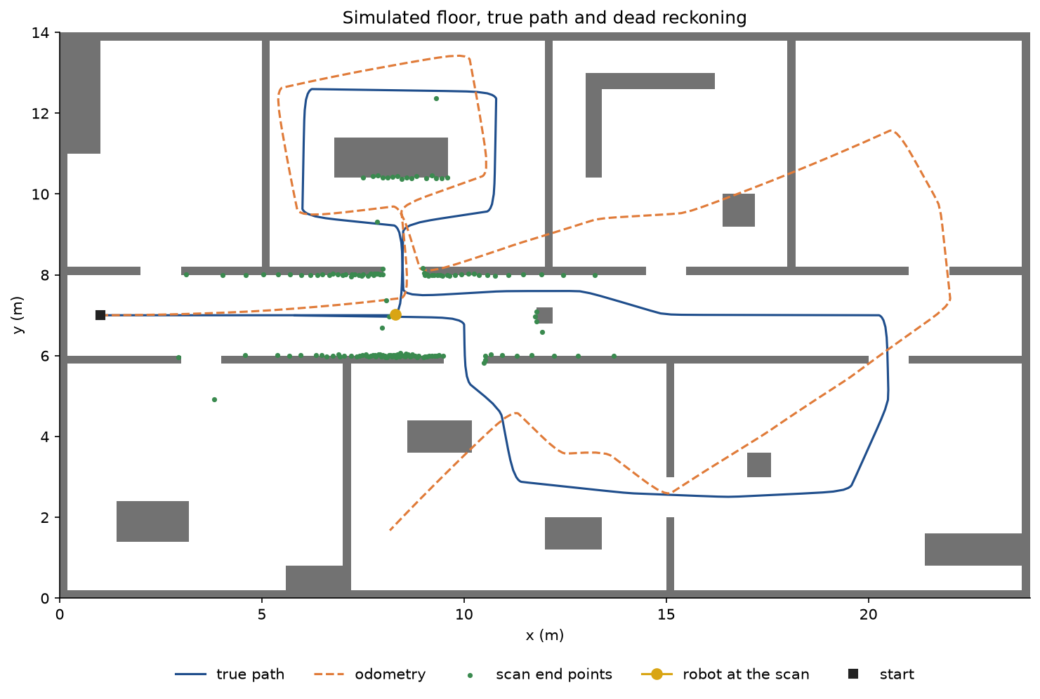
The dashed odometry path starts on the true path and drifts away with every turn; after the tour it is almost six metres off, which is why localization against the map is needed at all.

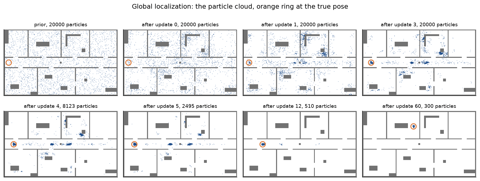
In global localization the first scans leave clusters in several rooms and along the corridor, where a stretch of featureless wall looks the same at many places. The cloud collapses onto the true pose when the robot passes the first door gaps, and KLD-sampling shrinks it from 20,000 particles to a few hundred.

After the kidnapping, the augmented filter keeps the old cluster in the corridor for a few updates while random particles spread over the floor. The ones that land in the north room fit the scans, take over at resampling, and the count falls back once the fast average has caught up with the slow one.

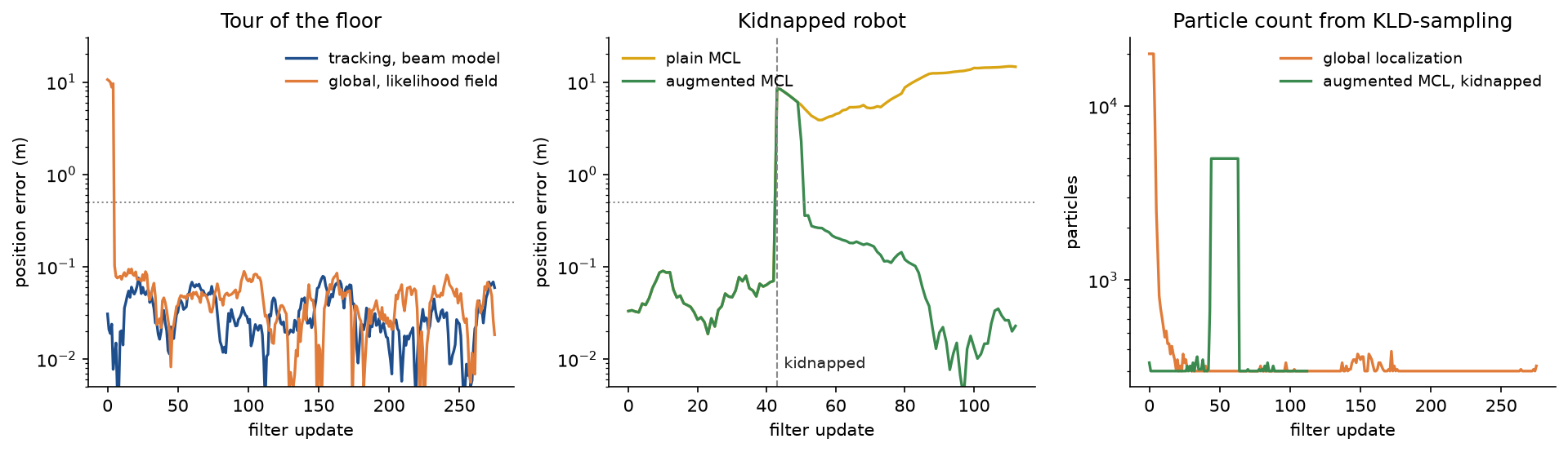
The left panel shows global localization joining the tracking filter's error level after five updates. In the middle panel plain MCL never comes back below the dotted 0.5 m line, while augmented MCL does; the right panel shows the particle count falling after global localization and jumping to its maximum while augmented MCL injects random particles.

The notebook localization.ipynb is a guided tour in the order of this page: the corridor, the motion model, ray casting, both sensor models, the five-particle step, the recovery and KLD numbers, demonstrations of the pitfalls, the three experiments of the project and the Nav2 parameter file. The tests in tests check the worked examples value by value, the mathematical properties above, the simulated experiments and the agreement with SciPy, and run in under ten seconds:

python -m pytest robotics/localization

Everything is synthetic: the floor plan, the trajectories, the odometry errors and the laser scans are generated from fixed seeds, so nothing is downloaded and no licence is involved.

In practice

The AMCL node in ROS 2 Nav2

Nav2's amcl node implements the same algorithm and takes the same quantities as parameters. The defaults below are those documented for recent Nav2 releases; check them against the version you run. For each idea on this page, the list gives the Nav2 parameter, its default, the value used here, and how the two differ:

• Motion model: robot_model_type, default nav2_amcl::DifferentialMotionModel, the differential model here. nav2_amcl::OmniMotionModel serves holonomic bases and also uses alpha5.
• Noise α1 to α4: alpha1 to alpha4, default 0.2 each; here 0.1, 0.05, 0.05 and 0.02. They are variance coefficients as in the formulas above, in the same order.
• Update triggers: update_min_d and update_min_a, default 0.25 m and 0.2 rad, the same here. Standing still is not an update; otherwise the same scan would multiply into the weights again and again.
• Sensor model: laser_model_type, default likelihood_field; the beam model for tracking and the likelihood field otherwise here. likelihood_field_prob adds optional beam skipping.
• Beam subset: max_beams, default 60; 30 here, evenly spaced over the scan.
• Mixture weights: z_hit, z_short, z_max and z_rand, default 0.5, 0.05, 0.05 and 0.5; here 0.7, 0.15, 0.05 and 0.1 for the beam model and 0.9 and 0.1 for the likelihood field. The likelihood field uses only z_hit and z_rand, and Nav2's Gaussian has peak 1 rather than unit area, which shifts the balance between the two.
• σ hit: sigma_hit, default 0.2 m, the same here.
• λ short: lambda_short, default 0.1; 0.5 here. It affects the beam model only.
• z max: laser_max_range and laser_min_range, default 100.0 and -1.0; 6.0 here. The value -1.0 means the range reported by the scanner.
• d max: laser_likelihood_max_dist, default 2.0 m, the same here; the distance at which the likelihood field stops changing.
• Combining beams: no parameter. Nav2's beam and likelihood-field models score a particle by 1 + Σ p³, fixed in the code; this page uses the tempered product with γ = 0.05.
• Particle count: min_particles and max_particles, default 500 and 2000; here 500 fixed for tracking, 300 to 20,000 for global localization and 300 to 5,000 for the kidnapping. The default maximum is too small for global localization on large maps.
• KLD ε: pf_err, default 0.05, the same here.
• KLD quantile: pf_z, default 0.99; 2.3263 here. It is the quantile itself, not a probability; see Pitfalls.
• Resampling: resample_interval, default 1. Nav2 has no effective-sample-size test; this page resamples below half the particle count for tracking and at every update otherwise.
• Recovery: recovery_alpha_slow and recovery_alpha_fast, default 0.0 and 0.0, which switches recovery off; 0.02 and 0.2 here. Nav2 suggests 0.001 and 0.1, and good values depend on how often the filter updates.
• Initial pose: set_initial_pose, initial_pose and the topic initialpose, default false; a Gaussian around the start here. The covariance sent on initialpose sets the spread of the first cloud.
• Global localization: the service reinitialize_global_localization, which spreads the particles over the free space of the map like uniform_state.
• Output: the topics amcl_pose and particle_cloud, which correspond to cluster_estimate and the particle set; amcl_pose carries the covariance of the heaviest cluster.

nav2_amcl_parameters writes a localizer in this vocabulary, and examples/library_equivalents.py prints the global localizer and the recovering localizer of the project that way. ROS 2 parameters are typed, and a value written as 6 for a parameter declared as a double is rejected, so format_parameters always writes floats with a decimal point:

from localization import (
    LikelihoodFieldModel,
    LikelihoodFieldSensor,
    MonteCarloLocalizer,
    floor_plan,
    format_parameters,
    nav2_amcl_parameters,
)

grid = floor_plan()
sensor = LikelihoodFieldSensor(grid, LikelihoodFieldModel())
localizer = MonteCarloLocalizer(grid, sensor, min_particles=300, max_particles=20000)
print(format_parameters(nav2_amcl_parameters(localizer)))

Cross-checks against libraries

There is no NumPy or SciPy particle filter to compare against, but two building blocks have library equivalents. distance_field agrees with scipy.ndimage.distance_transform_edt(~occupied, sampling=r) to within 10⁻¹⁵ m on the whole floor plan, and the particle count of kld_bound agrees with the count from the exact chi-square quantile scipy.stats.chi2.ppf to within 1 % for k from 5 to 1000. Both are tested in tests/test_comparisons.py and skipped when SciPy is not installed. Without SciPy, the 99th percentile of a million draws from NumPy's chi-square sampler agrees with the approximation to within 0.3 % for k from 2 to 200.

When to use which:

• A histogram filter for small, discrete problems, or where the whole distribution must be inspected; it is exact up to the grid.
• An extended Kalman filter for tracking with a good initial pose and a unimodal belief, for example against known landmarks. It is cheap and smooth but cannot hold two hypotheses, so it cannot do global localization.
• Monte Carlo localization when the belief can have several modes: global localization, symmetric buildings, recovery from failures. On a ROS 2 robot that means Nav2's AMCL; the from-scratch version is for understanding what its parameters do and for experiments the node does not allow.
• Scan matching against the map, or a graph-based localizer, when the map is large or three-dimensional and an initial guess is available; these give more precise poses but no multimodal belief. SLAM builds the maps that all of these localize against, and Navigation consumes the pose they produce.

Pitfalls

Every demonstration below is printed by examples/common_mistakes.py and shown again in the notebook's section "Pitfalls in code".

• Taking the mean of a cloud with several modes. The weighted mean of two hypotheses is a pose neither of them supports. Two clusters on either side of the wall between two south rooms, holding 0.55 and 0.45 of the weight, have their mean at (7.01, 3.00), inside the wall; the heaviest-cluster estimate stays at (6.20, 3.01). Treat the covariance as meaningful only when one cluster holds most of the weight.
• Averaging headings arithmetically. Particles at 175 and -175 degrees both point almost due west, but their arithmetic mean is 0 degrees, due east; the circular mean gives 180 degrees. The same applies to the covariance: angular deviations must be wrapped before they are squared.
• Multinomial resampling, and resampling too often. Resampling equal weights should change nothing. Low-variance resampling keeps all 1000 particles; multinomial resampling keeps 635 distinct ones after one round, 165 after 10 and 36 after 50. Resampling at every update when the weights carry little information wears the cloud down in the same way, which is what the effective-sample-size test prevents. In descriptions of low-variance resampling, check that the offset is drawn from [0, 1/M), not from [0, 1): with the wider range, pointers run past the end of the cumulative weights.
• Moving particles by the odometry displacement in the world frame. Adding the odometry's displacement to every particle is correct only for particles that share the odometry heading. One metre of forward motion moves a north-facing particle at (2, 2) to (3, 2) under that rule, sideways, instead of to (2, 3). Decompose the motion into rotation, translation and rotation and apply it in each particle's own frame.
• Pure rotations and reversing. Turning on the spot with 3.6 mm of position jitter gives a first rotation of -0.588 rad from the angle of the jitter, and with it a rotation standard deviation of 0.186 rad instead of 0.001 rad. Reversing 0.2 m decomposes into two half turns, which without folding gives a rotation standard deviation of 0.994 rad instead of 0.045 rad. tests/test_motion.py checks both guards.
• Reading pf_z as a probability. KLD-sampling needs the quantile z of 1 - δ, and Nav2's pf_z is that quantile. Its default of 0.99 is therefore δ = 0.161, a confidence of about 84 %, not 99 %. For 50 occupied bins it asks for 588 particles where 99 % confidence needs 750; set pf_z to 2.326 for the latter. Explanations that call the default "99 % confidence" repeat the misreading.
• Trusting the independence of beams. Multiplying 30 beam likelihoods as if they were independent makes the first scan of a global localization keep only the few particles that happen to fit best, and if none of them is near the true pose there is nothing left to recover with. On six simulated runs, the raw product localized the robot in 1 run after 60 updates; the product raised to γ = 0.05 localized it in all 6. Fewer beams, a larger σ hit and tempering all help; so do more particles at the start.
• Particle deprivation. A filter can only find the robot where it has particles. Plain MCL after the kidnapping keeps its cloud in the corridor and ends 14.62 m from the robot, while augmented MCL recovers in 8 updates, as the project shows and tests/test_runs.py checks. Motion noise set too small has the same effect on a smaller scale: the cloud cannot follow real slip. Choose the α values to cover the worst slip you expect, and switch on recovery for any robot that can be moved by hand.
• Multiplying densities instead of adding log densities. Thirty densities of order 10⁻³ multiply to 10⁻⁹⁰, and 400 such beams underflow double precision to exactly zero for every particle, while the sum of their logarithms is an ordinary number, about -2763. Sum log-likelihoods and subtract the largest before exponentiating, as normalize_log_weights does: log weights of -1000, -1001 and minus infinity become 0.7311, 0.2689 and 0.
• Dropping the truncation factor of the hit component. Near the end of the range half of the Gaussian lies beyond z max, so the factor is 2 when z* = z max: a reading of 5.9 m from a wall at 6.0 m has a hit density of 3.5207, not 1.7603. Leaving the factor out makes walls near the range limit look less informative than they are. Nav2's beam model omits it too, along with the normalization of its Gaussian, so its densities are scores rather than probabilities.
• Marching along a ray with a fixed step. Sampling a ray every 0.25 m from x = 0 never looks at a wall cell that covers [0.30, 0.40), so the beam passes through it and reports the maximum range of 1.5 m, where the cell traversal stops at 0.30 m. The traversal visits every cell the ray crosses and agrees with marching in steps of 0.1 mm to within 0.1 mm.
• Mixing up rows and columns of the map. An occupancy grid stored as an image has rows along y and columns along x, often with row 0 at the top. Indexing occupied[x, y] transposes the map and ray casting silently looks at the wrong cells: in the worked example's room, the forward range from (2.5, 2.0) becomes 1.50 m instead of 2.50 m. A quick test is a ray cast in a rectangular room whose distances are known, as in tests/test_ray_casting.py.

Further reading

• S. Thrun, W. Burgard and D. Fox, Probabilistic Robotics, MIT Press, 2005. Chapters 2, 4, 5, 6 and 8 cover the Bayes filter, histogram and particle filters, motion and measurement models, and Markov and Monte Carlo localization, including augmented MCL and KLD-sampling.
• F. Dellaert, D. Fox, W. Burgard and S. Thrun, "Monte Carlo localization for mobile robots", Proceedings of the IEEE International Conference on Robotics and Automation, 1999.
• D. Fox, W. Burgard, F. Dellaert and S. Thrun, "Monte Carlo localization: efficient position estimation for mobile robots", Proceedings of the National Conference on Artificial Intelligence (AAAI), 1999.
• D. Fox, "Adapting the sample size in particle filters through KLD-sampling", The International Journal of Robotics Research 22(12), 985-1003, 2003.
• N. J. Gordon, D. J. Salmond and A. F. M. Smith, "Novel approach to nonlinear/non-Gaussian Bayesian state estimation", IEE Proceedings F 140(2), 107-113, 1993. The bootstrap particle filter.
• A. Kong, J. S. Liu and W. H. Wong, "Sequential imputations and Bayesian missing data problems", Journal of the American Statistical Association 89(425), 278-288, 1994. The effective sample size.
• R. Douc, O. Cappé and E. Moulines, "Comparison of resampling schemes for particle filtering", Proceedings of the International Symposium on Image and Signal Processing and Analysis, 2005.
• W. Burgard, D. Fox, D. Hennig and T. Schmidt, "Estimating the absolute position of a mobile robot using position probability grids", Proceedings of the National Conference on Artificial Intelligence (AAAI), 1996. Grid-based Markov localization.
• J. Amanatides and A. Woo, "A fast voxel traversal algorithm for ray tracing", Eurographics, 1987.
• P. F. Felzenszwalb and D. P. Huttenlocher, "Distance transforms of sampled functions", Theory of Computing 8, 415-428, 2012.
• E. B. Wilson and M. M. Hilferty, "The distribution of chi-square", Proceedings of the National Academy of Sciences 17(12), 684-688, 1931.
• S. Macenski, F. Martín, R. White and J. Ginés Clavero, "The Marathon 2: a navigation system", Proceedings of the IEEE/RSJ International Conference on Intelligent Robots and Systems, 2020. The design of Nav2; its AMCL configuration guide lists every parameter discussed above.