Convolutional networks

A dense layer on a 128 × 128 colour image needs 49,152 weights for every unit it feeds, treats a pixel in the top-left corner as unrelated to its neighbour, and has to learn the same edge detector again at every position. A convolutional layer instead slides one small kernel across the whole image, so it has a handful of weights, keeps the spatial layout and finds a pattern wherever it occurs. This page works through the arithmetic that decides what such a network costs and what it sees: cross-correlation against true convolution on a 5 × 5 image by hand, output sizes under padding, stride and dilation, receptive fields, parameter and FLOP counts for standard, grouped, depthwise and depthwise separable layers, pooling, and the backward pass of a convolution. It implements convolution twice in NumPy, checks both against PyTorch, and trains a LeNet-style network on Fashion-MNIST. Afterwards you will be able to predict the shape, parameter count, multiply-accumulate count and receptive field of any convolutional layer on paper, see where a network's parameters and compute actually go, verify that a supposedly depthwise block really is one, and write and check a convolution's backward pass yourself. It builds on Backpropagation.

To run the code in this topic, install the base group, the deep group for PyTorch, and the ml group for the small digits set that the sample project falls back on when Fashion-MNIST has not been downloaded.

Intuition

Three ideas turn a dense layer into a convolutional one.

• Local connectivity. Each output value looks at a small window of the input, for example 3 × 3 pixels, because in images the pixels that matter together sit together.
• Weight sharing. The same kernel is used at every position. A detector learned in one place works everywhere, and the number of weights no longer depends on the size of the image.
• Channels. A layer holds many kernels, and each kernel looks through all channels of its input at once, so a layer turns Cin feature maps into Cout new ones.

A consequence of weight sharing is translation equivariance: shift the input and the feature maps shift with it. A single layer sees only a small window, but stacking layers grows the region each unit depends on, its receptive field, and pooling or striding halves the resolution so that later layers cover large regions cheaply. A classifier ends with a head that turns the last feature maps into class scores, either by flattening them into a dense layer or by averaging each map to a single number first.

The diagram shows the network the sample project trains on 28 × 28 grey images, with the shape of each layer's output as channels × height × width and its parameter count. Even in this small network the first dense layer holds 78 % of the 61,706 parameters, while the two convolutions do 86 % of the arithmetic. The two budgets are spent in different places, and this page shows how to count both.

How it works

Notation

Layers follow the notation of Backpropagation: layer l turns the activations a of layer l - 1 into net inputs z and activations a = f(z), and its error δ is the derivative of the cost C with respect to z. In a convolutional layer these are stacks of two-dimensional maps.

• Channel k of the layer's input is a map of H × W pixels, for k from 1 to Cin. Output channel j has a net-input map and an activation map of H′ × W′ pixels, for j from 1 to Cout.
• The kernels W have the shape Cout × Cin/g × Kh × Kw, the layout of torch.nn.Conv2d.weight. The kernel to output channel j from input channel k is a Kh × Kw map, "to j from k" as in the dense case, and each output channel has one bias b.
• P, S and D are the padding, stride and dilation, and g is the number of groups, with g = 1 for a standard convolution.
• X ⋆ K is the cross-correlation and X ∗ K the convolution of a map X with a kernel K, and X[p, q] is the entry in row p and column q, counted from 0.

The formula images write the layer as a superscript in parentheses; in the text and the code W, a, z and δ always belong to the layer under discussion. Mini-batches are four-dimensional arrays of shape N × C × H × W with one example per leading index, the layout of PyTorch, which plays the role of one example per row in the dense case.

Convolution and cross-correlation

For a map X and a kernel K of Kh × Kw entries, the cross-correlation slides the kernel across the map and takes a dot product at every position where it fits:

Convolution in the mathematical sense runs the kernel index backwards. Restricted to the positions where the kernel fits and counted from zero, it reads the first line below; substituting Kh - 1 - u for u and Kw - 1 - v for v turns it into a cross-correlation with the rotated kernel K̃:

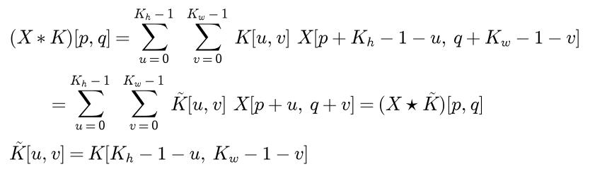
So convolution is cross-correlation with the kernel rotated by 180 degrees. Both are linear in X and in K, and both are translation equivariant: shifting X shifts the output by the same amount. Convolution also has algebraic properties cross-correlation lacks. It is commutative, X ∗ K = K ∗ X when both are evaluated in full (at every position where the two overlap at all), and associative, so two linear filters applied in turn equal one larger filter, the convolution of the two kernels. Cross-correlation is neither: in full mode K ⋆ X is X ⋆ K rotated by 180 degrees.

Deep-learning libraries compute cross-correlation and call it convolution. For learned kernels the difference is irrelevant, since a network trained with one operation simply learns the rotated kernels with the other. It matters when a kernel is fixed (an asymmetric edge or motion filter gives the opposite sign or a mirrored response), when results are compared across libraries (np.convolve and scipy.signal.convolve2d flip the kernel, torch.nn.functional.conv2d does not), and in the backward pass below, where a true convolution appears. Convolution and filtering treats fixed kernels in detail.

Output size: padding, stride and dilation

Three settings change where the kernel is placed along each axis.

• Padding P adds P zeros on both sides, so the padded length is H + 2P.
• Dilation D spreads the kernel entries D pixels apart. A kernel of K taps then spans D(K - 1) + 1 pixels while keeping K weights.
• Stride S moves the kernel S pixels at a time, so windows start at 0, S, 2S and so on.

Window i starts at pixel iS and ends at iS + D(K - 1), and it fits as long as that last pixel exists. The largest such i is a floor, and counting from i = 0 gives the output size:

The same holds for the width. Two consequences follow.

• At stride 1 the size is kept when 2P = D(K - 1), which needs an odd span: P = 1 for K = 3, P = 2 for K = 5, and P = 2 for K = 3 with D = 2. An even kernel cannot be padded symmetrically to keep the size.
• When S does not divide H + 2P - D(K - 1) - 1, the floor discards the remainder, and that many pixels at the far end are never read. A 3 × 3 kernel at stride 2 on a 28 × 28 map gives 13 × 13 outputs and ignores the last row and column.

Pooling layers place their windows the same way, with D = 1 and usually K = S = 2.

Receptive fields

The receptive field of a unit is the set of input pixels that can affect it. Track two numbers through the layers: the side r of the field of a unit in layer l, and the jump j, the distance in input pixels between neighbouring units of layer l. The input has r = 1 and j = 1. A unit of layer l reads K units of layer l - 1 placed D apart; those units are j pixels apart in the input and each sees r pixels, so the field grows by D(K - 1) times the old jump, and a stride multiplies the jump. The second line tracks the centre c of the first unit's field, which starts at 0, the centre of the first pixel:

Three facts follow.

• n stacked 3 × 3 layers at stride 1 see 2n + 1 pixels. Three of them see 7 × 7 with 3 × 9 = 27 weights per channel pair, against 49 for one 7 × 7 layer, and add two non-linearities on the way.
• Every stride or pooling layer multiplies the jump, so the layers after it grow the field faster for the same kernel size.
• Dilations 1, 2, 4 and so on up to 2 to the power n - 1 give a field of 2 to the power n + 1, minus 1: it grows exponentially with depth at a constant number of weights per layer.

The field is not uniform. A pixel near its centre reaches the unit through many more paths than a pixel at its edge, so the effective receptive field is concentrated in the middle. Sending a gradient of 1 back from one unit through kernels of all ones counts these paths:

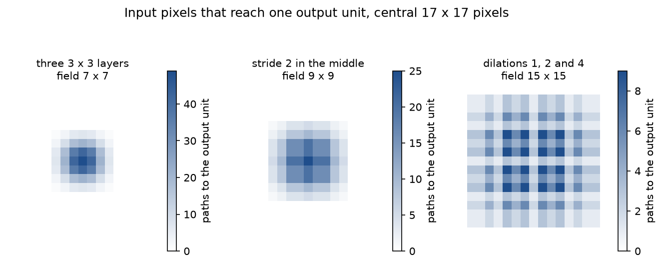
All three fields have exactly the predicted size, and in all three a corner pixel reaches the unit through a single path. The dilated stack covers by far the largest region with the same 27 weights per channel pair, but it spreads its paths unevenly in a checkered pattern, which is one reason dilated layers are usually mixed with plain ones.

Multi-channel convolution and groups

A convolutional layer computes, for each output channel j and position (p, q), a sum over every input channel, every kernel offset and the window that padding, stride and dilation select; entries outside the map are zero:

At stride 1, without padding or dilation, this is a sum of cross-correlations, one per input channel:

Every kernel of output channel j spans the full input depth, and its responses on the separate channels are added. The layer is the dense layer z = W a + b with each weight replaced by a small kernel and each product by a cross-correlation.

Groups restrict which input channels an output channel reads. With g groups the input channels are split into g consecutive blocks of Cin/g and the output channels into g blocks of Cout/g, and output channel j sums only over the input block with the same index as its own block. Three special cases have names.

• Standard convolution: g = 1.
• Depthwise convolution: g = Cin and Cout = m Cin for a channel multiplier m, usually 1. Output channel j reads only input channel j/m rounded down, counting from 0.
• Pointwise convolution: Kh = Kw = 1. It is the dense layer applied at every pixel, mixing channels but not positions.

A depthwise separable convolution is a depthwise layer followed by a pointwise one: the first filters each channel spatially on its own, the second mixes channels.

Together the pair represents exactly the standard convolutions whose kernel tensor factors into a pointwise weight times a per-channel spatial kernel, a rank restriction that buys a large saving:

A standard layer has Cout Cin Kh Kw free kernel entries; the factored form has only Cout Cin + Cin Kh Kw, which is where the saving counted next comes from.

Parameter and FLOP budgets

Each output value is a dot product of length (Cin/g) Kh Kw plus a bias, and there are H′ W′ Cout output values. Counting one multiply-accumulate (MAC) per product term, and ignoring the bias additions and activations, which cost one operation per output value, gives the parameters N and MACs M of each kind of layer:

Pooling has no parameters and, counted in MACs, no arithmetic. A FLOP count usually counts the multiply and the add separately, so FLOPs are twice the MACs. Grouping divides both budgets by exactly g. A depthwise separable pair on the same output grid has the parameters and MACs of its two layers added, and without biases it costs, relative to the standard convolution it replaces:

The parameter ratio is the same expression. For 3 × 3 kernels and wide layers it approaches 1/9; narrow layers save less, and with 8 output channels the ratio is 1/8 + 1/9 = 0.2361.

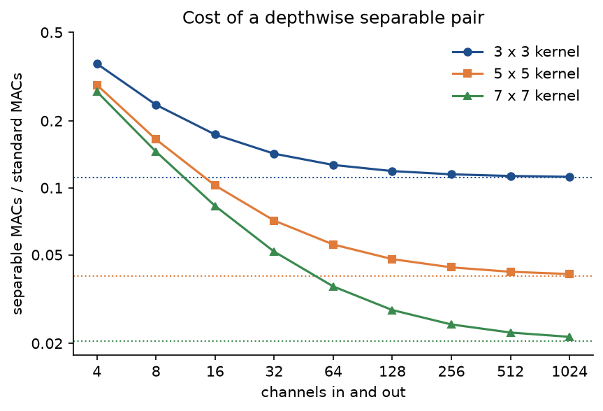
The plot shows that the saving depends on the width as much as on the kernel: at 16 channels a 3 × 3 separable pair still costs 17 % of the standard layer, and only beyond a few hundred channels does it come close to the floor of one ninth.

Pooling and global average pooling

Pooling replaces each window of a single channel by one number, its maximum (max pooling) or its mean (average pooling), with windows placed by the output-size formula. It has no parameters, works on each channel separately, shrinks the maps that later layers must process, multiplies the jump and with it the growth of the receptive field, and makes the output change less under shifts of a pixel or two. A strided convolution does the same downsampling with learned weights.

Global average pooling averages each channel over all positions, turning C maps of any size into a vector of C numbers:

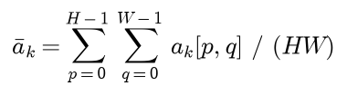
It equals average pooling with a window the size of the whole map, and because it ignores where a response occurred it is exactly invariant to shifts that keep the object inside the map. The backward passes follow from the derivatives of the maximum and the mean. Max pooling passes each output gradient to the single input that won its window and gives the others zero; average pooling spreads it equally, 1/(Kh Kw) to each input of the window; and global average pooling gives every pixel of a channel the share 1/(HW) of its gradient.

Where the parameters live

Suppose the last convolutional block leaves a map of C × H × W. Flattening it into a dense layer of n units costs a number of parameters that grows with the image area, while a global average pooling head that feeds the class scores directly costs C weights per class:

The convolutional layers themselves cost Cout Cin Kh Kw + Cout each, independent of the image size. For large images the first dense layer therefore holds almost all parameters: in the six-class network of the worked example below it holds 99.15 % of them. Global average pooling also lets the network accept any input size and removes what is often the largest source of overfitting in a small convolutional network.

Compute is distributed the other way round. A convolution repeats its dot products at every output position, so its MACs are its weight count times H′W′, while a dense layer uses each weight exactly once per example. The convolutions dominate the arithmetic and the first dense layer dominates the memory, which is why both budgets have to be counted per layer.

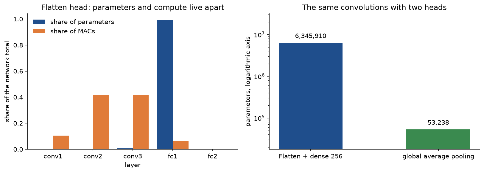
The left panel makes the split visible: the blue bars, the parameters, sit almost entirely on fc1, and the orange bars, the MACs, on the convolutions. The right panel shows what swapping the head does to the total.

Backpropagation through a convolution

Take one channel at stride 1 without padding, with a single kernel w, bias b, input map a and error map δ:

Each parameter and each input pixel reaches the cost through several net inputs, so the chain rule sums over them, exactly as in the derivation of the equations B2 to B4 for dense layers. The bias enters every net input with coefficient 1, which gives the convolutional form of B3:

The weight at offset (u, v) multiplies the input pixel at (p + u, q + v) in every net input, which gives the convolutional form of B4:

The kernel gradient is the cross-correlation of the layer's input with its error map. Weight sharing is why it is a sum: one weight serves every position, so its gradient collects the contributions of all of them, as the batch sum collects the contributions of all examples. The input pixel at (i, j) appears in the net input at (p, q) with coefficient w[i - p, j - q] whenever that offset lies inside the kernel, which gives the convolutional form of B2:

This is a true convolution, evaluated in full: equivalently, pad the error with K - 1 zeros on every side and cross-correlate it with the rotated kernel. Read as a scatter, each error entry stamps a copy of the kernel, scaled by that entry, onto the input gradient at its own offset. Multiplying by the derivative of the previous layer's activation then gives that layer's error, as in B2. With several channels each output channel adds its share:

The last sum runs over the output channels that read channel k, the counterpart of the transpose in B2. Over a mini-batch the kernel and bias gradients add the contributions of all examples; if the cost is a mean, its factor 1/m is already inside δ. A stride S spreads the error entries S pixels apart before the full convolution, and padding crops P pixels from each side of the input gradient.

The im2col view makes all of this one matrix product. Copy every receptive-field patch of the input into a column: the patch matrix A has Cin Kh Kw rows, one per channel and kernel offset, and H′W′ columns, one per output position. Reshape the kernels into a matrix Wmat of Cout rows and Cin Kh Kw columns, and the outputs into Z of Cout rows and H′W′ columns. With Δ the error reshaped like Z:

The diagram draws the same matrices as a data flow, the forward pass in solid blue and the backward pass in dashed orange.

A convolution is a dense layer applied to the patch matrix, and its backward pass is the dense backward pass followed by col2im: every entry of the patch gradient is added back to the pixel it was copied from, so overlapping patches accumulate. im2col copies and col2im adds; as linear maps they are each other's transpose.

Verifying that a layer is depthwise

The channel connectivity of a layer is the yes-or-no matrix M with one row per output channel and one column per input channel, whose entry is 1 when output channel j depends on input channel k. A standard convolution has M full of ones, g groups give g diagonal blocks, and a depthwise layer has exactly one 1 per row. Because a convolution is affine, its output minus its output at zero input is linear in the input, so an input that is random in channel k and zero elsewhere changes exactly the output channels in column k of M; random values make an accidental zero response a probability-zero event. Three checks, from cheapest to strongest:

1. The configuration: groups == in_channels and a weight of shape (m Cin, 1, Kh, Kw).
2. The parameter count against the depthwise formula.
3. The measured M, which tests the computation that actually runs rather than its name or its configuration.

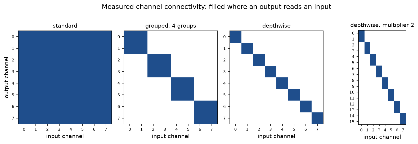
The four patterns are exactly the group masks the configurations promise, which is what the measurement is for: it would show a full square for a layer that was meant to be depthwise but was built without its groups.

Worked example

A 5 × 5 image X and a 3 × 3 kernel K with bias 0, small integers so that every value is exact. The rows of X are (1, 0, 2, 1, 0), (0, 3, 1, 0, 2), (2, 1, 0, 3, 1), (1, 0, 2, 1, 3) and (0, 2, 1, 0, 1). The rows of K are (1, 2, 0), (0, 1, -1) and (-1, 0, 1). All results are integers except two averages in the pooling step, which are exact at the decimals shown.

Cross-correlation and convolution

The kernel fits in 5 - 3 + 1 = 3 positions along each axis. For output (0, 1) it covers rows 0 to 2 and columns 1 to 3 of X, whose rows there are (0, 2, 1), (3, 1, 0) and (1, 0, 3):

• 1 × 0 + 2 × 2 + 0 × 1 = 4 from the first row,
• 0 × 3 + 1 × 1 + (-1) × 0 = 1 from the second,
• (-1) × 1 + 0 × 0 + 1 × 3 = 2 from the third,

so the output is 4 + 1 + 2 = 7. Repeating this at all nine positions gives X ⋆ K with rows (1, 7, 3), (8, 3, 4) and (3, 0, 4).

The true convolution uses the kernel rotated by 180 degrees, K̃, whose rows are (1, 0, -1), (-1, 1, 0) and (0, 2, 1). Cross-correlating with it gives X ∗ K with rows (4, 0, 8), (0, 7, 7) and (6, 2, -1). At output (1, 0) the window has rows (0, 3, 1), (2, 1, 0) and (1, 0, 2); with K it gives 0 + 6 + 0 + 0 + 1 + 0 - 1 + 0 + 2 = 8, with K̃ it gives 0 + 0 - 1 - 2 + 1 + 0 + 0 + 0 + 2 = 0. The two operations agree only for kernels that are symmetric under the rotation.

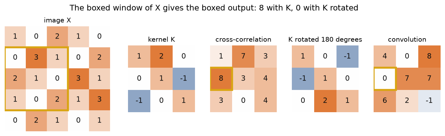
The figure follows one window through both operations: the same nine pixels give 8 with the kernel as written and 0 with the rotated one.

Padding, stride and dilation

With padding 1 and stride 2 the output has (5 + 2 - 2 - 1)/2 + 1 = 3 entries per axis. Window (i, j) covers padded rows 2i to 2i + 2, which are original rows 2i - 1 to 2i + 1. At (0, 0) only the bottom-right 2 × 2 corner of the kernel lands on the image: 1 × 1 + (-1) × 0 + 0 × 0 + 1 × 3 = 4. All nine outputs form the rows (4, -2, 0), (1, 3, 4) and (0, 5, 8). The centre entry covers original rows and columns 1 to 3, the same window as entry (1, 1) of X ⋆ K, and both equal 3.

With dilation 2 and no padding the kernel spans 2 × (3 - 1) + 1 = 5 pixels, so it fits once and reads every other pixel, X[2u, 2v], whose rows are (1, 2, 0), (2, 0, 1) and (0, 1, 1):

• 1 × 1 + 2 × 2 + 0 × 0 = 5,
• 0 × 2 + 1 × 0 + (-1) × 1 = -1,
• (-1) × 0 + 0 × 1 + 1 × 1 = 1,

which adds up to 5.

Pooling

A 2 × 2 window with stride 2 fits (5 - 2)/2 + 1 = 2 times per axis, rounded down, and the remainder of 1 means that row 4 and column 4 of X are never read. The four windows hold (1, 0, 0, 3), (2, 1, 1, 0), (2, 1, 1, 0) and (0, 3, 2, 1), so max pooling gives the rows (3, 2) and (2, 3), and average pooling gives the rows (1, 1) and (1, 1.5). Global average pooling of X ⋆ K gives 33/9 = 3.6667.

Backward pass

Suppose the layers above hand back the error δ with rows (1, 0, -1), (0, 2, 0) and (-1, 0, 1) for the output X ⋆ K, which is what the cost C equal to the sum of δ times X ⋆ K, entry by entry, would produce. The bias gradient is the sum of the error, 1 - 1 + 2 - 1 + 1 = 2.

The kernel gradient is X ⋆ δ. Only five entries of δ are non-zero, so the gradient at offset (u, v) is X[u, v] - X[u, v + 2] + 2X[u + 1, v + 1] - X[u + 2, v] + X[u + 2, v + 2]. For (u, v) = (0, 0) this is 1 - 2 + 6 - 2 + 0 = 3, and in full the kernel gradient has the rows (3, 3, 3), (2, 4, 6) and (3, 0, 1).

The input gradient is the full convolution of δ with K: five copies of K, scaled by 1, -1, 2, -1 and 1, stamped at offsets (0, 0), (0, 2), (1, 1), (2, 0) and (2, 2) and added. At the centre all five copies overlap: K[2, 2] - K[2, 0] + 2K[1, 1] - K[0, 2] + K[0, 0] = 1 + 1 + 2 - 0 + 1 = 5. In full the input gradient has the rows:

• (1, 2, -1, -2, 0)
• (0, 3, 3, -1, 1)
• (-2, -2, 5, 0, -1)
• (0, -3, 1, 3, -1)
• (1, 0, -2, 0, 1)

PyTorch's autograd returns the same three gradients for torch.nn.functional.conv2d.

Receptive field of the LeNet-style network

Apply the recurrence to the network of the first diagram, starting with a field of 1 and a jump of 1:

• conv1, a 5 × 5 kernel at stride 1 with padding 2: field 1 + 4 × 1 = 5, jump 1.
• pool1, a 2 × 2 window at stride 2: field 5 + 1 × 1 = 6, jump 2.
• conv2, a 5 × 5 kernel at stride 1: field 6 + 4 × 2 = 14, jump 2.
• pool2, a 2 × 2 window at stride 2: field 14 + 1 × 2 = 16, jump 4.

Each of the 400 inputs of the first dense layer sees a 16 × 16 patch of the 28 × 28 image, and neighbouring ones are 4 pixels apart. The first of them is centred at 0 + 0 + 0.5 + 4 + 1 = 5.5, so its field spans pixels -2 to 13 and includes two rows and columns of padding.

Budget of one layer

A layer with 48 input channels, 96 output channels and 3 × 3 kernels on a 32 × 32 map, padded to keep the size, so H′W′ = 1,024:

• Standard: 96 × 48 × 9 + 96 = 41,568 parameters and 1,024 × 41,472 = 42,467,328 MACs.
• Grouped with g = 4: 96 × 12 × 9 + 96 = 10,464 parameters and 10,616,832 MACs, exactly 0.2500 of the standard layer.
• Depthwise: 48 × 9 + 48 = 480 parameters and 1,024 × 432 = 442,368 MACs, 0.0104 of the standard layer.
• Pointwise: 96 × 48 + 96 = 4,704 parameters and 1,024 × 4,608 = 4,718,592 MACs, 0.1111 of the standard layer.
• Depthwise separable: 480 + 4,704 = 5,184 parameters and 442,368 + 4,718,592 = 5,160,960 MACs, 0.1215 of the standard layer.

The last ratio is 1/96 + 1/9 = 0.0104 + 0.1111 = 0.1215, as the formula predicts. In FLOPs the standard layer costs 84,934,656. If the depthwise layer of the separable block is built without its groups, it becomes a standard 48-to-48 convolution with 48 × 48 × 9 + 48 = 20,784 parameters, and the block has 25,488: nearly five times the intended 5,184, yet still fewer than the 41,568 of the standard layer.

Budget of a network: Flatten against global average pooling

A six-class classifier for 3 × 128 × 128 images with three blocks of a 3 × 3 convolution (padding 1, ReLU) and 2 × 2 max pooling, with 24, 48 and 96 channels, leaves a 96 × 16 × 16 map. With Flatten and a dense layer of 256 units the layers cost:

• conv1, output 24 × 128 × 128: 672 parameters (0.01 %), 10,616,832 MACs (10.42 %).
• conv2, output 48 × 64 × 64: 10,416 parameters (0.16 %), 42,467,328 MACs (41.70 %).
• conv3, output 96 × 32 × 32: 41,568 parameters (0.66 %), 42,467,328 MACs (41.70 %).
• fc1, 256 units: 24,576 × 256 + 256 = 6,291,712 parameters (99.15 %), 6,291,456 MACs (6.18 %).
• fc2, 6 units: 1,542 parameters (0.02 %), 1,536 MACs (0.00 %).

In total 6,345,910 parameters and 101,844,480 MACs. The first dense layer holds 99.15 % of the parameters and does 6.18 % of the arithmetic. Replacing Flatten and both dense layers by global average pooling and one dense layer of 96 × 6 + 6 = 582 parameters leaves 53,238 parameters, 119 times fewer, and 95,552,064 MACs, 6 % fewer. The receptive field of the last pooled units is 22 pixels, so the head sees features of regions about a sixth of the image wide. Every number in this section is asserted by the tests in tests, mostly tests/test_trace.py, tests/test_costs.py, tests/test_budget.py and tests/test_receptive_field.py, and printed by examples/hand_calculation.py, examples/receptive_fields.py and examples/parameter_budgets.py.

The code

The package convolutional_networks is NumPy first, split into one module per idea. PyTorch is imported only inside the functions of comparisons.py and training.py, and scikit-learn only inside load_bundled_digits, so the from-scratch arithmetic works without either.

• arrays.py holds the Array and Size types and the shape checks as_image and as_tensor.
• correlation.py holds correlate2d and convolve2d, literal loops over output positions in valid or full mode, and flip, which rotates a kernel.
• geometry.py holds output_size, ignored_pixels, same_padding and conv_output_shape.
• receptive_field.py holds the recurrence (advance, receptive_fields) and gradient_footprint, which measures a field and counts its paths with the backward pass.
• convolution.py holds the two batched implementations, conv2d_direct and conv2d_im2col, with im2col and col2im; both handle padding, stride, dilation and groups, with different settings along the two axes.
• backward.py holds conv2d_backward, which returns the input, kernel and bias gradients.
• pooling.py holds max, average and global average pooling with the backward passes of the first two.
• costs.py holds conv_parameters, conv_macs, convolution_costs for the five kinds of layer and separable_cost_ratio.
• layers.py holds the layer specifications Conv, Pool, Flatten, GlobalAveragePool and Dense, and three networks: lenet_layers, digits_layers and image_classifier_layers.
• budget.py walks a specification with budget, one LayerBudget per layer, and prints it with format_budget.
• network.py runs a specification in NumPy with initialize_parameters, forward and forward_in_batches.
• connectivity.py measures channel connectivity and interprets it with group_mask, connectivity_groups and is_depthwise.
• trace.py holds the worked example and every value it produces, and problems.py the random convolution problems that the tests and comparisons share.
• idx.py, download.py and datasets.py parse the IDX format, fetch and verify Fashion-MNIST, load the bundled digits, split by class and standardize; metrics.py holds accuracy, the confusion matrix and its summaries.
• training.py trains a specification with PyTorch and keeps the best validation epoch; comparisons.py builds PyTorch models from specifications, copies weights back, and wraps autograd and the FLOP counter.
• pitfalls.py holds the small demonstrations of the Pitfalls section, and plotting.py and training_plots.py draw every figure in the handbook's four colours.

conv2d_direct evaluates the defining sum with one array operation per kernel offset rather than one per output value: for each offset it takes the shifted, strided slice of the padded input that this offset touches at every output position and multiplies it by the kernel entries of every channel pair. conv2d_im2col builds the patch matrix once and does one matrix product per group, and conv2d_backward is the dense backward pass on the same matrices, followed by col2im:

weight_gradient = np.matmul(delta, np.swapaxes(columns, 2, 3)).sum(axis=0)
column_gradient = np.matmul(np.swapaxes(matrix, 1, 2)[None], delta)
column_gradient = column_gradient.reshape(batch, in_channels * kh * kw, oh * ow)
input_gradient = col2im(column_gradient, x.shape, (kh, kw), stride, padding, dilation)

The examples and the project import the package, so install the repository first as described in the main README. The examples each demonstrate one idea and run in a few seconds at most from the repository root:

• examples/hand_calculation.py prints every value of the worked example in the order above and draws the worked-example figure.
• examples/receptive_fields.py applies the recurrence to the LeNet-style network, compares plain and dilated stacks, and measures three fields with the backward pass.
• examples/parameter_budgets.py prints the budgets of one layer, of the LeNet-style network and of the six-class network with both heads, and draws the two budget figures.
• examples/depthwise_check.py measures the channel connectivity of four PyTorch layers and catches a separable block built without its groups.
• examples/compare_with_pytorch.py checks both convolutions, their backward pass and pooling against PyTorch on seven configurations, and the budgets against PyTorch's parameter and FLOP counts.
• examples/common_mistakes.py demonstrates the mistakes listed under Pitfalls.

python computer-vision/convolutional-networks/examples/hand_calculation.py
python computer-vision/convolutional-networks/examples/receptive_fields.py
python computer-vision/convolutional-networks/examples/parameter_budgets.py
python computer-vision/convolutional-networks/examples/depthwise_check.py
python computer-vision/convolutional-networks/examples/compare_with_pytorch.py
python computer-vision/convolutional-networks/examples/common_mistakes.py

The sample project, project/fashion_classifier.py, applies everything to a real image classification task. It uses Fashion-MNIST when a verified copy is already in .data/convolutional-networks/ and otherwise falls back to the 8 × 8 digits that ship with scikit-learn, so the default run never touches the network; --download fetches Fashion-MNIST first. It splits one sixth of the training images off for validation, stratified by class, standardizes the pixels with statistics of the fitting images alone, prints the parameter, MAC and FLOP budget and receptive field of every layer and checks the totals against PyTorch, trains the LeNet-style network with Adam on one thread, keeps the epoch with the best validation accuracy, evaluates once on the test set, prints the recall of every class and the most frequent confusions, reruns the trained weights through the NumPy layers, and saves three figures. Options such as --dataset, --epochs, --batch-size, --learning-rate and --seed change the setup, and --figures sends the PNGs elsewhere so a custom run does not overwrite the ones shown here.

The order matters as much as the network: every choice, from the pixel statistics to the epoch, is made before the test set is touched.

python computer-vision/convolutional-networks/project/fashion_classifier.py --download
python computer-vision/convolutional-networks/project/fashion_classifier.py
python computer-vision/convolutional-networks/project/fashion_classifier.py --dataset digits

With Fashion-MNIST cached, the default run takes about half a minute on one CPU thread and stays near 1 GB of memory. The pixels of the 50,000 fitting images have mean 0.2859 and standard deviation 0.3530. Over six epochs of Adam with learning rate 0.002 and mini-batches of 128, validation accuracy goes 0.8316, 0.8763, 0.8856, 0.8738, 0.8903 and 0.8912, so the weights of epoch 6 are kept, while accuracy on the fitting images rises to 0.9105 and the validation loss is already lowest at epoch 5. On the 10,000 test images the network reaches an accuracy of 0.8834 with a test loss of 0.3164.

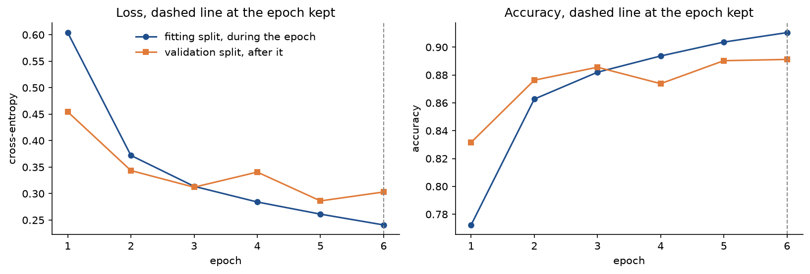
The fitting curves keep improving while the validation curves flatten and wobble after epoch 3, the usual first sign of overfitting; with more epochs the gap would widen.

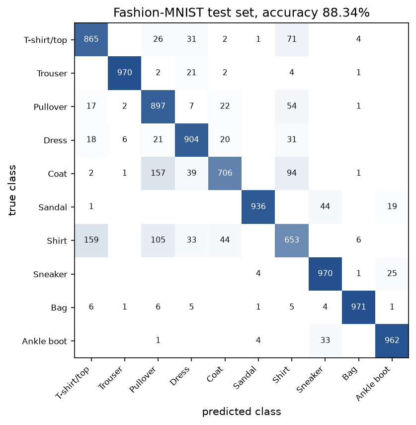
The errors concentrate among the upper-body garments. Shirt is recognized 65.30 % of the time, Coat 70.60 %, T-shirt/top 86.50 % and Pullover 89.70 %, against 97.10 % for Bag. The most frequent confusions are 159 shirts called T-shirts (71 the other way round), 157 coats called pullovers (22 the other way) and 105 shirts called pullovers (54 the other way).

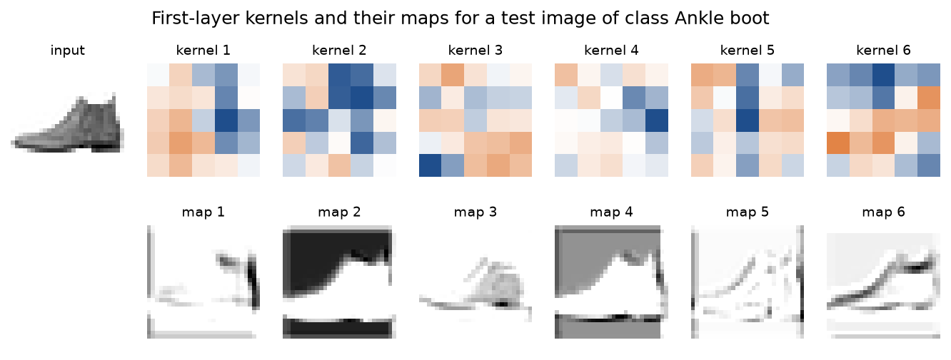
Several first-layer kernels have become oriented edge detectors that pick out the outline of the boot, while two respond mostly to the flat background around it. Finally the trained weights are copied into the NumPy layers: on all 10,000 test images the logits differ from PyTorch's by at most 6.7 × 10⁻⁶, the gap between single and double precision, and every predicted class is the same. Without the download the same command trains the smaller digits_layers network, 3,658 parameters, for 20 epochs on 1,199 of the 1,438 training digits in about two seconds, keeps epoch 11, and reaches a test accuracy of 0.9638 on 359 held-out digits.

The notebook convolutional_networks.ipynb is a guided tour in the order of this page: the worked example through trace_worked_example, both implementations against PyTorch, receptive fields measured with the backward pass, the layer and network budgets, the depthwise check, a demonstration of each pitfall, and a training run on whichever data set is available, rerun in NumPy. The tests in tests check the worked example value by value, the mathematical properties above and the agreement with PyTorch, and run in under ten seconds:

python -m pytest computer-vision/convolutional-networks

Data: Fashion-MNIST by Zalando Research, 70,000 grey 28 × 28 images of clothing in ten balanced classes, released under the MIT licence. fetch downloads the four gzip files on request from the dataset's repository on GitHub, falling back to the storage bucket it links to, checks each against the SHA-256 sum pinned in FASHION_MNIST_SHA256 (their MD5 sums match the ones the authors publish) before moving it into .data/convolutional-networks/ at the repository root, and the IDX header is validated before any array is read. The fallback is the optical recognition of handwritten digits data set from the UCI Machine Learning Repository, 1,797 images of 8 × 8 pixels, licensed CC BY 4.0 and shipped inside scikit-learn, so it needs no download. Nothing is committed.

In practice

In PyTorch a convolution is torch.nn.Conv2d(in_channels, out_channels, kernel_size, stride, padding, dilation, groups, bias) or the functional torch.nn.functional.conv2d, and its weight has our layout, (Cout, Cin/g, Kh, Kw). In double precision our direct and im2col implementations agree with it to within 10⁻¹⁴, forward and backward, on seven configurations that combine batches, groups, unequal strides, padding and dilation along the two axes, and the pooling layers agree to within 10⁻¹⁵ (examples/compare_with_pytorch.py, tests/test_backward.py, tests/test_pooling.py). Pooling is nn.MaxPool2d and nn.AvgPool2d, global average pooling is nn.AdaptiveAvgPool2d(1) followed by nn.Flatten(), and a depthwise separable pair is nn.Conv2d(c, c, k, padding=k // 2, groups=c) followed by nn.Conv2d(c, c_out, 1).

import torch
from torch.utils.flop_counter import FlopCounterMode

from convolutional_networks import budget, lenet_layers, to_torch, total_macs, total_parameters

layers = lenet_layers()
rows = budget(layers, (1, 28, 28))
model = to_torch(layers, (1, 28, 28))
with FlopCounterMode(display=False) as counter:
    model(torch.zeros(1, 1, 28, 28))
print(sum(p.numel() for p in model.parameters()), counter.get_total_flops())
print(total_parameters(rows), 2 * total_macs(rows))

Parameter counts from sum(p.numel() for p in model.parameters()) and FLOPs from torch.utils.flop_counter.FlopCounterMode, which counts two FLOPs per multiply-accumulate and leaves out the bias additions, agree exactly with budget and convolution_costs: 61,706 parameters and 833,040 FLOPs for the LeNet-style network, 6,345,910 and 203,688,960 for the six-class network with a Flatten head, and 53,238 and 191,104,128 with global average pooling.

When to use which:

• Use the from-scratch functions to learn the arithmetic, to check a hand calculation, and to reason about a layer's shape, cost and gradient before building it.
• Use torch.nn.Conv2d for anything that trains. Production libraries do not materialize im2col naively: cuDNN, oneDNN and XNNPACK choose per layer between implicit matrix products, Winograd transforms and FFTs, and fuse the bias and activation. A naive patch matrix costs memory: for 64 maps of 16 × 28 × 28 and a 3 × 3 kernel it takes 55.1 MiB against 6.1 MiB for the input, 9.0 times as much.
• Use budget or FlopCounterMode before training a new architecture, and look at the per-layer split, not just the totals.
• Prefer global average pooling over Flatten for the head unless the position of a feature in the image carries the label.
• Expect smaller wall-clock savings than MAC savings from depthwise separable blocks. A depthwise layer does very little arithmetic per byte of memory it reads, so on CPUs and GPUs it is limited by memory bandwidth, and the pointwise layer usually dominates the run time. Model compression returns to this on small devices.
• Set the number of CPU threads explicitly with torch.set_num_threads. The thread count changes the order of floating-point additions and therefore the trained weights, so the project and the notebook pin one thread and deterministic algorithms to make their outputs reproducible on any machine. On a busy machine, PyTorch's default of one thread per core competes with other processes and stalls at every synchronization point, which can make training many times slower than with a few threads.
• When a convolution is followed by batch normalization, build it with bias=False: the normalization subtracts the mean and would remove the bias again. Batch normalization adds 2C trainable parameters per layer and 2C running statistics, which are buffers, not parameters.

Pitfalls

• Calling cross-correlation convolution. The two differ by a 180-degree rotation of the kernel, so results differ for any asymmetric kernel. np.convolve([2, -1, 0.5, 3, 1], [1, 0, -2], "valid") gives (-3.5, 5, 0), while np.correlate and PyTorch's conv1d give (1, -7, -1.5) for the same inputs. Port a fixed kernel between libraries only after checking which operation each computes; examples/common_mistakes.py prints all of them.
• Trusting a hand-computed convolution table. Worked convolutions in tutorials and notes regularly contain arithmetic slips, and a table with a few wrong entries looks exactly as plausible as a correct one; a kernel applied unrotated where the text says convolution, or with rows and columns swapped, gives a different table that is just as believable. Recompute any table with two independent implementations before using it, as the worked-example tests do with correlate2d, conv2d_direct, conv2d_im2col and PyTorch.
• Off-by-one output sizes and pixels that are never read. The output-size formula has a floor, and frameworks apply it silently. A 3 × 3 kernel at stride 2 without padding on a 28 × 28 map gives 13 × 13 outputs and never reads the last row and column; overwriting them with 100 leaves the output identical (unread_pixels, printed by examples/common_mistakes.py). Choose sizes so that S divides H + 2P - D(K - 1) - 1, or pad. padding="same" in PyTorch is refused for strides above 1, and for an even kernel it has to pad one side more than the other.
• A depthwise block that is not depthwise. A separable block whose first layer was built without groups=in_channels still runs, still has the right output shape and still has fewer parameters than the standard convolution it replaces, because its middle width is Cin rather than Cout. For 48 to 96 channels with 3 × 3 kernels it has 25,488 parameters against 5,184 for the real block and 41,568 for the standard layer, so a saving appears and the bug goes unnoticed. Compare the parameter count with the formula and measure the connectivity, as examples/depthwise_check.py and the notebook section "Is the block really depthwise?" do.
• Judging a network's size by its convolutions. A Flatten head on a large final map can hold nearly all the parameters: 99.15 % in the worked example, 78 % even in the LeNet-style network. Count per layer with budget, and use global average pooling when the head is the problem.
• Confusing parameters, MACs and FLOPs. Parameters measure memory, MACs and FLOPs measure arithmetic, and the two are concentrated in different layers. FLOPs are twice the MACs, but papers and tools disagree on which of the two they call FLOPs, so a factor of exactly two between two published numbers is usually the unit: for the 48-to-96 layer the formula gives 42,467,328 MACs and FlopCounterMode reports 84,934,656 FLOPs.
• Calling convolutional networks rotation invariant, or even translation invariant. Convolution is translation equivariant: shift the input and the maps shift, exactly, away from the borders. It is not rotation equivariant, because the kernels are not rotated with the input, and pooling adds only a limited tolerance to small shifts. In shift_and_rotation a one-pixel shift changes 17.5 % of the 2 × 2 max-pooled values, while global average pooling is unchanged by the shift and the feature maps of a rotated input are not the rotated maps. Robustness to rotation has to come from data augmentation or from architectures built for it.
• Choosing the epoch or the hyperparameters on the test set. Selecting the best of several test results reports the luckiest of them, not the expected accuracy. Hold out a validation split from the training data, select on it, compute normalization statistics from the fitting split only, and evaluate on the test set once, as the sample project does. Training image classifiers treats clean evaluation in more depth.

Further reading

• Y. LeCun, L. Bottou, Y. Bengio and P. Haffner, "Gradient-based learning applied to document recognition", Proceedings of the IEEE 86(11), 2278-2324, 1998. The LeNet-5 architecture.
• V. Dumoulin and F. Visin, "A guide to convolution arithmetic for deep learning", arXiv:1603.07285, 2016. Output sizes for every combination of padding, stride and dilation, including transposed convolutions.
• I. Goodfellow, Y. Bengio and A. Courville, Deep Learning, chapter 9, 2016. Convolution, pooling and their motivation.
• K. Chellapilla, S. Puri and P. Simard, "High performance convolutional neural networks for document processing", International Workshop on Frontiers in Handwriting Recognition, 2006. Lowering convolution to a matrix product.
• M. Lin, Q. Chen and S. Yan, "Network in network", ICLR 2014. Global average pooling and 1 × 1 convolutions.
• K. Simonyan and A. Zisserman, "Very deep convolutional networks for large-scale image recognition", ICLR 2015. Stacks of 3 × 3 convolutions in place of larger kernels.
• A. Krizhevsky, I. Sutskever and G. E. Hinton, "ImageNet classification with deep convolutional neural networks", NeurIPS 2012. Grouped convolution, introduced to split a network across two GPUs.
• F. Chollet, "Xception: deep learning with depthwise separable convolutions", CVPR 2017.
• A. G. Howard et al., "MobileNets: efficient convolutional neural networks for mobile vision applications", arXiv:1704.04861, 2017. The cost ratio of a separable pair and width multipliers.
• F. Yu and V. Koltun, "Multi-scale context aggregation by dilated convolutions", ICLR 2016.
• W. Luo, Y. Li, R. Urtasun and R. Zemel, "Understanding the effective receptive field in deep convolutional neural networks", NeurIPS 2016.
• R. Zhang, "Making convolutional networks shift-invariant again", ICML 2019. How pooling and striding break shift invariance.
• H. Xiao, K. Rasul and R. Vollgraf, "Fashion-MNIST: a novel image dataset for benchmarking machine learning algorithms", arXiv:1708.07747, 2017.
• E. Alpaydin and C. Kaynak, "Optical recognition of handwritten digits", UCI Machine Learning Repository, 1998. The 8 × 8 digits that scikit-learn ships.