Activations and initialization

A deep network is a long chain of multiplications. On the way forward every layer multiplies the signal by a weight matrix and passes it through an activation function; on the way back every layer multiplies the error by the transposed weights and by the slope of the activation. Whether anything useful survives twenty such steps depends on two choices made before training starts: which activation the units use and how large the random initial weights are. This page shows why the activation must be non-linear, compares eight common activations and their derivatives, derives vanishing and exploding gradients from the backpropagation equations, derives the Xavier and He initializations from the variance of a single layer, and checks every step by measurement: per-layer gradient norms, activation histograms, dead-unit counts, and one 20-layer network trained under ten different choices. Afterwards you will be able to choose an activation and an initialization for a new network, predict how the signal and the gradients will behave across its depth, and tell from a few measurements whether a network that will not train suffers from vanishing gradients, exploding gradients or dead units. It builds on Backpropagation.

To run the code in this topic, install the base and deep groups.

Intuition

A layer that only multiplies by a matrix adds nothing the next layer could not absorb: two matrix products in a row are one matrix product. Depth pays off only if something non-linear happens in between, and that something is the activation function.

Once the activation is there, think of the network as a chain of amplifiers. Each layer scales the size of the signal by some factor on the way forward and the size of the error by another factor on the way back. If the factor is 0.8, the signal is about a hundredth of its size after twenty layers (0.8 to the power 20 is 0.0115); if it is 1.25, it is nearly a hundred times larger (86.7). Only a factor close to one keeps a deep network trainable, and both choices on this page are about that factor:

• The activation decides the slope part of the backward factor. A sigmoid's slope is at most 1/4, so each sigmoid layer multiplies the error by a quarter or less on top of whatever the weights do. Larger weights could make up for it, but they push the units into their flat regions, where the slope is smaller still. ReLU has slope 1 wherever it is active, which removes this part of the problem.
• The initial weights decide the weight part of both factors. With n inputs per unit, each net input is a sum of n random terms, so its size grows like the square root of n times the size of a weight. Choosing the weight scale proportional to one over the square root of n, with the right constant for the activation, makes the factor one. That constant is the whole difference between Xavier and He initialization.

A third failure is local: a ReLU unit whose net input is negative for every example outputs zero, passes back zero and never learns again. And one choice is wrong for any activation: giving every weight the same initial value, because units that start identical receive identical updates and stay identical forever.

Solid arrows are the forward pass and dashed arrows the backward pass of the four backpropagation equations B1 to B4. Every B2 step multiplies the error by a weight matrix, whose size the initialization sets, and by the slopes of the activation, which the choice of activation sets. Twenty layers multiply twenty such pairs of factors.

How it works

Notation

The notation is that of Backpropagation: layer 0 is the input, layer l has n units, vectors are columns, mini-batches hold one example per row, the first index of a weight is the receiving unit, and B1 to B4 are the four backpropagation equations derived there. The formula images write the layer as a superscript in parentheses. In the text, W1, b1, Z1, A1 and Δ1 are the weights, biases, net inputs, activations and errors of layer 1, and likewise for other layers. The symbols added on this page:

• The fan-in of a weight matrix is the number of units it reads from, written n_in, and its fan-out the number it feeds, n_out. For the weights of layer l, n_in is the width of layer l - 1 and n_out the width of layer l.
• v is the variance of every entry of a weight matrix at initialization, and g the gain, the constant in v = g² / n_in.
• q is the variance of a net input over the random weights and inputs, and m the second moment E[a²] of an activation.
• D is the diagonal matrix of a layer's activation slopes, and J the Jacobian of one layer's net inputs with respect to those of the layer below.
• σ is the logistic sigmoid, Φ and φ are the distribution function and density of a standard normal variable, and α is the slope of leaky ReLU for negative inputs or the scale of ELU.
• The norm of a vector is the Euclidean norm, the norm of a matrix the Frobenius norm, and the norm with subscript 2 the spectral norm, the largest factor by which the matrix can stretch a vector.

Why the activation must be non-linear

Take two layers with the identity as activation and substitute the first into the second:

The pair of layers is one layer. By induction, L linear layers collapse to a single weight matrix and bias, and since the rank of a product is at most the rank of each factor, a narrow layer can only lose expressiveness, never add any:

A deep linear classifier therefore draws the same straight boundary as logistic regression, and a deep linear regressor fits the same plane as linear regression. Depth changes how gradient descent moves through the parameters, but not which functions can be represented.

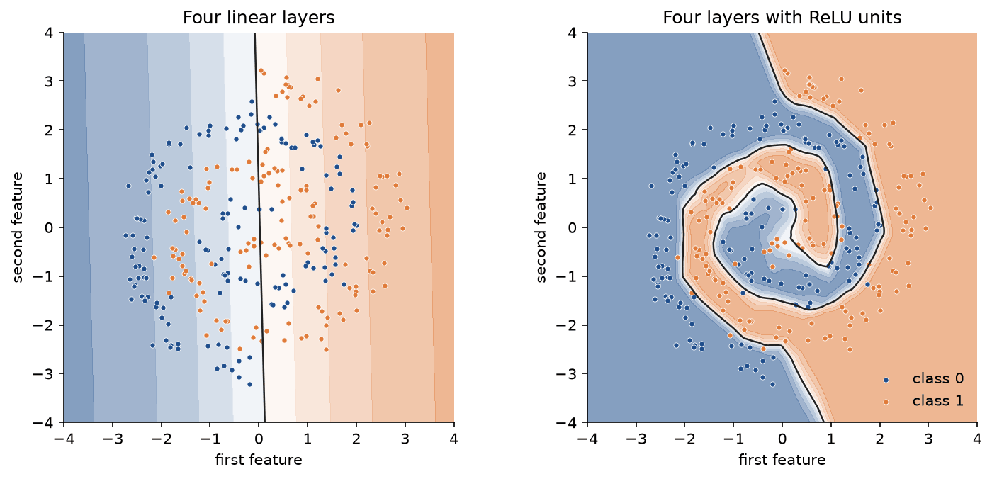
The figure shows a network with three hidden layers of 32 units, trained on two interleaved spirals. Without activations it can only cut the plane in two with a straight line and reaches 64.00 % test accuracy; with ReLU units the same network follows the spirals and reaches 92.33 %. With a non-linear activation the collapse fails, and a single hidden layer with any continuous activation that is not a polynomial can approximate any continuous function on a bounded region arbitrarily well, given enough units. Perceptrons and multilayer networks shows what hidden units compute; this page is about keeping them trainable when there are many layers of them.

Eight activation functions

Three activations are smooth and saturate, softplus on one side only:

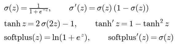
Tanh is a sigmoid stretched to the range from -1 to 1 and centred on zero, with four times the slope at the origin. Softplus is a smooth ReLU, and its derivative is exactly the sigmoid. The other five belong to the rectifier family, which passes positive inputs almost unchanged:

The defaults here are those of PyTorch: α = 0.01 for leaky ReLU and α = 1 for ELU. ReLU has no derivative at exactly z = 0; like PyTorch, the code uses 0 there, and leaky ReLU uses α. GELU keeps its input with probability Φ(z), the chance that a standard normal variable falls below it, which makes it a smooth gate that depends on the input; SiLU, also called swish, gates its input with its own sigmoid. Each derivative follows in a line or two from the chain rule or the product rule:

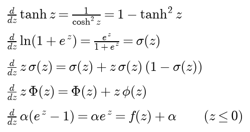
The last line means the ELU backward pass could reuse the stored activation, and with α = 1 the left and right derivatives agree at zero. The sigmoid derivative is derived in Backpropagation. Some pretrained models use a tanh approximation of GELU instead of the exact function:

It differs from the exact GELU by at most 4.73 × 10⁻⁴, at z = -2.699. GELU and SiLU are not monotonic: they dip below zero, GELU to -0.1700 at z = -0.7518 and SiLU to -0.2785 at z = -1.2785, and their slopes slightly exceed one, reaching 1.1289 at z = √2 and 1.0998 at z = 2.3994.

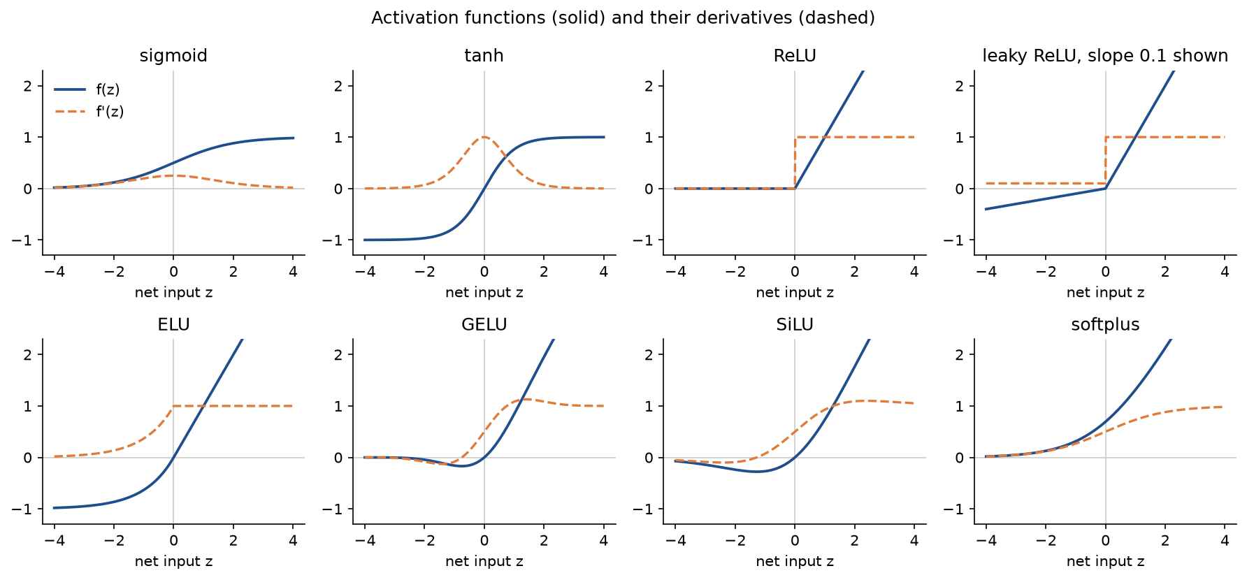
The panels show the shapes the rest of the page reasons about: the sigmoid's slope never exceeds a quarter, tanh's slope is one at the origin and vanishes on both sides, and the rectifiers have slope one for positive inputs and differ in what they do with negative ones. Leaky ReLU is drawn with slope 0.1, because 0.01 would be invisible.

Averages over a Gaussian net input

A net input is a sum of many random terms, so at initialization it is close to Gaussian. The initialization rules below depend on four averages of each activation over a standard normal net input:

The mean measures how far an activation is from zero-centred, E[f(z)²] is what the next layer's variance depends on, E[f'(z)²] is what the backward pass multiplies by, and g is the gain used under A gain for any activation. Computed by numerical integration:

• Sigmoid: mean 0.5000, E[f²] 0.2934, E[f'²] 0.0448, gain 1.8462.
• Tanh: mean exactly 0, E[f²] 0.3943, E[f'²] 0.4644, gain 1.5925.
• ReLU: mean 0.3989, which is one over the square root of 2π, E[f²] and E[f'²] exactly 0.5000, gain √2 = 1.4142.
• Leaky ReLU: mean 0.3950, E[f²] and E[f'²] exactly (1 + α²) / 2 = 0.50005, shown with five decimals because four would hide the slope, gain 1.4141.
• ELU: mean 0.1605, E[f²] 0.6449, E[f'²] 0.6681, gain 1.2452.
• GELU: mean 0.2821, E[f²] 0.4252, E[f'²] 0.4559, gain 1.5335.
• SiLU: mean 0.2066, E[f²] 0.3558, E[f'²] 0.3795, gain 1.6765.
• Softplus: mean 0.8061, E[f²] 0.9212, E[f'²] 0.2934, gain 1.0419.

Saturation and zero-centred outputs

A unit saturates when its net input lies where the activation is flat. The sigmoid's slope is at most 1/4, at z = 0, and drops below 0.01 once the net input is more than about 4.59 away from zero; tanh's slope is 1 at the origin and drops below 0.01 beyond about 2.99. A saturated unit hurts twice. Through B2 it multiplies the error passing back through it by almost zero, and through B4 its own incoming weights receive almost no gradient. ReLU and its relatives do not saturate for positive inputs; ELU saturates for large negative inputs, at -α, which makes its negative outputs robust to noise at the price of a vanishing slope there.

The mean of an activation matters through B4:

If every incoming activation is positive, as with sigmoid and softplus units and with ReLU units wherever they are active, all weights entering unit j get gradients of the same sign, the sign of its error. A single example can then only push all of them up or all of them down together, and reaching a weight vector with mixed signs takes a zig-zag path. Averaging over a mini-batch helps only as far as the error changes sign between examples. The second formula shows the other cost: a non-zero mean activation gives every unit of the next layer an offset that carries no information. Tanh fixes the sigmoid's mean, which is why it trains better in hidden layers, and the same argument is the reason for standardizing the inputs.

Vanishing and exploding gradients

Write the entry-by-entry product in B2 as a diagonal matrix of slopes. The matrix in front of the error of layer l + 1 is then the transposed Jacobian of one layer, because differentiating the net inputs of layer l + 1 with respect to those of layer l gives the weights times the slopes:

Because D is diagonal, it is its own transpose. Unrolling B2 from the output down to layer l:

The error reaching layer l is the output error multiplied by one Jacobian per layer above it. The norm of a product is at most the product of the norms, a transpose has the same spectral norm, and the spectral norm of a diagonal matrix is its largest entry in absolute value, so

For sigmoid units every slope factor is at most 1/4, so if every weight matrix has spectral norm below 4, the bound shrinks geometrically, by the ratio of that norm to 4 per layer. That condition matters. The bound is an upper limit; with weights larger than four an individual factor w σ'(z) can exceed one, but only for net inputs in a narrow band, because large weights also push units into saturation. For ReLU units the slopes are 0 or 1, so the product is a product of weight matrices restricted to the active units, and nothing but the weights decides whether it shrinks or grows.

The bound is pessimistic. The typical behaviour follows from averaging over random weights. Assume the weights of layer l + 1 are independent of its error and of the net inputs of layer l, which is accurate for wide layers. B2 for one unit is then a sum of n_out uncorrelated terms with mean zero, so

The first three factors are the backward factor of one layer. If it is below one at every layer, the error vanishes geometrically towards the input; above one, it explodes. For a sigmoid network with square layers and n v = 1 the factor is E[σ'(z)²], at most 1/16, so the error shrinks at least fourfold per layer in size. No weight scale rescues it: a factor of one would need n v of at least 16, and weights that large saturate the units in the forward pass.

The weight gradient combines both directions. For one example it is the outer product of the error with the activations below, whose norm is the product of the two norms. In a ReLU network whose initial weights all have c times He's standard deviation this has a surprising consequence:

The gradients do not vanish towards the input; they are all wrong by the same factor, exponential in the depth, relative to the weights they update. The measurements below and the sample project both show it.

Dead ReLUs

Call a unit dead on a data set if its net input is at most zero for every example in it. Its activation and its slope are then zero for every example, so B2 gives it zero error, B3 and B4 give its bias and incoming weights zero gradients, and B4 also gives its outgoing weights zero gradients because its activation is zero. In the first hidden layer the unit's inputs are the data, which never change, so it can never recover. Deeper in the network a dead unit can come back if the layers below it move its inputs. Units die when a large update pushes a bias or a weight vector far enough that the net input is negative everywhere, typically because the learning rate is too large. Deep, narrow networks on low-dimensional data also start with some dead units, because each layer maps the data onto a thin set that a unit's half-space can miss entirely.

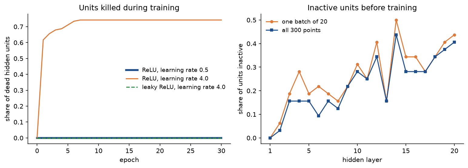
The left panel trains one hidden layer of 128 ReLU units on the spirals. With learning rate 4.0 the network loses 62 % of its units in the first epoch and 74 % after 30, against none at 0.5; leaky ReLU at 4.0 loses none and reaches a lower cost, 0.3638 against 0.4493. The right panel counts the units of a 20-layer, 32-unit He-initialized ReLU network that are inactive before any training: 22.7 % of all hidden units are dead on the 300 training points. Detection needs the whole data set or a large sample, because a unit silent on one mini-batch may fire on the next: in the last layer one batch of 20 suggests 44 % where the full set shows 41 %. The remedies are a smaller learning rate, He initialization with zero biases, normalization layers, or an activation with a non-zero slope for negative inputs. Leaky ReLU keeps a slope of α everywhere, and ELU, GELU and SiLU have slopes that are small but not zero for moderately negative inputs, so none of them has the exact zero that makes the death of a ReLU unit permanent.

Why the weights must not start equal

Suppose every weight entering layer l has the same value and every bias of the layer is the same. Then every unit of the layer has the same net input and the same activation. If, in addition, the weights leaving the layer are equal, B2 gives every unit the same error, because every factor in its sum is the same for all of them, and B4 gives every row of the weight gradient the same values. After the update the rows are still equal, and by induction they stay equal for the whole of training: a layer of n units computes what one unit computes. All-zero weights are the extreme case. B2 multiplies by a zero weight matrix, so no error reaches any hidden layer on the first step, and with ReLU units and zero biases every net input is 0, where the slope is 0, so no weight receives any gradient at all. Random initial weights break the symmetry; biases may start at zero.

Variance through one layer

Take layer l at initialization and assume that its weights are independent with mean 0 and variance v, that they are independent of the layer's inputs, which holds because the inputs depend only on earlier layers, and that the inputs are identically distributed with second moment m and the biases are zero. The mean of a net input is then zero, so its variance is its second moment. Expanding the square of the sum gives a double sum, in which every term with two different weights averages to zero:

Note the second moment m, not the variance of the activations: for ReLU or sigmoid units, whose outputs have a positive mean, the two differ. A net input is a sum of many independent terms, so it is approximately Gaussian, and the second moment of the next activations is an average over a Gaussian:

These two lines are a recursion that predicts the signal size in every layer from the widths, the weight variances and the activation alone; together with the backward factor of the previous sections it predicts the error sizes too.

The diagram is the recipe for every rule that follows: pick v so that the forward factor from one second moment to the next, and the backward factor on the error, are both one.

He initialization for ReLU

For a net input symmetric about zero, ReLU keeps the positive half and zeroes the negative half, so its second moment is half the variance of the net input, and the recursion becomes a single product:

The variance stays constant from layer to layer exactly when one half of n_in times v is one:

The uniform bound follows from the variance of a uniform distribution:

This is He, or Kaiming, initialization. The backward factor for ReLU is n_out times v times one half, since the slope is 1 on half the inputs, so keeping the error variance instead gives v = 2 / n_out, the mode="fan_out" of PyTorch. For square layers the two agree. With a standard deviation c times He's, the variance changes by a factor c² per layer.

Xavier initialization for tanh

Near the origin tanh z is close to z and its slope close to 1, so the second moment of the activations is close to the variance of the net inputs, and the mean squared slope close to 1. The forward and the backward recursion then each ask for their own weight variance:

Both hold only when the layer is square. Glorot and Bengio's compromise is the harmonic mean:

This is Xavier, or Glorot, initialization. For ReLU it is too small by a factor of two in variance per square layer, because it ignores the half that ReLU discards. For tanh it is slightly too small too, because E[tanh(z)²] is smaller than the variance of z away from the origin: the signal shrinks slowly with depth, and PyTorch's calculate_gain("tanh") returns 5/3 to compensate.

A gain for any activation

Writing the weight variance as a gain squared over the fan-in separates the fan-in from a constant that depends only on the activation. For unit-variance net inputs the recursion gives the next variance as the gain squared times E[f(z)²], so the gain that makes unit variance a fixed point is

These are the gains in the list of Gaussian averages. For ReLU the gain is √2, He's constant; for leaky ReLU it is PyTorch's value; for tanh it is 1.5925, close to PyTorch's 5/3; for SiLU and GELU it is 1.6765 and 1.5335. Near the origin SiLU and GELU behave like z/2, so He's √2 halves small signals in every layer; in practice these activations are used with normalization layers, which make the question moot.

No gain helps a deep sigmoid network. Its forward signal never collapses, because E[σ(z)²] is at least 1/4 even for tiny net inputs, but the part that survives is the constant mean 1/2, which carries no information, and the backward factor stays below one for any weight scale that does not saturate the units.

Checking the predictions

The recursions describe an average over random networks. A single network of finite width wanders around it, the more so the narrower and deeper it is; correlations between units, non-zero biases and non-Gaussian inputs in the first layer are ignored, and the backward half rests on the independence assumption above. Within those limits the predictions are close, as a network with 20 hidden layers of 128 units, evaluated at initialization on 500 standard normal inputs with random targets, shows.

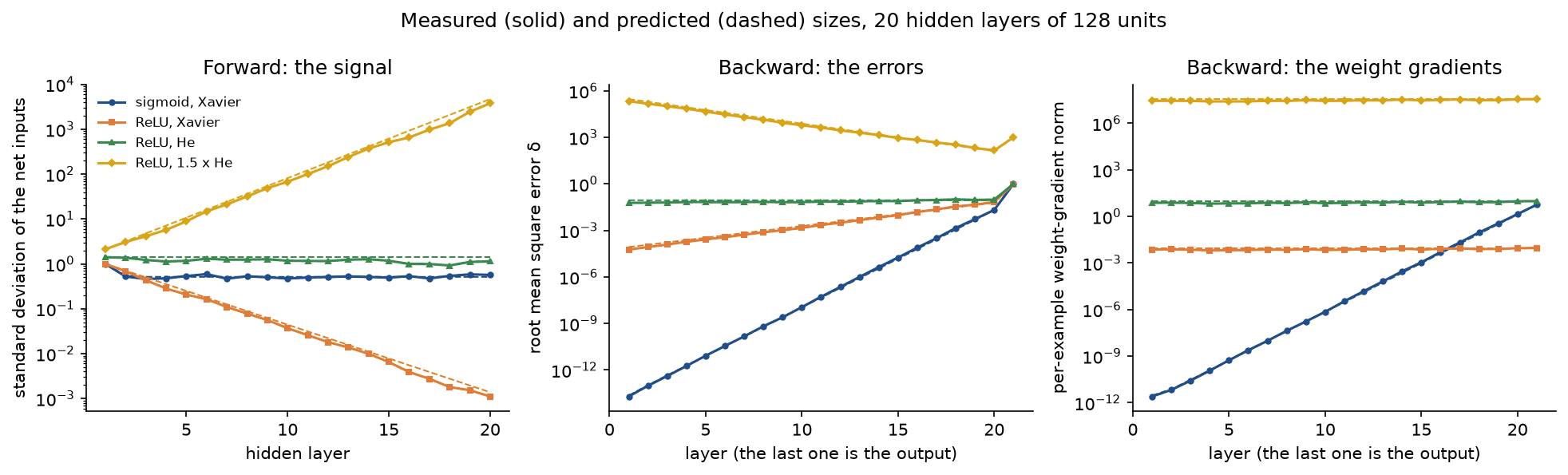
The dashed predictions follow the measured curves closely, and each setting shows one mechanism in isolation:

• Sigmoid with Xavier: the forward signal is healthy, with a standard deviation of about one half in every layer after the first, but the error shrinks from 2.1 × 10⁻² in layer 20 to 2.0 × 10⁻¹⁴ in layer 1, a factor of about 4.3 per layer, and the first layer's weight gradient is 1.8 × 10⁻¹² of the last hidden layer's. This is the vanishing gradient in its pure form.
• ReLU with He: forward and backward sizes stay within a factor of two across all 20 layers, as derived.
• ReLU with Xavier: the forward signal halves in variance per layer, down to a standard deviation of 1.1 × 10⁻³ in layer 20, and the error shrinks by about 1/√2 per layer on the way back. The per-example weight gradients are nevertheless flat across layers, as derived above: between 6.4 × 10⁻³ and 9.2 × 10⁻³ in every layer, against 6.7 to 9.7 for He, about 2⁻¹⁰ times smaller.
• ReLU with 1.5 times He: the signal grows by 1.5 per layer to a standard deviation of 3.8 × 10³ in layer 20, the error grows by about 1.5 per layer on the way back, and the weight gradients lie between 2.6 × 10⁷ and 3.6 × 10⁷ in every layer.

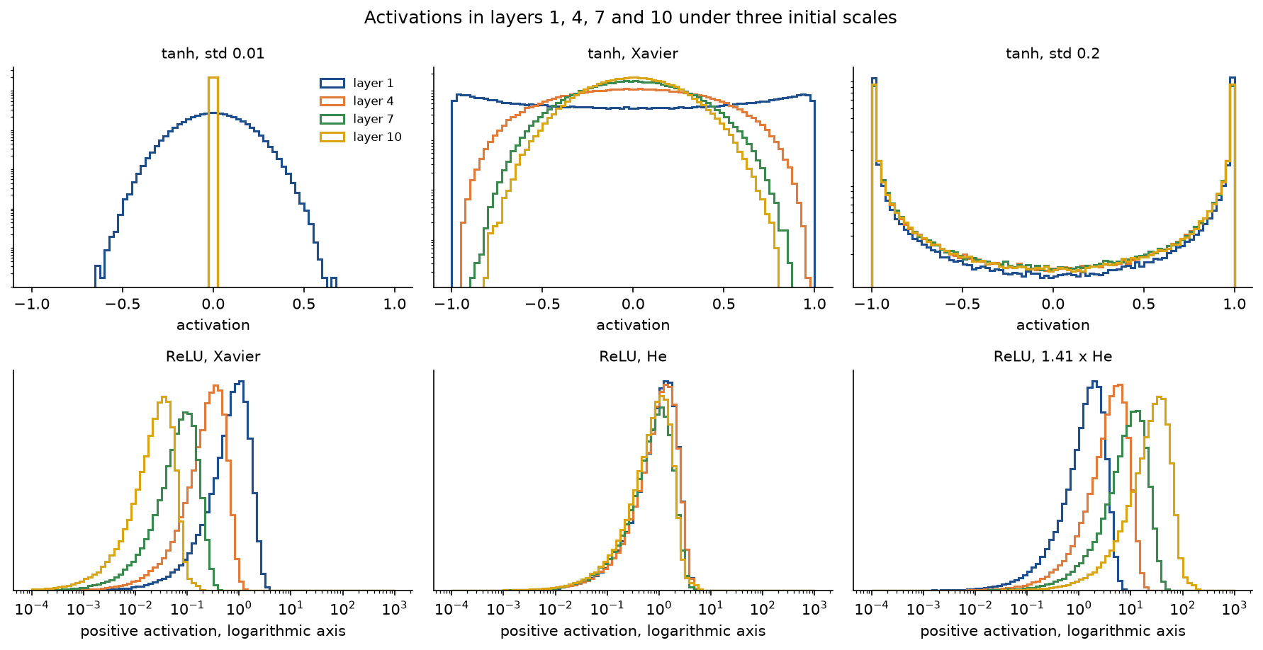
Activation histograms make the same point for the forward pass, in ten layers of 256 units. With tanh units and weights of standard deviation 0.01 the activations collapse to zero, with a standard deviation of 0.156 in layer 1 and below 10⁻⁴ from layer 6 on; with 0.2 they pile up at the limits, 33.4 % of them beyond 0.99 in magnitude in layer 10; Xavier keeps a spread distribution that narrows slowly, to a standard deviation of 0.2308 by layer 10. With ReLU units, Xavier shrinks the standard deviation of the activations from 0.5829 to 0.0215 over ten layers, He keeps it between 0.64 and 0.86, and √2 times He inflates it from 1.1658 to 21.9995. In the same tanh network the standard deviation of the net inputs of layer 10 is 0.2440 under Xavier against a predicted 0.2409; the gain 5/3 holds it at 1.1063 (predicted 1.0858) with 1.66 % of the units saturated, and the fixed-point gain 1.5925 at 1.0199 (predicted 1.0003) with 0.94 %. Orthogonal initialization, which draws a weight matrix with orthonormal rows scaled by the gain, keeps every singular value of a linear layer at the gain and is popular for recurrent networks.

Normalization and residual connections

Initialization fixes the scale once; two architectural devices keep it fixed during training as well, and together with good initialization they are what makes networks of hundreds of layers trainable. Batch normalization replaces each net input by its standardized value over the mini-batch, with a small constant ε for safety, followed by a learned scale and shift:

Layer normalization does the same with the mean and variance over the units of one example. Either way the layer's output no longer depends on the scale of its weights, since multiplying the weights by a positive c multiplies the net inputs and their standard deviation by c, so a bad initial scale cannot compound from layer to layer, and the backward pass divides by the same standard deviation. A residual connection adds a layer's input to its output:

The gradient with respect to the activations passes through each block unchanged plus a correction, so the product of Jacobians always contains the identity path. The forward variance, on the other hand, adds up over the blocks unless the branches are scaled down, which is why residual networks are combined with normalization or with branches initialized near zero.

In a network with 20 hidden layers of 64 units, a tanh network with weights of standard deviation 0.01 has a first-layer weight-gradient norm of 4.1 × 10⁻²³ as a plain stack, 2.08 with batch normalization, 1.75 with layer normalization and 4.3 × 10⁻² with residual blocks. For a ReLU network at twice He's standard deviation the plain stack's gradient norms are 1.9 × 10¹¹ in the first layer and 1.2 × 10¹² in the last hidden one; batch and layer normalization bring them to between 0.49 and 26.5, while residual blocks alone make them larger still, 9.5 × 10¹⁵ and 2.2 × 10¹⁷. Training image classifiers uses batch normalization, The transformer architecture uses layer normalization with residual connections, and Recurrent networks meets the same products of Jacobians through time.

Worked example

Four small calculations that can be done with a pen. Values are computed in double precision and shown to four decimals; where a hand calculation from rounded terms differs in the last digit, that is pointed out. Every number is asserted by tests/test_worked_example.py and tests/test_linear_collapse.py and printed by examples/worked_example.py.

Two linear layers are one

Two inputs, three hidden units with the identity as activation, one output. The hidden weights W1 have rows (1.0, -2.0), (0.5, 1.0) and (-1.5, 0.5), the hidden biases b1 are (0.5, -1.0, 0.0), the output weights W2 form the row (2.0, -1.0, 1.0) and the output bias b2 is 0.5. The collapsed layer has

• weight W2 W1 = (2.0 - 0.5 - 1.5, -4.0 - 1.0 + 0.5) = (0, -4.5),
• bias W2 b1 + b2 = 1.0 + 1.0 + 0.0 + 0.5 = 2.5.

For the input x = (1, 2) the two-layer network computes the hidden net inputs (1 - 4 + 0.5, 0.5 + 2 - 1, -1.5 + 1 + 0) = (-2.5, 1.5, -0.5) and then the output 2 × (-2.5) - 1.5 + (-0.5) + 0.5 = -6.5; the collapsed layer computes 0 × 1 - 4.5 × 2 + 2.5 = -6.5. The same. With a ReLU between the layers the hidden activations become (0, 1.5, 0) and the output -1.5 + 0.5 = -1.0: two of the three hidden units are switched off for this input, and no single matrix can reproduce a computation in which the set of active units depends on the input.

The eight activations at three points

Each activation evaluated at z = -1.5, 0 and 0.5, then its derivative at the same three points:

• Sigmoid: values 0.1824, 0.5000, 0.6225; slopes 0.1491, 0.2500, 0.2350.
• Tanh: values -0.9051, 0, 0.4621; slopes 0.1807, 1, 0.7864.
• ReLU: values 0, 0, 0.5000; slopes 0, 0, 1.
• Leaky ReLU: values -0.0150, 0, 0.5000; slopes 0.0100, 0.0100, 1.
• ELU: values -0.7769, 0, 0.5000; slopes 0.2231, 1, 1.
• GELU: values -0.1002, 0, 0.3457; slopes -0.1275, 0.5000, 0.8675.
• SiLU: values -0.2736, 0, 0.3112; slopes -0.0413, 0.5000, 0.7400.
• Softplus: values 0.2014, 0.6931, 0.9741; slopes 0.1824, 0.5000, 0.6225.

Each entry follows from the formulas with e to the 1.5 = 4.4817, e to the -0.5 = 0.6065, Φ(-1.5) = 0.0668, φ(1.5) = 0.1295, Φ(0.5) = 0.6915 and φ(0.5) = 0.3521. For example σ(-1.5) = 1 / (1 + 4.4817) = 0.1824, and the GELU slope at -1.5 is 0.0668 - 1.5 × 0.1295 = -0.1275 at full precision (the rounded terms give -0.12745), negative because GELU decreases there. The softplus slope at -1.5 equals σ(-1.5). At z = -1.5 the rectifiers differ the most: ReLU passes no gradient, leaky ReLU passes one hundredth, and ELU passes e to the -1.5 = 0.2231.

The error through a chain of four units

One unit per layer, four layers, with weights w1 to w4 equal to 0.8, 1.5, 1.2 and 2.0 and biases b1 to b4 equal to 0.2, -0.5, 0.1 and -1.0, the same activation in the three hidden layers, an identity output, input x = 1, target y = 1 and the squared-error cost. With one unit per layer the backpropagation equations become products of numbers:

With sigmoid hidden units, layer by layer from the input:

• Layer 1: net input 1.0000, activation 0.7311, slope 0.1966, error -0.0198, weight gradient -0.0198.
• Layer 2: net input 0.5966, activation 0.6449, slope 0.2290, error -0.0672, weight gradient -0.0492.
• Layer 3: net input 0.8739, activation 0.7055, slope 0.2078, error -0.2447, weight gradient -0.1578.
• Layer 4, the output: net input and output 0.4111, error 0.4111 - 1 = -0.5889, weight gradient -0.4155.

The forward pass starts with 1.5 × 0.7311 - 0.5 = 0.5966 at full precision (0.59665 from the rounded terms), and the cost is one half of (0.4111 - 1) squared, 0.1734. Going back, each step multiplies the error by the next weight times the sigmoid slope: by 2.0 × 0.2078 = 0.4155 into layer 3 (0.4156 from the rounded slope), by 1.2 × 0.2290 = 0.2748 into layer 2 and by 1.5 × 0.1966 = 0.2949 into layer 1. The first layer's error is 0.0337 of the output error, about a thirtieth after three steps, although every weight the error passes through is larger than one.

With ReLU hidden units and the same weights and biases every unit is active, so the slopes are all one and only the weights remain:

• Net inputs 1.0, 1.0, 1.3 and 1.6, equal to the activations.
• Errors 2.16, 1.44, 1.2 and 0.6 from layer 1 to the output: 2.0 × 0.6 = 1.2, then 1.2 × 1.2 = 1.44, then 1.5 × 1.44 = 2.16.
• Weight gradients 2.16, 1.44, 1.2 and 0.78, and the cost one half of 0.6 squared, 0.18.

The error grows by 2.0 × 1.2 × 1.5 = 3.6 on its way back: ReLU has removed the slope factor, and what is left is decided by the weights, which is the job of initialization.

Had the second bias been -2.0 instead of -0.5, the second net input would be 1.5 - 2.0 = -0.5 and the second ReLU unit off. The output becomes 2.0 × 0.1 - 1.0 = -0.8 with cost 1.62, the errors of layers 4 and 3 are -1.8 and -3.6, but the error of layer 2 is 1.2 × 0 × (-3.6) = 0, the error of layer 1 is 0 as well, and the third weight's gradient is the error of layer 3 times the zero activation of layer 2, 0 too. Five of the eight parameters receive no gradient: an inactive unit cuts the chain in both directions.

Initial scales of one layer

For a layer with 300 inputs and 100 outputs:

• Xavier: weight variance 2 / (300 + 100) = 0.005, normal standard deviation 0.0707, uniform bound the square root of 6 / 400, 0.1225.
• He: weight variance 2 / 300 = 0.0067, standard deviation 0.0816, uniform bound the square root of 6 / 300, 0.1414.
• The default of torch.nn.Linear: weight variance 1 / (3 × 300) = 1 / 900, standard deviation 1 / 30 = 0.0333, uniform bound one over the square root of 300, 0.0577.

For inputs of second moment 1 the net inputs have variance 300 times the weight variance: 1.5 for Xavier, 2 for He and 1/3 for the default. After a ReLU the second moments are half of that, 0.75, 1 and 1/6, so only He hands the next layer inputs of the same second moment it received. In a stack of square ReLU layers the per-layer variance factor, one half of n times v, is therefore 1 for He, 1/2 for Xavier and 1/6 for the default. After ten layers that is 1, 2⁻¹⁰ = 0.0010 and 6⁻¹⁰ = 1.65 × 10⁻⁸ in variance, or 1, 1/32 = 0.03125 and 1.28 × 10⁻⁴ in standard deviation.

The code

The package activations_and_initialization is plain NumPy, split into one module per idea. PyTorch is imported only inside the functions of comparisons.py and architectures.py, so everything else works without it.

• arrays.py holds the Array type, as_array and as_matrix, which insists on one example per row.
• gaussian.py holds the normal density and distribution function and gaussian_expectation, which averages any function over a Gaussian net input by quadrature.
• activations.py holds the eight activations, the tanh form of GELU and the identity, each with its derivative, collected in ACTIVATIONS; CATALOGUE lists the eight in the order of this page.
• linear_collapse.py multiplies out a stack of affine layers.
• losses.py, propagation.py and network.py are the forward and backward passes of Backpropagation in mini-batch form and the frozen Network class, with cross-entropy computed from the output net input so that it stays finite when the sigmoid saturates.
• gradient_check.py compares the backward pass with central differences for every activation.
• initialization.py holds the fan-in and fan-out of the (outputs, inputs) layout, recommended_gain, the Xavier, He and torch.nn.Linear scales, initialize_weights, initialize_network and constant_network.
• variance.py holds the Gaussian averages of each activation, the fixed-point gain and predict_variances, the forward and backward recursions.
• measurements.py holds per-layer statistics, batch and per-example weight-gradient norms, error sizes, dead-unit masks and the saturated share.
• datasets.py generates the two spirals and standard normal probe batches from a seed.
• training.py runs mini-batch gradient descent, recording a run that overflows as nan instead of raising.
• worked_example.py builds and prints the four calculations above.
• signal_profile.py measures and predicts the sizes per layer of a deep network at initialization, with the settings compared on this page.
• study.py holds the ten configurations of the sample project, trains them and classifies each run.
• pitfalls.py holds the demonstrations behind the Pitfalls section.
• comparisons.py and architectures.py hold the same activations, initializers, gradients and training runs in PyTorch, and the normalized and residual stacks.
• plotting.py and depth_plots.py draw every figure in the handbook's four colours and save it reproducibly.

Python counts from zero, so weights[0] is W1 and deltas[0] is Δ1, as in Backpropagation; ForwardPass.activations[l] is the activation of layer l because it starts with the inputs. The forward recursion in variance.py is a few lines:

second_moment = input_second_moment
for fan_in, variance, name in zip(layer_sizes[:-1], weight_variances, activations):
    q = fan_in * variance * second_moment
    function = ACTIVATIONS[name].function
    second_moment = gaussian_expectation(lambda z: function(z) ** 2, q)

gaussian_expectation folds the integral onto the positive half line and applies 200-point Gauss-Legendre quadrature on the interval from 0 to 12, beyond which the normal density is below 10⁻³¹:

Every activation here is smooth on each side of zero, so the folded integrand is smooth even for ReLU, whose kink sits on the fold, and the result is accurate to rounding: the ReLU mean comes out as one over the square root of 2π to 13 digits. GELU needs the error function, which NumPy lacks; erf applies the standard library's math.erf entry by entry, accurate to rounding but slow, which is why the sample project leaves GELU out.

The examples and the project import the package, so install the repository first as described in the main README. The examples each demonstrate one idea and run in under ten seconds from the repository root:

• examples/worked_example.py prints every value of the worked example.
• examples/activation_gallery.py draws the activations and their derivatives, prints where GELU and SiLU dip and peak, and prints the Gaussian averages next to PyTorch's recommended gains.
• examples/signal_propagation.py measures and predicts the sizes per layer of a 20-layer network, draws the activation histograms, checks the tanh gains and measures normalized and residual stacks in PyTorch.
• examples/dead_units.py kills ReLU units with a large learning rate and counts the units a fresh deep network has lost.
• examples/common_mistakes.py demonstrates the missing activation, the constant start, PyTorch's default scale, the wrong fan-in axis, the uniform bound used as a standard deviation and the gain computed from the variance.
• examples/compare_with_pytorch.py checks activations, gains, initializers, gradients and a whole training run against PyTorch.

python neural-networks/activations-and-initialization/examples/worked_example.py
python neural-networks/activations-and-initialization/examples/activation_gallery.py
python neural-networks/activations-and-initialization/examples/signal_propagation.py
python neural-networks/activations-and-initialization/examples/dead_units.py
python neural-networks/activations-and-initialization/examples/common_mistakes.py
python neural-networks/activations-and-initialization/examples/compare_with_pytorch.py

The sample project, project/initialization_study.py, puts the theory to a realistic test. It trains one network, 20 hidden layers of 32 units with a sigmoid output and the cross-entropy cost, on 300 points of two noisy interleaved spirals by plain mini-batch gradient descent with learning rate 0.01, batches of 20 and 150 epochs, under ten choices of hidden activation and initial scale, from three seeds each, and measures test accuracy on 300 fresh points. Before training it checks the gradients of a small version of the network and records the weight-gradient norm of every layer on the whole training set. Every run is then classified by its late cost, the median training cost over its last 15 epochs: a run trains if the late cost is below half of ln 2, the cost of a network that outputs one half everywhere; it stalls at chance within 0.01 of ln 2; it diverges if the cost overflows; and anything between learns slowly. A configuration takes the verdict of the median late cost over its seeds. The late cost rather than the last epoch decides, because plain gradient descent on a deep network without normalization runs close to the edge of stability, and a single epoch can spike. "ReLU, Linear default" draws weights with the variance of PyTorch's default, a third of 1 / n_in; "1.41 x He" uses √2 times He's standard deviation; "SiLU, gain 1.68" uses SiLU's fixed-point gain instead of He's √2. Options such as --configurations, --seeds, --depth, --width, --epochs and --learning-rate change the setup, and --figures sends the two PNGs elsewhere so a custom run does not overwrite the ones shown here; the default run takes under a minute.

python neural-networks/activations-and-initialization/project/initialization_study.py
python neural-networks/activations-and-initialization/project/initialization_study.py --configurations relu-he,relu-xavier --depth 40

With the defaults the ten configurations end as follows, with the late cost of each seed and the test accuracy averaged over the seeds:

• ReLU, Linear default: late costs 0.6931 in all three seeds, test accuracy 0.5000; stalls at chance.
• ReLU, Xavier: 0.6313, 0.6931 and 0.5812, test accuracy 0.5989; learns slowly, and one seed never leaves chance.
• ReLU, He: 0.3439, 0.1978 and 0.1237, test accuracy 0.8956; trains.
• ReLU, 1.41 x He: the initial cost is 523.9 and every seed overflows in the first epoch; diverges.
• Sigmoid, Xavier: 0.6932, 0.6932 and 0.6931, test accuracy 0.5000; stalls at chance.
• Tanh, Xavier: 0.6026, 0.4312 and 0.3785, test accuracy 0.6922; learns slowly.
• Tanh, Xavier with gain 5/3: 0.3068, 0.0424 and 0.0836, test accuracy 0.8344; trains.
• ELU, He: 0.0636, 0.0382 and 0.0560, test accuracy 0.9311; trains, the fastest and most consistently.
• SiLU, He: 0.6922, 0.3559 and 0.3263, test accuracy 0.6600; learns slowly, and one seed stays at chance.
• SiLU, gain 1.68: 0.1215, 0.0331 and 0.0330, test accuracy 0.9344; trains.

Every prediction of the theory shows up. The sigmoid network and the ReLU network at PyTorch's default scale never leave chance; ReLU with Xavier barely moves; at √2 times He the first steps overflow. He initialization trains. Among the saturating activations, tanh with plain Xavier learns slowly, while the gain of 5/3, which holds the signal near its fixed point, makes it train. Among the rectifiers, SiLU with He is under-scaled for the reason given under A gain for any activation, while SiLU with its own fixed-point gain comes close to ELU. The test accuracy belongs to the network after the last epoch, so a late spike can lower it, which is why tanh with gain 5/3 tests lower than its late costs suggest.

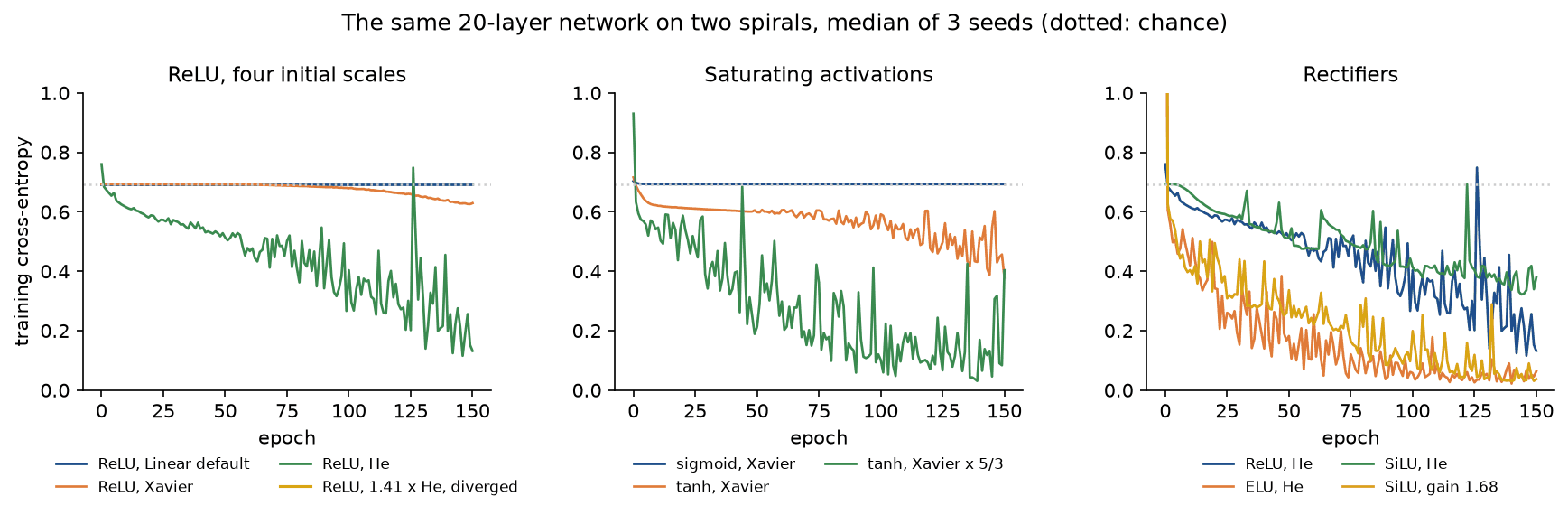
The curves are jagged: plain gradient descent on a 20-layer network without normalization runs close to the edge of stability, and single epochs spike. Normalization layers, momentum and learning-rate schedules smooth this out; Optimizers covers the last two. The spikes also make the run sensitive to rounding, so the individual numbers above can come out differently on another computer, as In practice shows, while which configurations train and which stay at chance does not change.

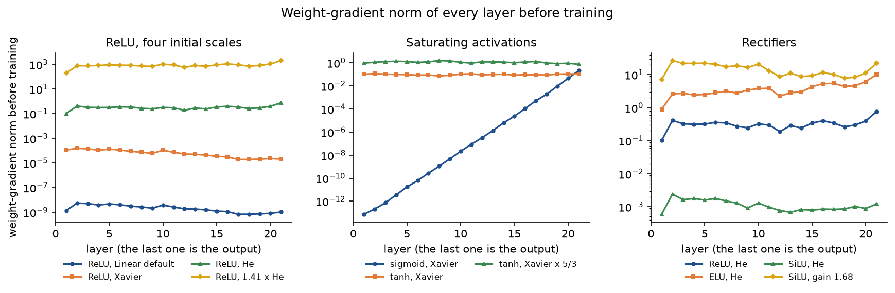
The gradient norms before training already tell the outcome. The sigmoid network's first-layer gradient is 7.35 × 10⁻¹⁴, 1.6 × 10⁻¹² of its last hidden layer's: the vanishing gradient. The four ReLU scales give flat lines, the c to the L - 1 rule derived above: Xavier's first-layer norm, 1.11 × 10⁻⁴, is about a thousandth of He's 0.102, close to 2⁻¹⁰; the default's, 1.36 × 10⁻⁹, is 1.3 × 10⁻⁸ of He's, close to 6⁻¹⁰ = 1.65 × 10⁻⁸; and that of 1.41 times He, 196, is about 1,900 times He's, the order of 2¹⁰. The rule is only approximate at the output, because the sigmoid output and cross-entropy pass back an error that does not scale with the weights. SiLU with He starts four orders of magnitude below SiLU with its fixed-point gain, which is why it learns slowly.

The notebook activations_and_initialization.ipynb is a guided tour in the order of this page: the collapse of linear layers, the activations and their averages, the chain, the depth profiles, symmetric and constant starts, the variance of one layer, histograms, dead units, normalization, a short version of the study and the comparisons with PyTorch. The tests in tests check the worked example value by value, the Gaussian averages, the recursions against wide random networks, the gradients against finite differences and against PyTorch, and the study's classification, and run in a few seconds:

python -m pytest neural-networks/activations-and-initialization

The two spirals and the probe batches are synthetic, generated from a seed, so nothing is downloaded and no licence is involved.

In practice

The PyTorch idiom for the initializations of this page:

import torch

hidden = torch.nn.Linear(300, 100)
torch.nn.init.kaiming_normal_(hidden.weight, mode="fan_in", nonlinearity="relu")
torch.nn.init.zeros_(hidden.bias)
bounded = torch.nn.Linear(100, 100)
torch.nn.init.xavier_uniform_(bounded.weight, gain=torch.nn.init.calculate_gain("tanh"))
torch.nn.init.zeros_(bounded.bias)
model = torch.nn.Sequential(
    hidden, torch.nn.ReLU(), bounded, torch.nn.Tanh(), torch.nn.Linear(100, 1)
)

Our implementation agrees with PyTorch everywhere the two can be compared, as examples/compare_with_pytorch.py and tests/test_comparisons.py check:

• Values and derivatives of the eight activations and of the tanh form of GELU agree with torch.nn and autograd to within 5 × 10⁻¹⁵ on 1,001 points between -25 and 25, except softplus: torch.nn.Softplus returns z itself for z above 20, a deliberate shortcut that differs from the exact value by about e to the -20, 2.0 × 10⁻⁹.
• recommended_gain equals torch.nn.init.calculate_gain for every nonlinearity it supports, and our initializers and torch.nn.init.xavier_normal_, xavier_uniform_, kaiming_normal_ and kaiming_uniform_ produce weights with the same standard deviation, 0.0500 or 0.0632 for a 300 by 500 matrix within sampling error, and uniform weights reaching the same bound. The random numbers themselves differ, because the generators do.
• Our backward pass and autograd agree to 8.9 × 10⁻¹⁶ on small networks for every activation, and to 9.0 × 10⁻¹⁷ on one batch of the project's He-initialized ReLU network.
• The project's He-initialized ReLU run repeated with torch.optim.SGD from the same weights and batches follows our loss curve to within 1.5 × 10⁻¹³ for the first 100 epochs. At epoch 125 the difference passes 10⁻⁶ and the runs separate, ending at costs of 0.3439 and 0.3085.

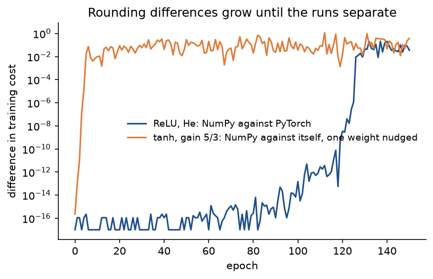
That separation is the training dynamics, not a disagreement: changing one first-layer weight of the tanh network with gain 5/3 by one unit in the last place, 6.9 × 10⁻¹⁸, separates our run from itself after 4 epochs. Compare implementations by their gradients, which agree to rounding, not by the end of a long unstable run.

To diagnose a network that will not train, record per layer the norm of the weight gradient (parameter.grad.norm() in PyTorch), the spread of the activations and the share of dead units on a large sample, before training and every few epochs, and read them as the diagram shows. In every one of these cases batch or layer normalization also helps, because it keeps a bad scale from compounding across layers. Against exploding gradients that remain, torch.nn.utils.clip_grad_norm_ rescales the whole gradient when its norm exceeds a threshold.

When to use which:

• ReLU with He initialization (kaiming_normal_ or kaiming_uniform_ with nonlinearity="relu") is the default for fully connected and convolutional networks without normalization. Leaky ReLU and ELU are drop-in replacements when dead units are a problem.
• GELU is the standard activation of transformer blocks and SiLU of many convolutional networks and of the gated feed-forward layers of recent language models; both come with layer or batch normalization, which removes most of the sensitivity to the initial scale.
• Tanh belongs in recurrent cells and in places that need bounded, zero-centred outputs; initialize it with Xavier and gain 5/3, or orthogonally in recurrent weight matrices.
• Sigmoid belongs in output layers that produce probabilities and in gates that switch something on or off, not in the hidden layers of a deep stack.
• Softplus is the smooth choice where an output must be positive, such as a predicted standard deviation.
• torch.nn.Linear and torch.nn.Conv2d initialize with kaiming_uniform_(a=math.sqrt(5)), a variance of one third of 1 / n_in. That is harmless in shallow networks and in networks with normalization, and too small for a deep plain ReLU stack, where the explicit He initialization above is needed.
• Use the from-scratch code to see where a gradient vanishes and why, and the library for everything else.

Pitfalls

• A missing activation. A stack of Linear layers without activations between them is one linear map, however deep. examples/common_mistakes.py builds three torch.nn.Linear layers and reproduces their outputs with one collapsed matrix, and on two spirals a four-layer linear network reaches 64.00 % test accuracy against 92.33 % with ReLU units.
• Sigmoid in the hidden layers of a deep network. Its slope is at most 1/4, so the error shrinks about fourfold per layer, and no initial scale fixes it. In the sample project the 20-layer sigmoid network stays at chance in all three seeds.
• Believing ReLU alone cures vanishing gradients. ReLU removes the slope factor, not the weight factor. With Xavier initialization or PyTorch's default scale, the 20-layer ReLU network of the sample project hardly trains or does not train at all.
• An initialization matched to the wrong activation. Xavier halves the variance per layer in a ReLU network; He halves small signals in a SiLU or GELU network, whose slope at the origin is 1/2. Match the gain to the activation, as under A gain for any activation; in the sample project SiLU with He learns slowly and SiLU with its fixed-point gain trains.
• Trusting PyTorch's default to be He. torch.nn.Linear draws weights with a sixth of He's variance. After 20 default ReLU layers of 64 units the outputs vary across 1,000 different inputs by 8.67 × 10⁻⁹, against 0.132 with kaiming_normal_ and zero biases: what is left is the biases, the same for every input. examples/common_mistakes.py prints both.
• Reading the fan-in from the wrong axis. In the (outputs, inputs) layout of torch.nn.Linear.weight and of this page the fan-in is shape[1]. Using shape[0] for a layer with 300 inputs and 100 outputs makes the He standard deviation 0.1414 instead of 0.0816, √3 times too large; for square layers the mistake is invisible.
• Confusing the uniform bound with the standard deviation. A uniform distribution on the interval from -r to r has standard deviation r over √3. Using He's uniform bound as a normal standard deviation triples the variance of every layer; after ten ReLU layers of 256 units the measured variance is 59049 = 3¹⁰ times too large, exactly, because scaling every weight of a ReLU stack with zero biases scales its outputs by the same factor per layer.
• Using the variance of the activations instead of their second moment. The recursion needs the mean of the squared activation, and for ReLU the two differ:

The factor (π - 1) / (2π) is 0.3408, which would give a gain of 1.7129 instead of √2, as examples/common_mistakes.py prints.

• Stating the vanishing-gradient argument without its condition. The product of factors w σ'(z), each at most w/4, is guaranteed to shrink only if the weights are smaller than four in magnitude, and an argument that drops the condition also hides the possibility of exploding gradients. The chain of the worked example shows the opposite case for ReLU: with weights above one its error grows by 3.6 in three steps.
• Dead ReLUs from a learning rate that is too large, or counted on too small a sample. In examples/dead_units.py one hidden layer of 128 ReLU units trained with learning rate 4.0 loses 62 % of its units in the first epoch and 74 % after 30, against none at 0.5, while leaky ReLU at 4.0 loses none. Count dead units on the whole training set or a large sample: one batch of 20 overstates them.
• Constant initial weights. Units that start equal stay equal. The four-layer ReLU network started with every weight at 0.2 keeps identical rows in every weight matrix and reaches 61.00 % test accuracy, against 92.33 % from a random He start, as examples/common_mistakes.py shows.
• Mixing the exact and approximate GELU, or two slopes of leaky ReLU. torch.nn.GELU() and torch.nn.GELU(approximate="tanh") differ by up to 4.7 × 10⁻⁴, enough to fail a tight agreement test and to shift a converted model. Leaky ReLU's slope is 0.01 in PyTorch, while some texts write the maximum of 0.1z and z; state the slope whenever the activation is named.
• Expecting two libraries to produce the same training curve. Gradients agree to rounding; a long run on an unstable network does not, because rounding differences grow until the runs separate, at epoch 125 for the project's ReLU network and after 4 epochs for the tanh network nudged by 6.9 × 10⁻¹⁸.

Further reading

• X. Glorot and Y. Bengio, "Understanding the difficulty of training deep feedforward neural networks", AISTATS 2010. Derives the Xavier initialization and measures activations and gradients layer by layer.
• K. He, X. Zhang, S. Ren and J. Sun, "Delving deep into rectifiers: surpassing human-level performance on ImageNet classification", ICCV 2015. The He initialization and the fan-in and fan-out modes.
• Y. LeCun, L. Bottou, G. B. Orr and K.-R. Müller, "Efficient BackProp", in Neural Networks: Tricks of the Trade, Springer, 1998. Zero-centred inputs and activations, and the scale of one over the square root of the fan-in.
• S. Hochreiter, Untersuchungen zu dynamischen neuronalen Netzen, diploma thesis, Technische Universität München, 1991, and Y. Bengio, P. Simard and P. Frasconi, "Learning long-term dependencies with gradient descent is difficult", IEEE Transactions on Neural Networks 5(2), 157-166, 1994. The vanishing gradient problem.
• R. Pascanu, T. Mikolov and Y. Bengio, "On the difficulty of training recurrent neural networks", ICML 2013. Exploding gradients and gradient clipping.
• X. Glorot, A. Bordes and Y. Bengio, "Deep sparse rectifier neural networks", AISTATS 2011. ReLU in deep networks.
• D.-A. Clevert, T. Unterthiner and S. Hochreiter, "Fast and accurate deep network learning by exponential linear units (ELUs)", ICLR 2016.
• D. Hendrycks and K. Gimpel, "Gaussian error linear units (GELUs)", arXiv:1606.08415, 2016.
• S. Elfwing, E. Uchibe and K. Doya, "Sigmoid-weighted linear units for neural network function approximation in reinforcement learning", Neural Networks 107, 3-11, 2018, and P. Ramachandran, B. Zoph and Q. V. Le, "Searching for activation functions", arXiv:1710.05941, 2017. SiLU, also called swish.
• M. Leshno, V. Ya. Lin, A. Pinkus and S. Schocken, "Multilayer feedforward networks with a nonpolynomial activation function can approximate any function", Neural Networks 6(6), 861-867, 1993.
• B. Poole, S. Lahiri, M. Raghu, J. Sohl-Dickstein and S. Ganguli, "Exponential expressivity in deep neural networks through transient chaos", NeurIPS 2016. The variance recursion and its fixed points.
• A. M. Saxe, J. L. McClelland and S. Ganguli, "Exact solutions to the nonlinear dynamics of learning in deep linear neural networks", ICLR 2014. Deep linear networks and orthogonal initialization.
• L. Lu, Y. Shin, Y. Su and G. E. Karniadakis, "Dying ReLU and initialization: theory and numerical examples", Communications in Computational Physics 28(5), 1671-1706, 2020.
• S. Ioffe and C. Szegedy, "Batch normalization: accelerating deep network training by reducing internal covariate shift", ICML 2015; J. L. Ba, J. R. Kiros and G. E. Hinton, "Layer normalization", arXiv:1607.06450, 2016; K. He, X. Zhang, S. Ren and J. Sun, "Deep residual learning for image recognition", CVPR 2016.
• I. Goodfellow, Y. Bengio and A. Courville, Deep Learning, sections 6.3 and 8.4, MIT Press, 2016. Hidden units and parameter initialization.