Anomaly detection

An anomaly detector has to find readings that do not fit, usually without labelled examples of what not fitting looks like, and with anomalies so rare that a detector which flags nothing is already 99 % accurate. Sensor faults, intrusions, fraud and failing machines all reach us this way. This page builds three families of detectors from first principles: statistical baselines (z-scores, the median absolute deviation and rolling-window features), the Isolation Forest, implemented from scratch with its path-length normalizer derived, and a reconstruction-error detector built on a small autoencoder. Each is worked through with small numbers, then run on a simulated pump with five sensors and labelled injected faults, scored with precision, recall, precision-recall curves and detection delays, and checked against scikit-learn and PyTorch. Afterwards you will be able to say which detector suits which kind of anomaly, compute an Isolation Forest score by hand, choose a threshold without fooling yourself, and recognise the settings that make a detector report numbers fixed in advance. It builds on Evaluation metrics for precision and recall, on Decision trees and Ensembles for the forest, and on Backpropagation for the autoencoder.

To run the code in this topic, install the base group, the ml group for the comparisons with scikit-learn, and the deep group for the comparison with PyTorch.

Intuition

An anomaly is a reading that the process generating the data would rarely produce. That definition already shows the two ways to find one. You can model what normal data look like and measure how far a reading is from the model: a z-score measures distance from the mean in standard deviations, and an autoencoder measures how badly a model trained on normal data reconstructs the reading. Or you can skip modelling the normal data and ask how easy a reading is to separate from the rest, which is what an Isolation Forest does.

Anomalies come in three kinds, and no single detector sees all of them:

• A point anomaly is unusual on its own. On the pump below, one reading of one sensor jumps far from its normal range.
• A contextual anomaly is normal in general but unusual in its context. Daytime flow at 02:00 is a perfectly ordinary daytime value, and at night it means a leak.
• A collective anomaly is a sequence of plausible readings that is implausible as a whole: a sensor repeating the same value for six hours, a slow drift, or the motor current rising while the flow stays put.

A detector produces a score per reading, and a separate decision turns scores into flags: a threshold. The two are evaluated separately. The ranking that the score induces is judged by the precision-recall curve and its average precision, and the threshold by the precision, recall and F1 of the flags it produces. Many of the mistakes collected under Pitfalls come from mixing the two, for example a threshold rule that fixes the number of flags before looking at the data.

The Isolation Forest rests on one observation: anomalies are few and different, so random cuts separate them from everything else quickly. Pick a random feature, cut at a random value between its smallest and largest value, repeat on each side, and a point far from the rest ends up alone after a few cuts while a point in a dense region needs many. The number of cuts needed, averaged over many random trees, is the anomaly signal. The worked example traces one such tree by hand.

Spikes and drift show why detectors differ. A spike is a single reading far from its neighbours: any detector that compares a reading with its recent past catches it at full height. A drift is a slow ramp: compared with its recent past, every reading looks almost like its predecessor, so a rolling detector never sees it, while a detector that compares with the long-run normal sees it only once the drift has carried the reading out of the normal range. A detector that knows how the sensors relate to one another, here the autoencoder, sees the drift much earlier, because a bearing that is warmer than the current and the time of day explain is wrong long before it is out of range.

How it works

Notation

Readings arrive every ten minutes, one row per time t and one column per sensor j. The formula images write the time and the sensor as subscripts; in the text the reading of sensor j at time t is simply called x, and the following symbols are used:

• μ and σ are the mean and the population standard deviation of a sensor over a reference sample, usually the training period.
• med and MAD are the median and the median absolute deviation, the median of the distances of the values from their median.
• w is the length of a trailing window, in readings.
• ψ (psi) is the subsample size each isolation tree is grown on, and T the number of trees.
• h(x) is the path length of a reading in one tree and E[h(x)] its mean over the trees.
• H(i) is the i-th harmonic number, 1 + 1/2 + ... + 1/i, with H(0) = 0, and c(n) the average path length of a tree grown on n points.
• s(x, ψ) is the Isolation Forest score, x̂ the autoencoder's reconstruction of x and e(x) its reconstruction error.
• τ is a threshold: a reading is flagged when its score is at least τ. α is a contamination or false-alarm rate.

Three kinds of anomaly, stated precisely

Let p be the density of normal readings. A point anomaly has a low p(x). A contextual anomaly has a low density given its context c, here the time of day, although p(x) itself is not low: night-time readings with daytime flow are ordinary daytime readings. A collective anomaly is a window of readings whose joint density is low although each reading in it is typical. The practical consequence is that contextual and collective anomalies become point anomalies once the detector is given the right features: the context as an input, or a summary of the window such as its spread or its departure from a baseline.

z-scores and Samuelson's inequality

The z-score of a reading measures its distance from the mean of its sensor in standard deviations:

A common rule flags readings whose absolute z-score exceeds 3. When the mean and the standard deviation are computed on the very sample being judged, the outlier itself inflates the standard deviation, and there is a hard limit on how large any z-score can be. Population z-scores of a sample of n values sum to zero and their squares sum to n. Take any one of them, z1. The other n - 1 values sum to minus z1, and by the Cauchy-Schwarz inequality their squares sum to at least z1 squared divided by n - 1. Adding z1 squared back gives the bound:

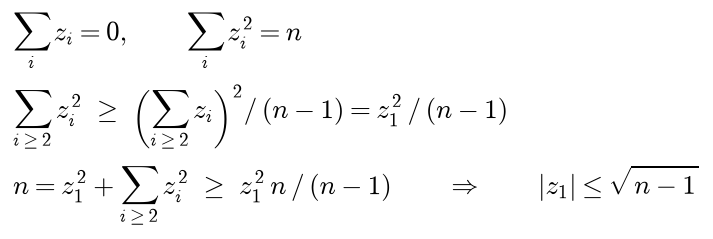
Equality holds exactly when all the other values are equal. This is Samuelson's inequality. With the sample standard deviation, the divisor n - 1, the same argument gives a bound of n - 1 divided by the square root of n. Either way, in a sample of ten or fewer values a three-sigma rule cannot flag anything, however extreme the value. In larger samples the effect weakens but does not vanish: several outliers inflate the standard deviation together and hide one another, which is called masking.

The median absolute deviation

The median and the MAD replace the mean and the standard deviation with statistics that up to half the data can corrupt without moving them arbitrarily far. Their breakdown point is 50 %, against 0 % for the mean and the standard deviation, which a single value can drag anywhere. For normal data, half of all values lie within one MAD of the median, which fixes the MAD as a multiple of the standard deviation, with Φ the standard normal distribution function:

The robust z-score therefore divides by the MAD scaled by 1 / 0.6745 = 1.4826, so that the scaled MAD estimates the standard deviation on normal data:

A cut-off of 3.5 on the absolute robust z-score, suggested by Iglewicz and Hoaglin, is common.

Rolling-window features

A time series carries information that a single reading does not. All windows here are trailing, built only from readings up to the present, so the features can be computed online and cannot leak the future into an evaluation. Three features are used:

• The residual ρ from a trailing median, divided by the scaled MAD of the residuals in the training period. The current reading is excluded from its own baseline.
• The rolling spread, the standard deviation of the last w readings divided by its typical value in training, on a log scale. A stuck sensor drives it to zero.
• The time of day as a point on the unit circle, so that 23:50 and 00:10 are neighbours. This is the context that contextual anomalies need.

The residual compares each reading with a baseline that does not contain it. The time of day becomes two coordinates, computed from the hour of the reading:

How the residual responds to the two shapes of fault follows directly from its definition. A spike of height A on top of a smooth signal is not in its own window, so the residual sees it at full height, about A. A linear drift of slope β per reading drags the median of the previous w readings along, half a window behind:

The residual stays at that constant for as long as the drift lasts, however large the drift becomes. With w = 12 and the pump's drift of 0.0559 °C per reading, that is 0.3636 °C, against a typical residual of 1.5379 °C. A global z-score, in contrast, grows with the total drift since its start and crosses its threshold once the reading leaves the normal range.

Isolation trees

An isolation tree is grown on a subsample of ψ readings. A node becomes a leaf that remembers how many readings reached it if its depth has reached the height limit, if it holds at most one reading, or if all its readings are identical. Otherwise it picks a feature uniformly among the features that are not constant at the node, draws a split value uniformly between the smallest and the largest value of that feature there, and sends the readings at or below the split value to the left child and the rest to the right child. The height limit is about the depth of a balanced tree on ψ points:

Paths longer than that belong to normal points, and their exact length does not matter. The path length of a reading counts the edges d(x) from the root to the leaf the reading reaches. When that leaf still holds m > 1 training readings, the tree stopped before isolating them, and c(m), the average number of further splits a full tree would have needed, is added:

For a leaf holding a single reading c(1) = 0, so the path length is just the depth.

The normalizer c(n)

c(n) is the average path length in a tree grown on n points, and it can be derived exactly in one setting. Take n evenly spaced points on a line. The split value is uniform between the smallest and the largest point, so it falls in each of the n - 1 equal gaps with probability 1 / (n - 1), leaving k points on the left and n - k on the right, and each side is again evenly spaced. Let S(n) be the expected sum of the depths of all n points in a fully grown tree, with S(1) = 0. The split adds one edge to the path of every point, which gives the first line below. Multiplying it by n - 1, writing the same equation for n + 1 and subtracting gives the second, and dividing by n (n + 1) the third:

The average depth c(n) = S(n) / n starts at c(1) = 0 and grows by 2 / (n + 1) at each step, so

where the last form uses H(n) = H(n - 1) + 1/n. It is the formula of the original paper, which obtains it from the equivalent problem of unsuccessful searches in a binary search tree. For other configurations the true mean depth differs, but c only has to set the scale. Growing 400 random trees per size on evenly spaced points gives, for example, a mean depth of 3.4250 for n = 8 against c(8) = 3.4357.

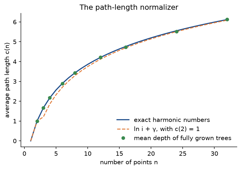
The simulated depths fall on the exact curve, while the approximation used by libraries sits visibly below it for the smallest sizes. That approximation replaces the harmonic number with a logarithm and Euler's constant γ:

It is accurate for large i but too small for small i: H(1) = 1 while ln 1 + γ = 0.5772. The approximate formula would give c(2) = 0.1544, so the original paper and scikit-learn define c(2) = 1 separately, and c(n) = 0 for n ≤ 1. With exact harmonic numbers no special case is needed. The two versions differ by less than 0.04 % at ψ = 256 (10.2487 against 10.2448) but noticeably for the small leaves where the correction is applied: c(3) = 1.6667 against 1.2074 and c(4) = 2.1667 against 1.8517. Our implementation uses exact harmonic numbers by default and the approximation when it reproduces scikit-learn.

The anomaly score

Path lengths grow with the subsample size, roughly like 2 ln ψ, so they are normalized by c(ψ) before being turned into a score:

The score approaches 1 as the expected path length shrinks towards zero, is exactly 0.5 when it equals c(ψ), and approaches 0 when the reading needs far more splits than average. Readings scoring well above 0.5 are candidates; if every reading scores about 0.5, the sample has no distinct anomalies. A reading needs at least one split, which caps the score:

The cap is 0.9346 for ψ = 256 and 0.8173 for ψ = 8. Growing T trees costs on the order of T ψ log ψ operations and scoring n readings n T log ψ, independent of the size of the training set. Small subsamples are a feature rather than a compromise. Swamping is the flagging of normal points that lie close to anomalies; masking is anomalies hiding one another when they are numerous or clustered. A large subsample contains a whole cluster of anomalies, which then looks like a small normal region, and both effects grow with ψ; a small subsample contains only a few of the clustered anomalies, which remain easy to isolate.

Reconstruction-error detectors

An autoencoder is a network trained to reproduce its input through a narrow middle layer. With the notation of Backpropagation, where W1 and b1 are the weights and biases of layer 1 and so on, the forward pass is the usual chain of layers ending in the reconstruction:

The network used on the pump has layers of 7, 16, 3, 16 and 7 units with tanh, identity, tanh and identity activations:

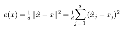
The amber bottleneck is the whole point: everything the network passes from its input to its output must squeeze through three numbers. The reconstruction error of a reading with d features is the mean squared difference between the reconstruction and the reading:

Training minimizes the mean of e(x) over the training readings with Adam. Only the output error differs from the general backpropagation recipe; the backward recursion through the layers and the parameter gradients are unchanged:

Three hidden units cannot copy seven inputs, so the network has to encode what the normal readings have in common: where in the daily cycle they are and how high the flow is, from which current, pressure, bearing temperature and vibration follow. A reading that breaks those relations, such as current too high for its flow or a bearing too warm for its current and time of day, is reconstructed as the normal reading closest to it, and the difference shows up in e(x).

The inputs are standardized with the mean and standard deviation of the training period, so roughly half of every feature is negative. The output layer must be able to produce such values, which makes it linear. A sigmoid output can only produce values between 0 and 1; the best it can do for a feature value x is to return x clipped to that interval, so its error per feature is at least the expected squared distance from x to the interval. For a standard normal feature, with φ the standard normal density, that floor is

an error floor far above what a linear output reaches on the same data.

Choosing a threshold

A threshold on any score can be chosen in several ways, all on data the final evaluation does not see:

• The (1 - α) quantile of the scores of normal validation readings fixes the false-alarm rate at about α. Every detector on the pump gets its threshold this way, with α = 1 %.
• The value that maximizes F1 on a labelled validation period uses the labels as well.
• The mean plus k standard deviations of the training errors assumes the errors are clean and roughly normal. They are skewed, and a few unlabelled faults in the training data inflate the standard deviation enormously.
• The median plus k scaled MADs of the training errors is the robust version of the previous rule and needs no labels at all.

Evaluation against labels

With TP, FP and FN the numbers of flagged anomalies, flagged normal readings and missed anomalies, precision is the share of flags that are right, recall the share of anomalies flagged, and F1 their harmonic mean:

Sweeping the threshold down through the distinct scores traces the precision-recall curve, and average precision summarizes it as the precision at each threshold weighted by the recall gained there:

A ranking that ignores the data has an expected average precision equal to the share of anomalies, which is the baseline to beat. Under heavy imbalance the ROC curve looks good for detectors that are useless in practice, while precision exposes them; Evaluation metrics explains why. Each reading counts once here. For anomalies that last, such as a stuck sensor or a drift, an operator cares about when an alarm is raised rather than about the share of readings flagged. The sample project therefore also reports, for every injected event, the delay until an alarm, defined as three consecutive flagged readings inside the event, or the flagged reading of an event shorter than that.

Contamination

Many libraries let the user set a contamination α and then put the threshold at the (1 - α) quantile of the scores of the training data. With linear interpolation that quantile lies at position (n - 1)(1 - α) of the n sorted scores, so whenever that position is not an integer, the number of training readings above it is

The number of flags is decided before the detector has looked at the data. With k true anomalies among the readings, recall cannot exceed the number of flags divided by k, and precision cannot exceed k divided by the number of flags. The arithmetic is the same as the false-alarm rule above; the difference is the sample. A quantile of normal validation readings fixes the false alarms, a quantile of all readings fixes the total.

Worked example

Ten vibration readings

Ten vibration readings in mm/s, the last one a spike: 2.1, 2.3, 1.9, 2.2, 2.0, 2.4, 2.1, 1.8, 2.2 and 6.0.

• They sum to 25.0, so the mean is 2.5.
• The deviations from the mean are -0.4, -0.2, -0.6, -0.3, -0.5, -0.1, -0.4, -0.7, -0.3 and 3.5. Their squares sum to 13.9, of which the spike alone contributes 12.25.
• The population variance is 1.39 and the standard deviation 1.1790.

No reading in a sample of ten can reach 3. With the sample standard deviation, the square root of 13.9 / 9, which is 1.2428, the z-score is 2.8163, under its own bound of 9 divided by the square root of 10, 2.8460.

Sorted, the readings are 1.8, 1.9, 2.0, 2.1, 2.1, 2.2, 2.2, 2.3, 2.4 and 6.0, and the median is the mean of the fifth and sixth, 2.15. The absolute deviations from the median, sorted, are 0.05, 0.05, 0.05, 0.05, 0.15, 0.15, 0.25, 0.25, 0.35 and 3.85, so the MAD is 0.15 and the scaled MAD 1.4826 × 0.15 = 0.2224.

That is far beyond any cut-off, while the lowest normal reading, 1.8, gets a robust z-score of -1.5738.

One isolation tree

Eight readings of bearing temperature (°C) and vibration (mm/s); P8 runs hot:

• P1 (20.0, 2.0), P2 (21.0, 2.4), P3 (22.0, 2.2), P4 (21.5, 1.8),
• P5 (20.5, 2.6), P6 (22.5, 2.1), P7 (21.0, 2.0), P8 (27.0, 2.3).

The height limit is the base-2 logarithm of 8, which is 3. Instead of random numbers, the tree uses four fixed draws, each a feature and a fraction u, consumed in the order the nodes are grown: a node, then its whole left subtree, then its right subtree. The split value is the smallest value at the node plus u times the range there.

• Root, all eight readings: temperature with u = 0.8. The range is 20.0 to 27.0, so the split value is 20.0 + 0.8 × 7.0 = 25.6. P1 to P7 go left and P8 right.
• Node A, P1 to P7: vibration with u = 0.55. The range is 1.8 to 2.6, so the split value is 1.8 + 0.55 × 0.8 = 2.24. P1, P3, P4, P6 and P7 go left, P2 and P5 right.
• Node B, P1, P3, P4, P6 and P7: temperature with u = 0.2. The range is 20.0 to 22.5, so the split value is 20.0 + 0.2 × 2.5 = 20.5. P1 goes left, P3, P4, P6 and P7 right.
• Node C, P2 and P5: temperature with u = 0.5. The range is 20.5 to 21.0, so the split value is 20.75. P5 goes left and P2 right.

The right child of B sits at depth 3, the height limit, so it becomes a leaf holding four readings and needs no draw.

The tree isolates the hot reading with its first cut, while the readings in the dense middle of the data share a leaf at the height limit. The normalizers come from the harmonic numbers H(3) = 1 + 1/2 + 1/3 = 1.8333 and H(7) = 2.5929:

The path lengths and single-tree scores, with the score 2 to the power minus h / c(8):

• P8 is isolated by the first split: h = 1, h / c(8) = 0.2911, score 0.8173.
• P1, P2 and P5 end alone at depth 3: h = 3, h / c(8) = 0.8732, score 0.5459.
• P3, P4, P6 and P7 share a leaf at the height limit: h = 3 + c(4) = 5.1667, h / c(8) = 1.5038, score 0.3526.

One tree is one random draw; a forest averages h over many. With 100 random trees, each grown on all eight readings (ψ = 8, seed 0), the expected path lengths and scores are:

• P1: E[h] = 3.7823, score 0.4662. P2: 3.9713, 0.4488. P3: 4.3167, 0.4186. P4: 3.5723, 0.4864.
• P5: E[h] = 2.9060, score 0.5564. P6: 4.2187, 0.4269. P7: 4.6313, 0.3928. P8: 2.2697, 0.6326.

P8 scores highest and P5, the reading with the highest vibration, second. No score can exceed the single-tree score of P8, 0.8173, because no reading can be isolated in fewer than one split. With the logarithmic approximation of the harmonic numbers the normalizers would be c(4) = 1.8517 and c(8) = 3.2963.

Precision, recall and average precision

A detector ranks ten readings with the scores 0.81, 0.74, 0.69, 0.62, 0.58, 0.55, 0.51, 0.47, 0.44 and 0.40; the first, third and fifth are real anomalies.

• The threshold 0.6 flags the top four: TP = 2, FP = 2 and FN = 1, so the precision is 0.5, the recall 0.6667 and F1 = 2 × 0.5 × 0.6667 / 1.1667 = 0.5714.
• Lowering the threshold one score at a time gives the precision and recall pairs (1, 0.3333), (0.5, 0.3333), (0.6667, 0.6667), (0.5, 0.6667), (0.6, 1), and then precision falling to 0.3 at recall 1.
• Recall rises at the first, third and fifth readings, by a third each time.

Against that 0.7556, a ranking that ignores the data scores 0.3 on average. The best F1, 0.75, is reached at the threshold 0.58 with precision 0.6 and recall 1. A contamination of α = 0.2 puts the threshold at position 0.8 × 9 = 7.2 of the scores sorted upwards, 0.69 + 0.2 × (0.74 - 0.69) = 0.70, and flags the ceiling of 0.2 × 9, which is 2 readings, whatever the labels.

A reconstruction error and two thresholds

A standardized reading with three features, x = (0.8, -1.2, 0.5), and its reconstruction x̂ = (0.5, -0.8, 0.6):

A sigmoid output could at best return (0.8, 0, 0.5), an error of one third of 1.2 squared, 0.48, from the negative feature alone. Ten normal validation readings have the errors 0.021, 0.034, 0.018, 0.027, 0.045, 0.030, 0.024, 0.039, 0.016 and 0.052.

• Their mean is 0.0306 and their standard deviation 0.0113, so the mean plus three standard deviations is 0.0644.
• The 90th percentile lies at position 0.9 × 9 = 8.1 of the sorted errors, 0.045 + 0.1 × (0.052 - 0.045) = 0.0457.

The reading's error of 0.0867 exceeds both thresholds, so it is flagged either way; a sigmoid output would have pushed every reading with a negative feature above both. Every number in this section is asserted by tests/test_worked_example.py and printed by examples/worked_example.py.

The code

The package anomaly_detection is plain NumPy, split into one module per idea. scikit-learn and PyTorch are imported only inside the functions of comparisons.py and the contamination study, so everything else works without them.

• arrays.py holds the array types and as_points, which insists on one reading per row.
• baselines.py holds z_scores, median_absolute_deviation and robust_z_scores, each with an optional reference sample so statistics fitted on training data can score new data, and samuelson_bound.
• windows.py holds the trailing windows, which are NaN until enough history exists and can exclude the current reading, the rolling mean, median, spread and residual, and the time-of-day features.
• path_length.py holds harmonic_number and average_path_length with exact or logarithmic harmonic numbers, anomaly_score, and the wrong mixed_normalizer for the Pitfalls section.
• isolation_tree.py holds IsolationTree, a frozen class of node arrays, the random and scripted splitters, grow_isolation_tree and the simulation of mean depths behind c(n).
• isolation_forest.py holds IsolationForest and fit_isolation_forest.
• thresholds.py holds the contamination, quantile, three-sigma and robust threshold rules and flag.
• metrics.py holds the confusion counts, precision, recall and F1, the precision-recall curve with ties handled as one point, average precision, the best-F1 threshold and a rank correlation.
• alarms.py turns flags into alarms: alarm_index for a run of consecutive flags, recall_by_kind and event_delays.
• activations.py, autoencoder.py, training.py and gradient_check.py hold the autoencoder: the activation functions, the Autoencoder class with its backpropagation gradients, Adam training that performs the same floating-point operations as torch.optim.Adam, and a central-difference gradient check.
• pump.py simulates the pump with its injected faults; datasets.py generates the point clouds for the Isolation Forest demonstrations.
• monitor.py runs the seven detectors on the pump and calibrates their thresholds; evaluation.py scores a run against the labels and reports.py formats the results as text.
• forest_pitfalls.py and pump_pitfalls.py hold the experiments behind the Pitfalls section.
• worked_example.py holds the numbers of the worked example, comparisons.py the bridges to scikit-learn and PyTorch, and plotting.py, forest_plots.py and pump_plots.py draw every figure in the handbook's four colours.

A tree is stored as parallel arrays, one entry per node, with a feature of -1 marking a leaf, so scoring loops over depth rather than over readings. Every reading that has not reached a leaf moves one level down at a time, and path_lengths then adds c of the leaf size to the depth:

node = np.zeros(points.shape[0], dtype=np.int64)
depth = np.zeros(points.shape[0], dtype=np.int64)
active = np.flatnonzero(self.feature[node] != LEAF)
while active.size:
    current = node[active]
    goes_left = points[active, self.feature[current]] <= self.threshold[current]
    node[active] = np.where(goes_left, self.left[current], self.right[current])
    depth[active] += 1
    active = active[self.feature[node[active]] != LEAF]

Growing a tree takes a splitter, a function from the readings at a node to a feature and a split value. random_splitter draws them as the method prescribes; scripted_splitter replays given draws, which is how hand_tree builds the worked example's tree.

The examples and the project import the package, so install the repository first as described in the main README. Each example demonstrates one idea and runs in a few seconds from the repository root:

• examples/worked_example.py prints every value of the worked example in the order above.
• examples/path_length_normalizer.py checks c(n) against its recursion and against the mean depth of random trees, compares the logarithmic approximation and saves the plot shown under How it works.
• examples/subsample_size.py measures swamping and masking of a dense cluster of anomalies for subsample sizes from 16 to 2048 and saves the figure shown under Pitfalls.
• examples/fixed_contamination.py shows a contamination setting fixing the number of flags on seven batches and saves the figure shown under Pitfalls.
• examples/common_mistakes.py demonstrates the pitfalls without a figure of their own, from Samuelson's bound to a threshold tuned on the test period.
• examples/compare_with_libraries.py compares our forest with scikit-learn's, our precision-recall curve with sklearn.metrics and our autoencoder with PyTorch, and saves the score maps shown under In practice.

python machine-learning/anomaly-detection/examples/worked_example.py
python machine-learning/anomaly-detection/examples/path_length_normalizer.py
python machine-learning/anomaly-detection/examples/subsample_size.py
python machine-learning/anomaly-detection/examples/fixed_contamination.py
python machine-learning/anomaly-detection/examples/common_mistakes.py
python machine-learning/anomaly-detection/examples/compare_with_libraries.py

The sample project: monitoring a pump

project/sensor_monitor.py applies everything to a month of sensor data. It simulates the pump, scores every reading with seven detectors, calibrates each detector's threshold on the validation period at a fixed false-alarm rate, and reports precision, recall, average precision, the recall for each kind of fault, five threshold rules for the autoencoder, and how long each detector takes to raise an alarm for each injected event. The default run takes under three seconds.

The periods are split by time, never at random, and nothing about the test period enters any choice. make_pump_data simulates a water pump read every ten minutes for 30 days. Demand follows a daily cycle with its low at 05:00 and its peak at 17:00; flow follows demand with slowly varying noise; the motor current rises with flow and the outlet pressure falls with it; the bearing temperature follows the ambient temperature and the current; and vibration rises slightly with flow. Day 0 fills the rolling windows; days 1 to 13 are for training (1872 readings, 84 anomalous), days 14 to 19 for validation (864, 83) and days 20 to 29 for testing (1440, 235). The injected faults are 18 spikes of 2.5 to 6 standard deviations, four one-hour night leaks, three six-hour stuck sensors, three six-hour periods of current 0.6 A too high for the flow, and an 8 °C drift of the bearing temperature over the last day. The training period contains faults too, as real training data would, and nobody tells the detectors where.

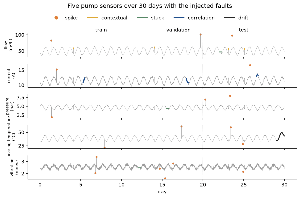
Most faults are invisible at this scale, which is the point: only the spikes and the end of the drift stand out from the daily cycle. The seven detectors are:

• z-score: the largest absolute z-score over the five sensors, with the mean and standard deviation of the training period.
• MAD: the largest absolute robust z-score, with the median and MAD of the training period.
• rolling residual: the largest residual from the median of the previous two hours, divided by its typical size in training.
• rolling spread: the largest drop of the log one-hour standard deviation below its typical training value.
• forest, sensors: our Isolation Forest on the five readings, 100 trees on subsamples of 256 from the training period.
• forest, sensors and time: the same with the two time-of-day coordinates added.
• autoencoder: the reconstruction error of the 7-16-3-16-7 network, trained for 150 epochs with Adam on the standardized training readings and the time of day.

On the test period, where 16.3 % of the readings are anomalous, the average precision, precision, recall and F1 at the calibrated thresholds are:

• z-score: AP 0.513, precision 0.774, recall 0.277, F1 0.408.
• MAD: AP 0.398, precision 0.627, recall 0.136, F1 0.224.
• rolling residual: AP 0.263, precision 0.500, recall 0.094, F1 0.158.
• rolling spread: AP 0.361, precision 0.607, recall 0.145, F1 0.234.
• forest, sensors: AP 0.402, precision 0.408, recall 0.085, F1 0.141.
• forest, sensors and time: AP 0.459, precision 0.560, recall 0.119, F1 0.196.
• autoencoder: AP 0.936, precision 0.927, recall 0.864, F1 0.894.

Each baseline catches what it was built for and little else. The global scores catch every test spike; the rolling residual catches the spikes and the night leaks, which are short enough to be a jump relative to the previous two hours; the rolling spread catches 86 % of the stuck sensor's readings, all but its first 50 minutes, and almost nothing else; adding the time of day lets the forest catch every night leak. The autoencoder sees how the sensors relate to each other and to the time of day, so it is the only detector that catches all of the correlation break and most of the drift and of the stuck sensor: it flags 86 % of the spike readings, all of the leak and correlation-break readings, 89 % of the stuck readings and 81 % of the drift readings. The z-score and the forest on sensors catch only the 39 % of the correlation break between 15:00 and 18:00, around the demand peak, where the extra 0.6 A lifts the current above anything seen in training.

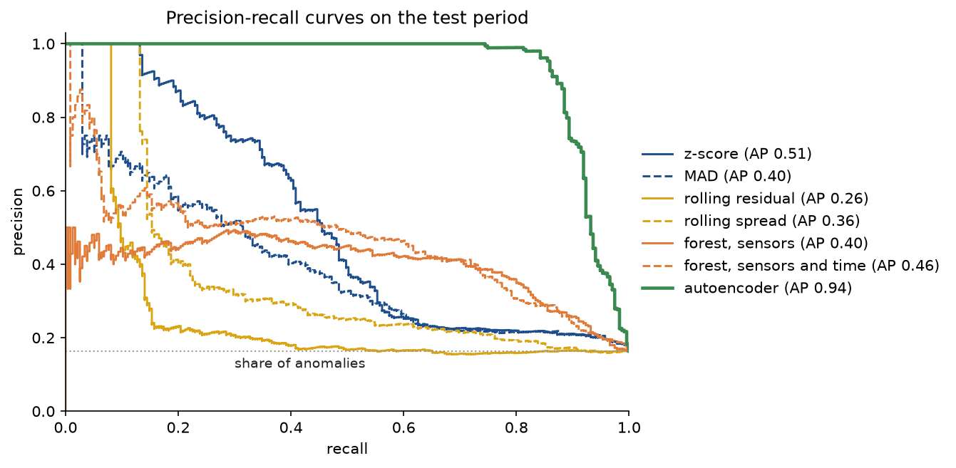
The autoencoder's curve dominates everywhere; the others trade a little precision at low recall for nothing at high recall, where they sink to the share of anomalies.

The threshold matters as much as the score. Five rules for the autoencoder's errors, each with its threshold and its precision, recall and F1 on the validation and test periods:

• 1 % of normal validation errors: threshold 0.0146; validation 0.902, 0.892 and 0.897; test 0.927, 0.864 and 0.894.
• Best F1 on the labelled validation period: 0.0177; validation 0.961, 0.880 and 0.918; test 0.980, 0.838 and 0.904.
• Median plus 3 scaled MADs of the training errors: 0.0099; validation 0.664, 0.928 and 0.774; test 0.784, 0.894 and 0.835.
• Mean plus 3 standard deviations of the training errors: 0.1733; validation 1.000, 0.036 and 0.070; test 1.000, 0.247 and 0.396.
• Top 1 % of all validation readings: 0.0947; validation 1.000, 0.108 and 0.196; test 1.000, 0.328 and 0.494.

The two rules that use validation data agree; the robust training rule needs no labels at all and loses only some precision; the last two rules are pitfalls described below.

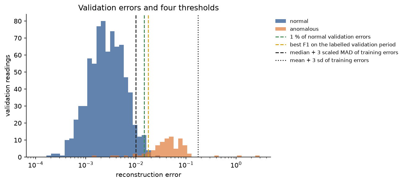
The normal and anomalous errors overlap only in a narrow band around 0.01 to 0.03, which is where every sensible threshold lands; the three-sigma rule on contaminated errors lands an order of magnitude to the right.

Spikes and drift, at the same calibrated thresholds. A spike counts as caught when its reading is flagged, in the validation and test periods together; the drift alarm is the first moment three consecutive readings are flagged, so that isolated false alarms inside the drift do not count:

• z-score: 10 of 12 spikes; 31 % of the drift readings flagged; alarm after 13.00 hours, when the drift has added 4.36 °C.
• MAD: 10 of 12 spikes; 17 % of the drift; alarm after 14.17 hours, at 4.76 °C.
• rolling residual: 12 of 12 spikes; 1 % of the drift; no alarm.
• rolling spread: no spikes; 1 % of the drift; no alarm.
• forest, sensors: 6 of 12 spikes; 2 % of the drift; no alarm.
• forest, sensors and time: 5 of 12 spikes; 3 % of the drift; no alarm.
• autoencoder: 11 of 12 spikes; 81 % of the drift; alarm after 5.00 hours, at 1.68 °C.

This is the behaviour the mathematics predicted. The rolling residual sees every spike at full height and the drift as a constant offset of about 0.37 °C, well inside its normal range. The global scores catch spikes that leave the normal range and the drift only after 13 hours, when it has added more than 4 °C and pushed the afternoon readings out of the range. The forests never raise the alarm, because a tree sends every reading beyond the training maximum to the same leaf as that maximum (see Pitfalls). The autoencoder raises it after five hours, at 1.7 °C.

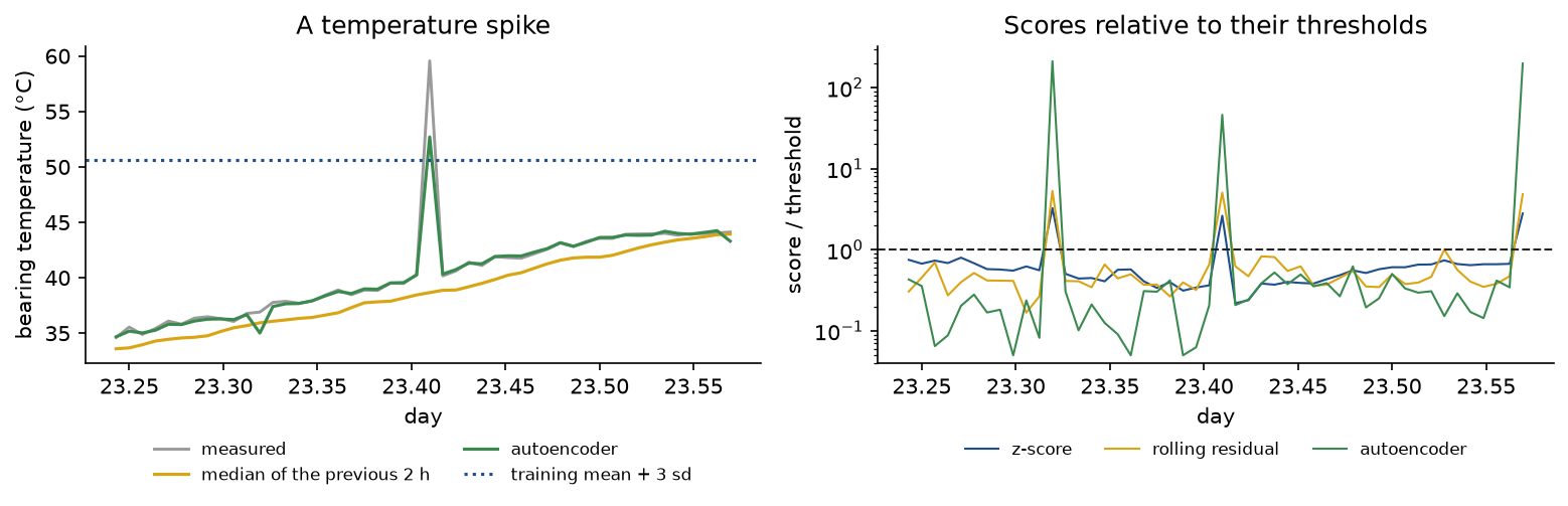
At the temperature spike all three detectors cross their thresholds: the z-score by a factor of 2.6, the rolling residual by 5.1 and the autoencoder by 46. The two other peaks in the right panel belong to spikes of the pressure and the flow sensor in the same hours, which every detector sees because each score is the worst over the sensors.

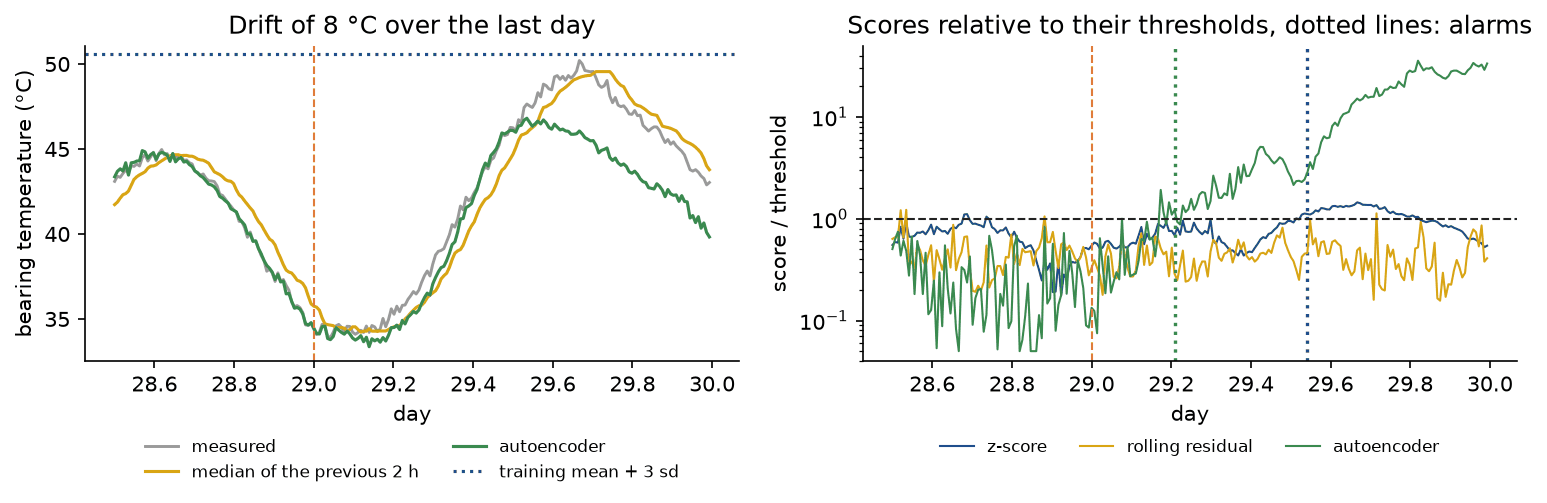
The trailing median follows the drift, so the residual never grows, while the reconstruction stays where a healthy bearing would be, and the gap between the two is the drift. The detection delays per test event tell the same story in operator terms. An event is detected when an alarm is raised inside it, and the delay counts from the start of the event:

• autoencoder: 6 of 7 spikes; both night leaks after 20 minutes, the earliest a run of three flags can complete; the stuck sensor after 60 minutes; the correlation break after 20 minutes; the drift after 300 minutes.
• z-score: all 7 spikes; the correlation break after 210 minutes, once the demand peak lifts the current out of range; the drift after 780 minutes; neither the leaks nor the stuck sensor.
• rolling residual: all 7 spikes and both leaks after 20 minutes; nothing else.
• rolling spread: only the stuck sensor, after 70 minutes.
• forests: 3 and 2 of the 7 spikes, the correlation break after 190 and 210 minutes, the leaks after 20 minutes once the time of day is added, and never the drift.

Options such as --drift, --false-alarm-rate, --alarm-run, --trees, --subsample-size, --epochs and the three seeds change the setup, and --figures sends the five PNGs to another folder so a custom run does not overwrite the ones shown here. With a drift of only 2 °C (--drift 2), no detector but the autoencoder ever raises the drift alarm, and the autoencoder does so after 14 hours, at 1.17 °C.

python machine-learning/anomaly-detection/project/sensor_monitor.py
python machine-learning/anomaly-detection/project/sensor_monitor.py --drift 2 --figures pump-figures

The notebook anomaly_detection.ipynb is a guided tour in the order of this page: the worked example, the normalizer, score maps, the autoencoder's gradients, the pump run with every detector, a demonstration of each pitfall, and the library comparisons. The tests in tests check the worked example value by value, the mathematical properties above, the pump results quoted here and the agreement with scikit-learn and PyTorch, and run in under ten seconds:

python -m pytest machine-learning/anomaly-detection

Every dataset is synthetic and generated from a seed by make_pump_data, make_scattered_outliers, make_cluster_data and make_contaminated_batch, so nothing is downloaded and no licence applies.

In practice

scikit-learn's IsolationForest

sklearn.ensemble.IsolationForest implements the same method with 100 trees, subsamples of at most 256 readings by default and the same height limit. Our forest and scikit-learn's draw different random trees, so they are compared in two ways. Applied to scikit-learn's own fitted trees, our path lengths, leaf correction and normalizer, with the logarithmic harmonic numbers scikit-learn uses, reproduce its scores to within 4 × 10⁻¹⁶ (score_with_sklearn_trees, tested in tests/test_comparisons.py). scikit-learn compares features in single precision, so the readings are cast to float32 before routing them. Independently grown forests can only agree in their rankings: on two clusters with ten scattered outliers, the rank correlation between our scores and scikit-learn's over a grid of the plane is 0.9887, and between two scikit-learn forests with different seeds 0.9869.

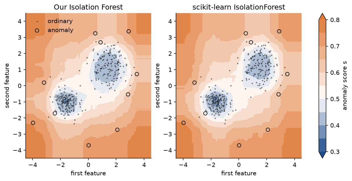
The maps are alike rather than identical, as two random forests must be. The bands parallel to the axes are a property of the method, which only ever splits along one coordinate.

Mind the conventions. score_samples returns minus s, the negative of the paper's score, so larger means more normal; decision_function subtracts offset_ from it; and predict returns -1 for flagged readings and +1 otherwise. With contamination="auto" the offset is -0.5 and the cut is s > 0.5: on the two clusters, predict and s > 0.5 both flag 47 of the 310 points. With a number, the cut is the contamination quantile of the training scores (see Pitfalls).

On the pump, scikit-learn's forest on the same sensors and time of day reaches a test average precision of 0.478 against our 0.459. Their rank correlation on the test period is only 0.7421, because most test readings are ordinary and score close to each other, but two scikit-learn forests with different seeds agree even less, 0.6954. sklearn.metrics.precision_recall_curve and average_precision_score give exactly our curve, and the autoencoder's test average precision is 0.935874 in both; scikit-learn lists the thresholds upwards and appends a final point with precision 1 and recall 0, so sklearn_precision_recall reverses its output before comparing.

The autoencoder in PyTorch

The usual PyTorch version of the same model is an nn.Sequential of Linear, Tanh and Identity modules trained with torch.optim.Adam on the mean squared error over all entries, which is exactly our cost. The central-difference gradient check gives relative errors of 5.8 × 10⁻¹⁰ for a linear output and 3.4 × 10⁻⁹ for a sigmoid output, and autograd's gradients agree with ours to about 10⁻¹⁶. Started from the same weights and fed the same batches in the same order, the PyTorch run follows our loss curve to within 6 × 10⁻¹⁷ over 150 epochs on the pump, and its reconstruction errors differ from ours by at most 6 × 10⁻¹⁵, so its test average precision is the same 0.936.

When to use which

• z-scores and the MAD are a sanity check for one roughly stationary signal. Prefer the MAD, fit both on reference data rather than on the data being judged, and remove known cycles first: on the pump the daily cycle alone carries normal readings to absolute z-scores of about 2.
• Rolling residuals and spreads are cheap, explainable and good at spikes and stuck sensors; they are blind to drift by construction.
• An Isolation Forest is a strong default for tabular data without labels: fast, little tuning, no scaling needed. Give it only relevant features, add the context explicitly, keep the subsample small and do not let a contamination setting choose the threshold. scikit-learn's version is the one to use in practice; its max_samples is the subsample size.
• A reconstruction-error detector pays off when the sensors are correlated, which is when anomalies show up as broken relations rather than extreme values. It needs mostly normal training data, inputs standardized with training statistics, a linear output and a threshold chosen on validation data.
• Slow drift needs a change detector on top: a cumulative sum (CUSUM) of the autoencoder's error or of a residual from a long-run reference accumulates small persistent deviations that no per-reading threshold sees.

Other detectors worth knowing are the local outlier factor (sklearn.neighbors.LocalOutlierFactor, with novelty=True for new data), the one-class SVM and robust covariance (EllipticEnvelope). The Extended Isolation Forest replaces axis-parallel splits with random hyperplanes and removes the bands visible in the score maps. The Edge AI part takes a sensor autoencoder like this one to an int8 runtime on a device.

Pitfalls

• A fixed contamination fixes the number of flags. Cutting at the contamination quantile of the training scores flags the ceiling of α (n - 1) readings whatever the data contain. On seven batches of 1000 readings with 0 to 300 anomalies, refitting a forest on each batch with contamination 0.05, ours or scikit-learn's, flags exactly 50 every time: 50 false alarms on the clean batch, and a recall of 0.17 on the batch with 300 anomalies. A report that a detector "found 20 anomalies" in data with 20 injected ones says nothing when contamination was set to 20 out of the total; only a comparison with the labels does. contamination="auto" is no cure either: its cut s > 0.5 flags 206 of the 1000 clean readings. A forest fitted once on clean reference data, with its threshold frozen at a 1 % false-alarm rate, flags 5 readings on the clean batch and 238 on the batch with 300. examples/fixed_contamination.py prints the counts and draws the figure.

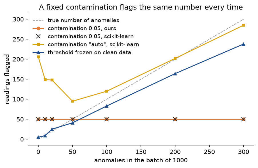
Only the frozen threshold tracks the truth; the contamination rule draws a horizontal line whatever the batch holds.

• Three-sigma rules on small or contaminated samples. By Samuelson's inequality no z-score in a sample of ten can exceed 3, so the rule cannot fire; the worked example's spike reaches 2.9687, and 1000 among nine zeros reaches exactly 3.0000. In larger samples outliers inflate the standard deviation and hide each other. Use the median and the MAD, or fit the statistics on clean reference data. examples/common_mistakes.py prints the bound and the attained value for 5, 10, 20 and 50 readings.
• Large subsamples cause swamping and masking. More data does not help an Isolation Forest. With 100 clustered anomalies among 2000 ordinary points, average precision is 0.998 at a subsample size of 16 and 0.193 at 2048, where 98 % of the anomalies score below the 99th percentile of the ordinary points and 194 ordinary points outscore the median anomaly. Very small subsamples cost something too: with 40 clustered anomalies the best size is 32 (average precision 0.989) and 16 gives 0.736. examples/subsample_size.py prints both sweeps.

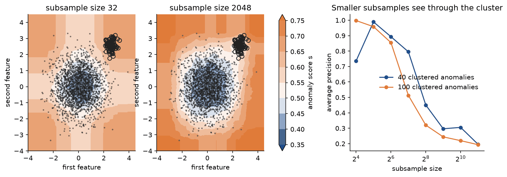
With a subsample of 32 the cluster sits in an orange region that is easy to isolate; with 2048 it is pale, as if it were a small normal region, while the edge of the main cloud turns orange.

• The normalizer with mixed sizes. Some write-ups put the number of points being scored into c, as below. Both places must hold the size of the sample each tree was grown on.

With the mixed form, the score of one reading with E[h] = 5 under ψ = 256 is 1.0935 when ten readings are scored together (c = -38.7591), 0.7442 for 1000 and 0.7533 for 100000, instead of 0.7131. A related subtlety is the logarithmic approximation of H, poor for the small leaf sizes where the correction is applied; it is harmless only because it is applied consistently. examples/common_mistakes.py prints these scores.

• A sigmoid output on standardized inputs. Half of every standardized feature is negative and a sigmoid cannot produce it. On the pump the error floor computed from the training inputs alone is 0.4583, the sigmoid network's training loss stops at 0.4610, the median error of normal validation readings is 0.3503 instead of 0.0025, and test average precision falls from 0.936 to 0.234. Use a linear output, or scale the inputs to the interval from 0 to 1 if a sigmoid output is really wanted. The notebook section "A sigmoid output on standardized inputs" plots both loss curves.
• Mean plus three standard deviations of contaminated errors. The pump's training errors have a median of 0.0029 and a maximum of 1.949, because the training period contains unlabelled faults. Their standard deviation is 0.0556, against 0.0034 without the faults, so the rule's threshold is 0.1733 and test recall 0.247. The median and MAD of the same errors give 0.0099 and an F1 of 0.835; removing the faults, which needs labels, gives 0.0139 and 0.890.
• Rolling windows absorb slow drift. A residual from a trailing baseline stays at β (w + 1) / 2 during a linear drift: 0.3680 °C measured against 0.3636 °C predicted on the pump, while the drift reaches 8 °C. Compare with a long-run reference, or with what the other sensors imply, to see drift. And never use centred windows: they need future readings, which an online detector does not have and which leak into an offline evaluation.
• Scores stop growing outside the training range. Split values lie within the training range, so every reading beyond the training maximum follows the same path as the maximum. A forest fitted on 1000 standard normal readings gives the maximum, 3.3230, and the readings 5, 10 and 1000 the same score, 0.7744. A forest therefore ranks an extreme reading no higher than a merely unusual one at the edge of the data, and a drift that leaves the range stops raising the score.
• Irrelevant features dilute an Isolation Forest. Each split uses one randomly chosen feature, so uninformative features waste splits. Adding ten rolling-window features to the pump forest on sensors and time of day lowers its test average precision from 0.459 to 0.301, although each of those features serves a dedicated detector well. Choose features per kind of anomaly, or use a detector that learns which matter.
• Choosing the threshold on the test data, or splitting a time series at random. A threshold tuned on the data it is evaluated on reports the best case, not the expected one. Choosing the best-F1 threshold on the validation period gives the z-score a test F1 of 0.357; tuning it on the test period itself reports 0.493. The gap is small only for a detector that is good anyway: 0.904 against 0.906 for the autoencoder. A random split of a time series puts neighbours of every test reading into training, where rolling features and the model have already seen them. Split by time, as the pump's periods are, and tune on the validation period only; Data leakage and pitfalls collects more of these.
• Reading scikit-learn's signs the wrong way round. score_samples is minus s and predict returns -1 for anomalies. Sorting by score_samples in decreasing order ranks the most normal readings first, which turns a good detector into an apparently terrible one: on the two clusters with ten outliers, average precision falls from 0.862 to 0.018. examples/compare_with_libraries.py prints both.

Further reading

• F. T. Liu, K. M. Ting and Z.-H. Zhou, "Isolation forest", Proceedings of the IEEE International Conference on Data Mining, 413-422, 2008. The method, the score and the role of subsampling.
• F. T. Liu, K. M. Ting and Z.-H. Zhou, "Isolation-based anomaly detection", ACM Transactions on Knowledge Discovery from Data 6(1), 3:1-3:39, 2012. The extended version with swamping, masking and the height limit analysed.
• S. Hariri, M. Carrasco Kind and R. J. Brunner, "Extended isolation forest", IEEE Transactions on Knowledge and Data Engineering 33(4), 1479-1489, 2021.
• V. Chandola, A. Banerjee and V. Kumar, "Anomaly detection: a survey", ACM Computing Surveys 41(3), 15:1-15:58, 2009. The point, contextual and collective taxonomy.
• P. A. Samuelson, "How deviant can you be?", Journal of the American Statistical Association 63(324), 1522-1525, 1968.
• B. Iglewicz and D. C. Hoaglin, How to Detect and Handle Outliers, ASQC Quality Press, 1993. Modified z-scores and the 3.5 cut-off.
• P. J. Rousseeuw and C. Croux, "Alternatives to the median absolute deviation", Journal of the American Statistical Association 88(424), 1273-1283, 1993.
• D. E. Knuth, The Art of Computer Programming, volume 3, second edition, section 6.2.2, Addison-Wesley, 1998. Path lengths of random binary search trees.
• M. Sakurada and T. Yairi, "Anomaly detection using autoencoders with nonlinear dimensionality reduction", Proceedings of the MLSDA Workshop, 4-11, 2014.
• E. S. Page, "Continuous inspection schemes", Biometrika 41(1-2), 100-115, 1954. The CUSUM change detector.
• T. Saito and M. Rehmsmeier, "The precision-recall plot is more informative than the ROC plot when evaluating binary classifiers on imbalanced datasets", PLoS ONE 10(3), e0118432, 2015.
• S. Kim, K. Choi, H.-S. Choi, B. Lee and S. Yoon, "Towards a rigorous evaluation of time-series anomaly detection", Proceedings of the AAAI Conference on Artificial Intelligence 36(7), 7194-7201, 2022. How common evaluation protocols inflate time-series results.