Loss functions

Training sees the data only through the gradient of the loss, so the loss decides two things at once: what the trained model predicts (the mean, the median, a quantile or a probability) and how fast and how robustly it gets there. Pick squared error for a sigmoid classifier and a confidently wrong output barely learns; pick cross-entropy and a few mislabelled points can drag the decision boundary across the data; use the wrong library convention and the gradient is off by a factor nobody notices. This page derives the common losses as negative log-likelihoods of noise models, shows why each output activation has a matching loss whose output error is simply a - y, and measures the learning slowdown of a saturated sigmoid in a one-neuron experiment from two starting points. It then works through softmax and its Jacobian, numerically stable log-softmax, label smoothing, class weights and focal loss for imbalanced data, the Huber and pinball losses for regression, the hinge for comparison, and contrastive and triplet losses in brief. A sample project fits the same line to glitchy sensor readings under four losses and trains a rare-event classifier with class weights, a moved threshold and focal loss. Every loss is implemented in NumPy and checked against its torch.nn counterpart. Afterwards you will be able to choose a loss from what you know about the targets and the noise, derive its gradient, compute it without overflow, and predict how it will treat outliers, mislabelled points and rare classes. It builds on Backpropagation.

To run the code in this topic, install the base group, the deep group for the comparisons with PyTorch, and the ml group for the exact solvers from SciPy and scikit-learn.

Intuition

A loss turns "how wrong is this prediction" into a number, and gradient descent follows the derivative of that number. Two questions about a loss tell you almost everything about the model it trains.

• Where is it smallest? If a model could output only one constant, squared error would pick the mean of the targets, absolute error the median, the pinball loss a quantile, and cross-entropy the frequency of each class. A network trained with a loss estimates that same statistic of the target given the input. Choosing a loss is therefore choosing what to predict.
• How does its gradient behave away from the minimum? The gradient with respect to the output is the force with which each example pulls on the parameters. Under squared error that force grows with the residual, so a single outlier can dominate; under the Huber loss it is capped; under a bounded loss it fades to nothing for examples that are badly wrong. The same fading is what stalls a saturated sigmoid output under squared error: the neuron is maximally wrong and learns slowly because its output barely responds to its net input.

Most standard losses are not arbitrary choices. Each is the negative log-likelihood of a noise model, and pairing it with the output activation that turns the net input into that model's mean makes the output error collapse to prediction minus target.

Each row reads from left to right: the noise model, the loss that is its negative logarithm, the output activation that matches it, and the output error that results. Three of the four rows meet in the same green box, and that shared result, δ = a - y, is the reason these pairs are used together.

How it works

Notation

The notation is that of Backpropagation. Only the output layer matters on this page, so z, a and δ stand for the net input, the activation and the error of the output layer, which that page writes with a superscript (L); the formula images here drop the superscript.

• x is one input and y its target. For K classes, y is a one-hot or probability vector and c is the true class.
• z is the net input of the output layer, called the logits for a classifier, and a = f(z) is the output of the network.
• C is the cost of one example. The cost of a mini-batch of m examples is the average of the per-example costs.
• δ is the output error, the derivative of C with respect to z, equation B1 of backpropagation.
• σ is the sigmoid, whose derivative is σ′(z) = σ(z)(1 - σ(z)) = a(1 - a).
• LSE(z) is log-sum-exp, the logarithm of the sum of the exponentials of the logits.
• r = y - ŷ is the residual of a regression prediction ŷ.
• t = 2y - 1 is a binary label written as plus or minus one, and t z is the margin.
• [P] is 1 if the statement P is true and 0 otherwise.

Losses as negative log-likelihoods

Suppose the network's output is the parameter of a probability distribution for the target, p(y | x; θ), where θ holds all weights and biases. For independent examples the likelihood is a product, its logarithm a sum, and maximizing it is the same as minimizing the average negative log-likelihood. The cost of one example is therefore

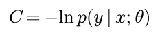
with any additive constant and any positive factor that does not depend on θ dropped, since neither moves the minimum. Four noise models give the four standard losses.

Gaussian noise. If each of the n targets is the output plus independent Gaussian noise of standard deviation s, the density and its negative logarithm are

For a fixed s this is the squared-error cost, one half the squared distance between output and target, up to a factor and a constant. If the network also predicts the variance v of each output, the logarithm stays in the cost, and the result is PyTorch's GaussianNLLLoss:

A large predicted variance excuses a large residual, but the log v term charges for it, so the network learns how noisy each prediction is.

Laplace noise. The Laplace density has heavier tails than the Gaussian, so large residuals are less surprising and cost less:

Its negative log-likelihood is the absolute error, scaled by 1/s.

Bernoulli label. For y in {0, 1} and a = P(y = 1 | x), exactly one of the two exponents below is 1, and the negative logarithm is the binary cross-entropy:

Categorical label. For K classes with a_k the probability of class k and a one-hot y, the product picks out the probability of the true class:

The name cross-entropy comes from information theory. For a target distribution q and a predicted distribution p, the cross-entropy splits into the entropy of q and the Kullback-Leibler divergence from q to p:

The entropy of q does not depend on the parameters, so minimizing the cross-entropy minimizes the divergence from the targets to the predictions. The same formula therefore makes sense for soft targets, any y with nonnegative entries summing to one (Information theory).

What each loss estimates. Let a model output one constant ŷ for targets y1 to yn and set the derivative of the total loss to zero:

The derivative of the absolute error exists only away from the data points, and it changes sign where half the targets lie on each side. With inputs, the same arguments hold for each x separately: a flexible enough model trained with squared error predicts the conditional mean of y given x, with absolute error the conditional median, and with cross-entropy the conditional probability. Losses whose minimizer is the true probability are called proper scoring rules; cross-entropy and the squared error on probabilities (the Brier score) are proper, and the focal loss and the hinge below are not.

In short, the four rows of the diagram under Intuition are:

• Gaussian noise: cost one half (a - y) squared, identity output, output error a - y, best constant the mean.
• Laplace noise: cost the absolute value of a - y, identity output, output error the sign of a - y, best constant the median.
• Bernoulli label: binary cross-entropy, sigmoid output, output error a - y, best constant the frequency of the label 1.
• Categorical label: softmax cross-entropy, softmax output, output error a - y, best constants the class frequencies.

Why the matching pairs give a - y

Three of the four models belong to the exponential family, densities of the form below, where η is the natural parameter and A, the log-partition function, makes the density integrate to one:

The second statement follows by differentiating the condition that the density integrates to one under the integral sign. If the net input is the natural parameter, z = η, the cost and the output error are

Defining the output as the mean, a = ∇A(z), makes δ = a - y exactly. Reading off A for each model gives the matching output activation:

The sigmoid and the softmax are therefore not arbitrary squashing functions: they are the inverse canonical links of the Bernoulli and categorical models, the same pairing that generalized linear models use. A second consequence is convexity. The Hessian of A is the covariance of y, which is positive semidefinite, so each matching cost is convex in z, and for a linear model convex in the weights. Squared error on a sigmoid output is not a matching pair: its output error keeps the factor σ′(z), and it is not convex in the weights.

The learning slowdown

Take one sigmoid neuron with input x, net input z = wx + b and output a = σ(z). With the squared-error cost one half (a - y) squared, the chain rule gives

The factor σ′(z) = a(1 - a) is at most 1/4 and falls off like e to the minus |z| when the neuron saturates. A neuron whose output is near 0 when the target is 1 is as wrong as it can be, yet it learns slowly. For y = 1 the size of the output error is (1 - a) squared times a, and setting its derivative to zero shows where the push is largest:

The push is largest at an output of one third and shrinks as the output becomes more wrong. Can a cost remove the factor? Ask for δ = a - y. Since δ is the derivative of C with respect to a times a(1 - a), the cost must satisfy the first line below, and integrating with respect to a gives the second:

Up to a constant, cross-entropy is the only cost whose output error for a sigmoid neuron is exactly a - y. With it the gradients are

and the neuron learns fastest when it is most wrong. The cancellation happens at the output layer only. Hidden sigmoid units still contribute their own σ′ factors through equation B2, and that is the vanishing-gradient problem treated in Activations and initialization. With an identity output and squared error there is no slowdown at the output layer either, since δ = a - y there too.

Softmax and its Jacobian

For K logits the softmax is

Its outputs are positive and sum to one, adding the same constant to every logit leaves them unchanged, and raising one logit raises its own output and lowers all the others, so the outputs are not independent. Dividing the logits by a temperature T > 1 flattens the distribution and T < 1 sharpens it.

The Jacobian follows from the quotient rule. Writing S for the sum of the exponentials, the numerator of output k depends on logit j only when j = k, and the derivative of S with respect to logit j is its exponential, so

J is symmetric. Its rows sum to zero, which is the shift invariance in differential form, so J is singular. And it is positive semidefinite, because for any vector v

is the variance of v under the distribution a. Because each output depends on every logit, the sum in the proof of B1 does not collapse, and the output error is the transposed Jacobian times the gradient of the cost with respect to the outputs. With the log-likelihood cost, that gradient has entries -y_k / a_k, and

The last step needs only that the targets sum to one, so δ = a - y holds for one-hot targets, smoothed targets and soft targets from a teacher model alike. The route through the log-partition function gives the same result in one line, since the cost is LSE(z) times the sum of the targets minus z transposed y. For a mini-batch with one example per row the output errors are the outputs minus the targets, and B2 to B4 continue unchanged.

For two classes, a two-way softmax is a sigmoid of the difference of the logits, so one sigmoid output suffices:

When several labels can be true at once, as in tagging, the classes do not compete; use K independent sigmoid outputs, each with binary cross-entropy.

Log-sum-exp and log-softmax without overflow

The exponential overflows double precision for z > 709.78 and underflows to zero below about -745; in single precision the limits are 88.72 and about -104. For any constant M the factor e to the M comes out of the sum:

Choosing M as the largest logit makes every exponent at most zero, so nothing overflows, and makes the largest term exactly e to the 0 = 1, so the sum lies between 1 and K and its logarithm is finite. The log-probabilities and the cross-entropy follow without ever forming a probability:

For a sigmoid output the same idea gives -ln σ(z) = ln(1 + e to the -z) and -ln(1 - σ(z)) = ln(1 + e to the z). Softplus, written as in the first line below, never overflows, and the identity softplus(-z) = softplus(z) - z turns the binary cross-entropy into the second line:

This is what BCEWithLogitsLoss and CrossEntropyLoss compute, which is why both take the net input rather than the probability.

The upper path is how classification models are written in practice: the model ends at the logits, and the loss contains the activation in its stable logarithmic form, so the backward pass starts from a - y. The bottom row applies the activation twice, a mistake the Pitfalls section measures.

Label smoothing

On separable training data the cross-entropy reaches zero only when the logit of the true class exceeds the others by an infinite amount, so the logits, and the weights that produce them, keep growing and the network becomes overconfident. Label smoothing with a parameter ε replaces the one-hot target with a mixture of it and the uniform distribution:

This is the convention of PyTorch's label_smoothing, in which the uniform part includes the true class. The second term is the cross-entropy to the uniform distribution and penalizes very small probabilities for any class. The smoothed target still sums to one, so δ = a minus the smoothed target, and the cost is smallest when a equals the smoothed target. The logits then stay finite, with the true one ahead of every other by

and the smallest attainable cost is the entropy of the smoothed target, not zero. Typical values are ε = 0.1. Smoothing often improves generalization and calibration of large classifiers, but it pulls the penultimate-layer representations of each class into tight clusters and erases the information about which wrong classes are similar, which hurts when the network is later used as a teacher for distillation.

Class weights and focal loss for imbalanced data

When one class is rare, the average cost is dominated by the common class. Class weights multiply each example's cost by a weight for its class. In binary form with a weight w on the positive class, PyTorch's pos_weight, the cost is

What does a weight do to the optimum? Consider inputs among which a fraction π is positive. Setting the derivative of the expected cost to zero gives the optimal prediction, and its log-odds:

The weight adds ln w to every optimal logit. The weighted model predicts positive, a* > 1/2, exactly where π > 1/(1 + w): training with weight w is equivalent, for a well-specified model and enough data, to training without weights and lowering the threshold from 1/2 to 1/(1 + w). Class weights move the decision threshold and distort the probabilities; they add no information about the rare class.

The focal loss changes the shape of the cost instead. With p_t the probability the model gives to the true label and a focusing parameter γ ≥ 0,

optionally multiplied by a class weight. For γ = 0 it is the cross-entropy. For γ > 0 well-classified examples are down-weighted: at p_t = 0.9 and γ = 2 the factor is 0.01. Differentiating through a = σ(z), the output errors are

It was designed for dense object detection, where tens of thousands of easy background locations per image would otherwise swamp the cost. Its minimizer is not the true probability: for a constant prediction the optimum is pulled towards 1/2, so focal-loss outputs are under-confident for rare events and need recalibration if they are read as probabilities.

Robust regression: the Huber and pinball losses

The Huber loss with threshold κ > 0 (delta in PyTorch and in the code) is quadratic for small residuals and linear for large ones:

Both pieces and their derivatives agree at |r| = κ, so the loss is smooth enough for gradient descent. Near zero it behaves like squared error, which is efficient under Gaussian noise; in the tails the pull of an observation is capped at κ, so an outlier counts no more than a point at distance κ. The best constant solves

and lies between the median (κ towards 0) and the mean (κ towards infinity). Because κ is measured in units of the target, it has to be chosen relative to the noise level; κ = 1.345 noise standard deviations keeps 95 % of the efficiency of least squares under Gaussian noise. Huber's loss is the negative log-likelihood of a density that is Gaussian in the centre and Laplace in the tails. SmoothL1Loss(beta) is the same function divided by β.

The quantile, or pinball, loss for a level τ between 0 and 1 tilts the absolute error:

Its derivative with respect to the prediction is -τ for every target above ŷ and 1 - τ for every target below. Summed over the targets,

changes sign where a fraction τ of the targets lies below ŷ: the best constant is the τ-quantile. When n τ is a whole number, every point between two neighbouring order statistics minimizes the loss. Two networks trained with τ = 0.05 and τ = 0.95 give a 90 % prediction interval, and τ = 1/2 gives half the absolute error.

Margin losses and the hinge

For binary classification with labels t = ±1 and score z, every common loss is a function of the margin t z, positive for a correct decision and large for a confident one. The loss one would like to minimize, the zero-one loss [t z ≤ 0], has zero gradient almost everywhere, so training minimizes a surrogate:

They differ most for a confident mistake, a large negative margin, and for a confident correct answer:

• Logistic (cross-entropy): the gradient for a confident mistake tends to 1, and large correct margins are not penalized.
• Hinge: the gradient is exactly 1 for a confident mistake and exactly zero beyond margin 1.
• Least squares on ±1 targets: the gradient grows without bound for a confident mistake, and a large correct margin is penalized as much as a wrong one.
• Sigmoid squared error: the gradient tends to 0 for a confident mistake, and large correct margins are not penalized.

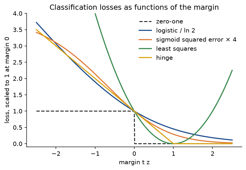
Logistic and hinge grow linearly for mistakes and vanish for confident correct answers. Least squares is the only one that punishes being too right, and the sigmoid squared error is the only bounded one, which flattens for confident mistakes.

The logistic loss is the binary cross-entropy rewritten with y = (1 + t)/2. The hinge is the loss of the support vector machine: its gradient is exactly zero once the margin reaches 1, so only points inside the margin or on the wrong side shape the solution, and it gives a decision but no probability. The logistic, hinge and least-squares losses are convex and classification-calibrated: with enough data and a flexible model, minimizing them recovers the Bayes decision rule. The multiclass hinge of Weston and Watkins is PyTorch's MultiMarginLoss:

Each wrong class whose score comes within the margin of the true score contributes, and the division by K is PyTorch's convention.

Contrastive and triplet losses

Some networks are trained to produce embeddings in which similar inputs lie close together, and their losses compare distances instead of targets. For a pair of embeddings at distance d, with s = 1 if the pair is similar and s = 0 otherwise, the contrastive loss with margin M is

Similar pairs are pulled together, dissimilar pairs pushed apart until they are at least M away and ignored after that. The triplet loss takes an anchor, a positive of the same identity and a negative of another, and asks only for the order of the two distances:

Most triplets soon satisfy the margin and contribute nothing, so training depends on mining hard or semi-hard negatives. The InfoNCE loss behind contrastive image-text training is a softmax cross-entropy in disguise. For a batch of B matching pairs with similarity logits S, divided by a temperature, row i is classified with label i, every other item of the batch serving as a negative (Multimodal models):

In code that is CrossEntropyLoss applied to the similarity matrix with labels 0 to B - 1.

How the loss shapes a decision boundary on noisy data

For a linear classifier with score z = wᵀx + b, the gradient of the average cost is an average over examples:

Each example pulls the boundary with force equal to the size of the derivative of its cost with respect to its score, and with leverage proportional to its distance from the origin, so what matters is how that force behaves for points far from the boundary:

• Cross-entropy: the force |σ(z) - y| tends to 1 for a confident mistake. A mislabelled point far on the wrong side pulls with full force and large leverage for as long as it stays wrong.
• Hinge: force 1 for every point with margin below 1, the same story.
• Least squares on ±1 targets: force |z - t|, growing with distance even for correctly classified points, which drag the boundary towards themselves.
• Sigmoid squared error: force |σ(z) - y| σ′(z), which tends to 0 for a confident mistake. Far mislabelled points are ignored once they are confidently misclassified. This is the learning slowdown again, now as a benefit; the price is a non-convex cost whose result depends on where training starts.

Convex losses cannot be robust to label noise in this sense: a convex function of the margin that decreases anywhere grows at least linearly as the margin goes to minus infinity, so the pull of a confident mistake never fades. Bounded losses can be. The section on noisy data under In practice measures the effect.

Worked example

Three small cases, each computed in double precision and shown to four decimals. Values written out from rounded terms can differ from the full-precision result in the last digit; where they do, the text says so.

One sigmoid neuron from two starting points

A neuron with one input x = 1.5, target y = 1, net input z = wx + b, output a = σ(z) and learning rate η = 0.25, trained with squared error, one half (a - y) squared, or with cross-entropy, -ln a, which is the binary cross-entropy for y = 1. Two starting points: a mild one, (w, b) = (-0.2, -0.2), and a saturated one, (w, b) = (-2.4, -1.4), whose output is confidently wrong.

Mild start. The net input is z = 1.5 × (-0.2) - 0.2 = -0.5, the output a = 1/(1 + e to the 0.5) = 0.3775 and σ′(z) = 0.3775 × 0.6225 = 0.2350.

• Squared error: cost (1/2) × 0.6225² = 0.1937; output error δ = -0.6225 × 0.2350 = -0.1463; weight gradient δx = -0.2194 and bias gradient -0.1463. One step gives w = -0.1451 and b = -0.1634, so z = -0.3811, a = 0.4059 and the cost falls from 0.1937 to 0.1765.
• Cross-entropy: cost -ln 0.3775 = 0.9741; output error δ = a - y = -0.6225; weight gradient -0.9337 and bias gradient -0.6225. One step gives w = 0.0334 and b = -0.0444, so z = 0.0057, a = 0.5014 and the cost falls from 0.9741 to 0.6903.

Saturated start. Now z = 1.5 × (-2.4) - 1.4 = -5, a = 1/(1 + e to the 5) = 6.6929 × 10⁻³ and σ′(z) = 6.6481 × 10⁻³. The small numbers are shown with four significant decimals in scientific notation, since four decimal places would round them away.

• Squared error: cost (1/2) × 0.9933² = 0.4933; output error δ = -0.9933 × 6.6481 × 10⁻³ = -6.6036 × 10⁻³; weight gradient -9.9053 × 10⁻³. One step gives w = -2.3975 and b = -1.3983, so z = -4.9946 and a = 6.7286 × 10⁻³, and the cost stays at 0.4933 to four decimals.
• Cross-entropy: cost -ln(6.6929 × 10⁻³) = 5.0067; output error δ = a - y = -0.9933; weight gradient -1.4900. One step gives w = -2.0275 and b = -1.1517, so z = -4.1929, a = 0.0149 and the cost falls from 5.0067 to 4.2079.

The two losses differ only in the factor σ′(z), so the ratio of their output errors is 1/σ′(z): 4.2553 at the mild start and 150.4199 at the saturated one. One step of cross-entropy moves the saturated neuron's net input by 0.8071; one step of squared error moves it by 0.0054.

Training both starts for 400 epochs turns this into the curves below:

• Mild start, squared error: the output first exceeds 0.5 at epoch 5 and 0.9 at epoch 92, and is 0.9055 after 100 epochs and 0.9571 after 400.
• Mild start, cross-entropy: epochs 1 and 13; 0.9874 after 100 epochs and 0.9969 after 400.
• Saturated start, squared error: epochs 206 and 293; 0.0141 after 100 epochs and 0.9367 after 400.
• Saturated start, cross-entropy: epochs 8 and 19; 0.9866 after 100 epochs and 0.9969 after 400.

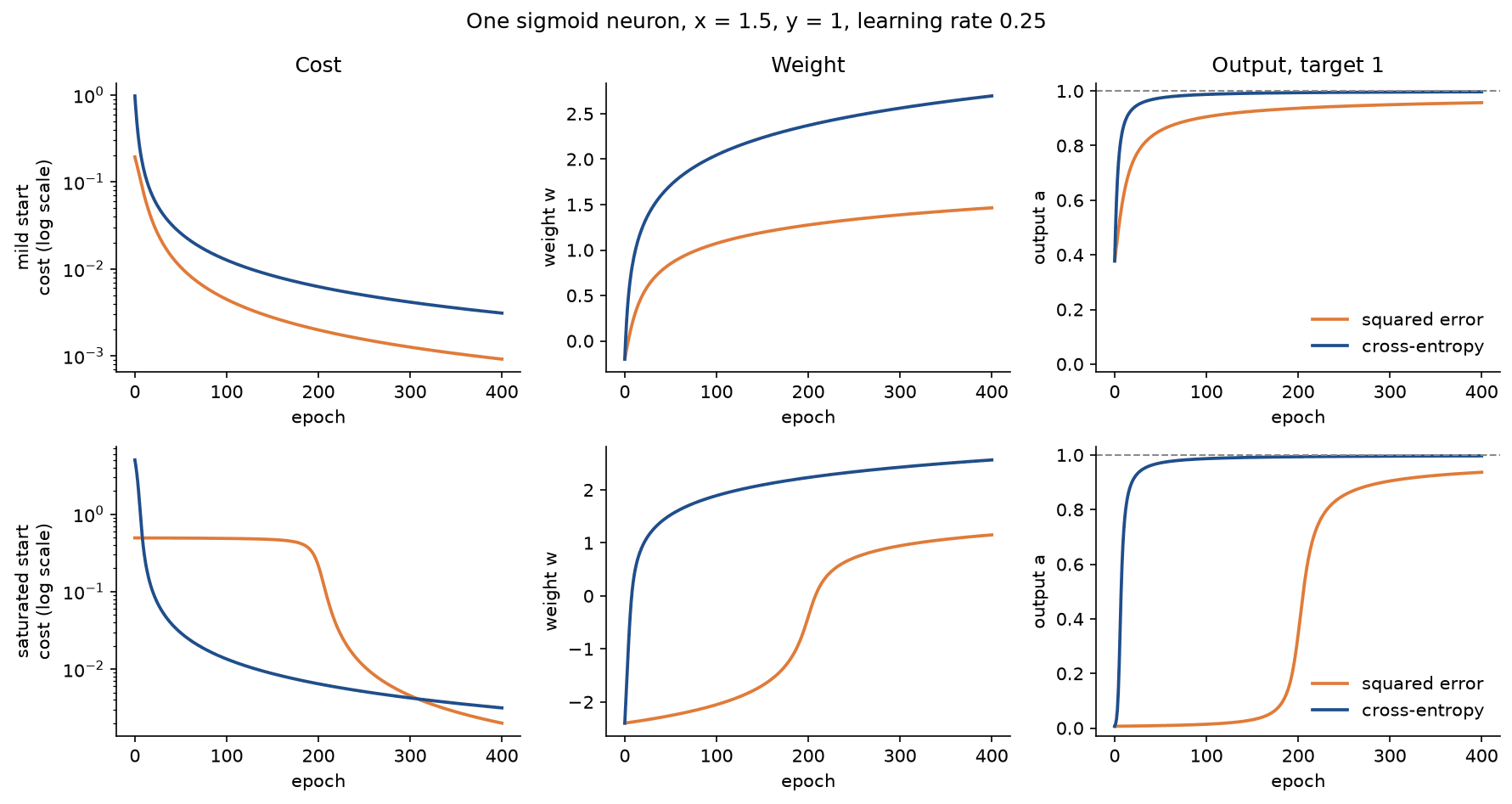
From the saturated start, squared error sits on a plateau for about two hundred epochs: the weight creeps up, the output stays near zero, and only once the output reaches the region where σ′ is large does it move quickly. Cross-entropy crosses a = 0.5 after 8 epochs, almost as fast as from the mild start.

Squared error is slower even from the mild start, because σ′(z) is at most 1/4 everywhere and shrinks again as the output approaches the target. The plot of the output error against the net input shows the cause in one picture: 1 - a for cross-entropy, largest when the neuron is most wrong, against (1 - a) a (1 - a) for squared error, which peaks at a = 1/3 with value 0.1481 and fades to zero at both ends.

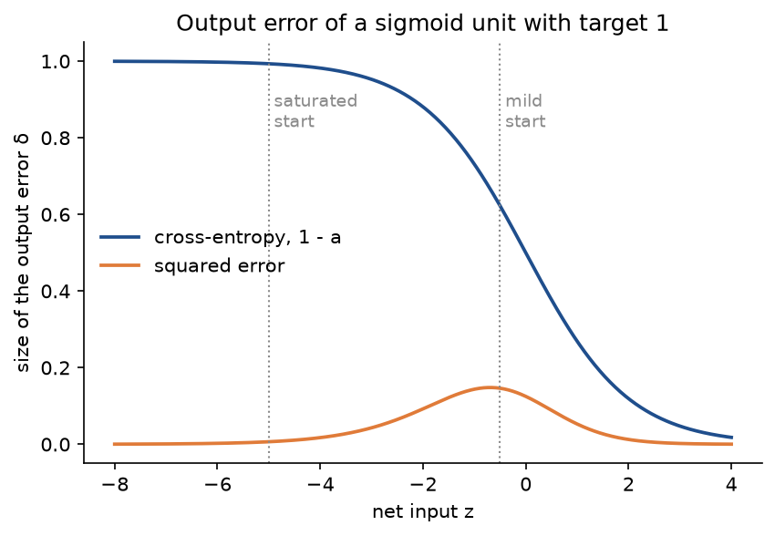
At the saturated start the cross-entropy error is close to its maximum of 1 while the squared-error one is almost zero, which is the whole learning slowdown in one vertical line.

One warning about the cost panels: after 400 epochs from the mild start, squared error reports a cost of 0.0009 and cross-entropy 0.0031, although the cross-entropy neuron is much closer to the target (output 0.9969 against 0.9571). Costs of different losses are on different scales and cannot be compared with each other; compare the predictions.

Softmax and log-likelihood for one example

Three classes with logits z = (2.0, 1.0, -0.5) and true class 2, so y = (0, 1, 0); in the code, classes are counted from zero and the label is 1.

• Log-sum-exp. The largest logit is M = 2. The shifted logits (0, -1, -2.5) have exponentials (1, 0.3679, 0.0821), whose sum is 1.4500 and its logarithm 0.3715, so LSE(z) = 2 + 0.3715 = 2.3715.
• Log-softmax, softmax and cost. The log-probabilities are z - LSE(z) = (-0.3715, -1.3715, -2.8715), the probabilities a = (0.6897, 0.2537, 0.0566), and the cross-entropy is minus the log-probability of the true class, LSE(z) - 1.0 = 1.3715.
• Output error. δ = a - y = (0.6897, -0.7463, 0.0566): the true logit should rise and the others fall, the first most because it holds most of the wrongly placed probability.

The same through the Jacobian. With J = diag(a) - a aᵀ, the rows of J are (0.2140, -0.1750, -0.0390), (-0.1750, 0.1893, -0.0144) and (-0.0390, -0.0144, 0.0534), and every row sums to zero. The gradient of the cost with respect to the outputs is (0, -1/a2, 0) = (0, -3.9414, 0). Only its second entry is nonzero, so Jᵀ times it is -3.9414 times the second row of J: (0.6897, -0.7463, 0.0566), exactly a - y. From the rounded entries the products are 0.6897, -0.7461 and 0.0568; the full-precision values agree with a - y to the last digit.

Label smoothing with ε = 0.1. The target becomes (1/30, 28/30, 1/30) = (0.0333, 0.9333, 0.0333) and the cost is 0.9 × 1.3715 + 0.1 × (0.3715 + 1.3715 + 2.8715)/3 = 1.2344 + 0.1538 = 1.3882, with output error a minus the smoothed target, (0.6563, -0.6796, 0.0233). At the optimum the true logit leads the others by ln 28 = 3.3322 and the cost equals the entropy of the target, 0.2911.

Gradient descent with step 1 on these three logits from zero shows the difference. Without smoothing the gap between the true logit and the first one is 5.6931 after 100 steps, 8.0049 after 1,000 and 10.3088 after 10,000, growing by about ln 10 per decade without limit; with smoothing it is 3.3321 after 100 steps and stays at 3.3322.

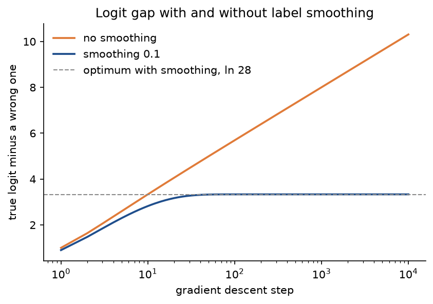
A straight line on a logarithmic step axis means the unsmoothed gap grows like the logarithm of the step count, forever; the smoothed one stops at its optimum.

Robust losses on five numbers

Five observations y = (2.0, 3.0, 3.5, 4.5, 12.0), the last one far from the rest, and a constant prediction ŷ = 4.0, so the residuals are r = y - ŷ = (-2, -1, -0.5, 0.5, 8). The Huber threshold is κ = 1 and the pinball level τ = 0.75. For each loss, the loss of each observation, then its pull, the derivative with respect to the prediction:

• Squared error: losses (2, 0.5, 0.125, 0.125, 32), mean 6.95; pulls (2, 1, 0.5, -0.5, -8), mean -1.
• Absolute error: losses (2, 1, 0.5, 0.5, 8), mean 2.4; pulls (1, 1, 1, -1, -1), mean 0.2.
• Huber: losses (1.5, 0.5, 0.125, 0.125, 7.5), mean 1.95; pulls (1, 1, 0.5, -0.5, -1), mean 0.2.
• Pinball: losses (0.5, 0.25, 0.125, 0.375, 6), mean 1.45; pulls (0.25, 0.25, 0.25, -0.75, -0.75), mean -0.15.

The outlier contributes 32 of the 34.75 total squared error and pulls with strength 8, enough to make the average pull negative, that is, to ask for a larger prediction, although four of the five observations are at most 4.5. Under the absolute and Huber losses its pull is 1 and the average pull is positive, asking for a smaller prediction: three observations lie below 4.0 and two above. The pinball loss with τ = 0.75 wants three quarters of the observations below the prediction; only three of five are, so it asks for a larger value.

The best constants make the same point. Squared error gives the mean, 5.0, a value no observation is near. Absolute error gives the median, 3.5. For the Huber loss, guess that the minimizer lies between 3.5 and 4.0; then the residuals of 2.0 and 12.0 are clipped to -1 and +1, and the condition reads -1 + (3 - ŷ) + (3.5 - ŷ) + (4.5 - ŷ) + 1 = 11 - 3ŷ = 0, so ŷ = 11/3 = 3.6667. The three middle residuals, -0.6667, -0.1667 and 0.8333, all lie inside [-1, 1], which confirms the guess. The pinball loss with τ = 0.25 gives 3.0 and with τ = 0.75 gives 4.5: with n = 5, n τ = 1.25 and 3.75 fall strictly between whole numbers, so each quantile is one of the observations.

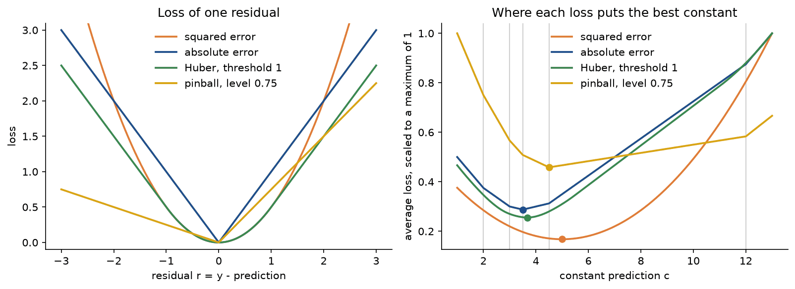
The left panel shows why the outlier matters to squared error alone: only the parabola keeps getting steeper. The right panel shows each average loss and the best constant it picks, with the five observations as thin vertical lines.

In PyTorch the same numbers come out as MSELoss 13.9 = 2 × 6.95, because it has no factor 1/2, L1Loss 2.4 and HuberLoss(delta=1.0) 1.95. Every number in this section is asserted by tests/test_worked.py and printed by the first three example scripts.

The code

The package loss_functions is plain NumPy, split into one module per idea. PyTorch, SciPy and scikit-learn are imported only inside the functions of comparisons.py and one function of pitfalls.py, so everything else works without them.

• arrays.py holds the Array type, as_array and reduce, which applies a "mean", "sum" or "none" reduction to per-entry losses.
• stable.py holds the overflow-free sigmoid, softplus and log-sigmoid, and log-sum-exp, log-softmax and softmax with the largest logit factored out.
• jacobian.py holds softmax_jacobian and output_delta, the transposed Jacobian times the gradient of the cost.
• targets.py holds one_hot, smooth_labels and entropy.
• regression.py holds the squared, absolute, Huber and pinball losses, each with its gradient with respect to the prediction, and the Gaussian and Laplace negative log-likelihoods.
• binary.py holds the binary cross-entropy on probabilities and on net inputs with an optional pos_weight, and the focal loss, with gradients with respect to the net input.
• categorical.py holds cross_entropy and cross_entropy_gradient with class-index or probability targets, class weights, label smoothing and PyTorch's reductions, and categorical_nll for the two-step form.
• margins.py holds the hinge with its gradient, the logistic margin loss, the multiclass hinge, and the contrastive and triplet losses.
• constants.py holds best_constant for the regression losses and huber_location, which solves the Huber condition by bisection.
• gradient_check.py holds central_difference, which the tests and the notebook use to check every hand-derived gradient.
• neuron.py holds neuron_step, which returns every quantity of one gradient step as a NeuronStep, train_neuron and first_epoch_above.
• worked.py holds the three worked examples as data and builders: first_steps, neuron_runs, trace_softmax, logit_gap_history, regression_pulls and sample_best_constants.
• linear.py holds a linear classifier trained by full-batch gradient descent under five losses.
• robust_fit.py holds fit_line, one gradient descent loop for a line under any regression loss, robust_fits and the measures line_gap, fraction_below and named_fit_loss.
• datasets.py generates the Gaussian classes, the noisy-label and imbalanced scenarios and the glitchy sensor readings from seeds.
• metrics.py holds accuracy, precision, recall and F1, the Brier score, and best_threshold, which picks a threshold on validation data.
• pitfalls.py holds small demonstrations of the mistakes under Pitfalls.
• cases.py builds random inputs for every loss and computes our values arranged by the name of the matching torch.nn class; comparisons.py computes the same with PyTorch, and the exact line fits with NumPy, SciPy and scikit-learn.
• plotting.py and experiment_plots.py draw every figure in the handbook's four colours and save it reproducibly.

Every loss returns one value per entry, or per example for cross_entropy with reduction="none", so reductions are explicit. The cross-entropy follows PyTorch's semantics exactly, including the less obvious ones: with class-index targets and class weights the mean divides by the sum of the weights of the examples, and label smoothing spreads ε uniformly over all K classes. Its gradient uses one formula for every case. Writing the cost of example i as minus the sum over k of a coefficient q times the log-probability, with coefficients that absorb the weights and the smoothing, the derivative with respect to logit j is a_j times the sum of the coefficients minus q_j, which is a - y whenever the coefficients sum to one:

coefficients, normalizer = cross_entropy_coefficients(logits, targets, weight, label_smoothing)
gradient = softmax(logits) * np.sum(coefficients, axis=1, keepdims=True) - coefficients
if reduction == "mean":
    return gradient / normalizer

The stable log-softmax subtracts the largest logit once and never forms a probability:

def log_softmax(z: ArrayLike, axis: int = -1) -> Array:
    shifted, _ = shifted_by_max(z, axis)
    return shifted - np.log(np.sum(np.exp(shifted), axis=axis, keepdims=True))

The examples and the project import the package, so install the repository first as described in the main README. Each example demonstrates one idea and runs in a few seconds from the repository root:

• examples/learning_slowdown.py prints the first step of the neuron from both starts and a summary of 400 epochs, and saves the learning-slowdown and output-error figures.
• examples/softmax_by_hand.py prints the softmax example through log-sum-exp and through the Jacobian, repeats it with label smoothing, and saves the logit-gap figure.
• examples/five_observations.py prints the loss and pull of each observation under the four regression losses and the best constants, and saves the regression-losses figure.
• examples/noisy_labels.py compares the margin losses and trains a linear classifier under four of them on noisy labels, saving the margin-losses and decision-boundaries figures.
• examples/common_mistakes.py demonstrates each pitfall below with numbers.
• examples/compare_with_libraries.py checks every loss and six gradients against torch.nn and autograd, and the gradient-descent lines of the project against exact solvers.

python neural-networks/loss-functions/examples/learning_slowdown.py
python neural-networks/loss-functions/examples/softmax_by_hand.py
python neural-networks/loss-functions/examples/five_observations.py
python neural-networks/loss-functions/examples/noisy_labels.py
python neural-networks/loss-functions/examples/common_mistakes.py
python neural-networks/loss-functions/examples/compare_with_libraries.py

The sample project, project/outliers_and_imbalance.py, applies the topic to two kinds of messy data where the default loss misleads. The first part simulates 400 readings of a sensor at inputs spread evenly over [0, 10]. The true relation is 1 + 0.5x, the Gaussian noise grows from a standard deviation of 0.3 at x = 0 to 1.5 at x = 10, and 24 readings, 6 %, carry a glitch that adds between 8 and 16. The project fits a single linear unit, the output layer of any regression network, under squared error, absolute error, the Huber loss with κ = 1 and the pinball loss at levels 0.1 and 0.9. Every fit uses the same gradient descent loop, in which only the gradient of the loss changes. The input is standardized, and the step shrinks over time:

The shrinking step matters for the absolute and pinball losses, whose gradients keep their full size right up to the minimum: with a fixed step the line would bounce around the minimum forever. With the defaults, 20,000 steps and T = 50, the fits are:

• Squared error: slope 0.4445, intercept 2.0020, on average 0.7247 away from the true line over [0, 10].
• Absolute error: slope 0.5135, intercept 1.0266, 0.0942 away.
• Huber: slope 0.5087, intercept 1.0675, 0.1108 away.
• 0.1-quantile: slope 0.3338, intercept 0.6937, 0.0331 away from the 0.1-quantile line of clean readings.
• 0.9-quantile: slope 0.6105, intercept 1.8905, 0.2895 away from the 0.9-quantile line of clean readings.

On 4,000 fresh readings drawn the same way, glitches included, 10.37 % fall below the 0.1-quantile line and 89.92 % below the 0.9-quantile line, so the two lines bracket 79.55 % of new readings, as an 80 % interval should. The project then scales every glitch from zero to twice its size, keeping everything else fixed, and refits. The squared-error fit moves away from the true line in proportion to the glitches, from 0.0087 to 1.4558. The absolute, Huber and 0.9-quantile fits stop moving at 0.0942, 0.1108 and 0.2895 as soon as the glitched readings lie clearly above them, because from then on those readings pull with a fixed force however far away they are.

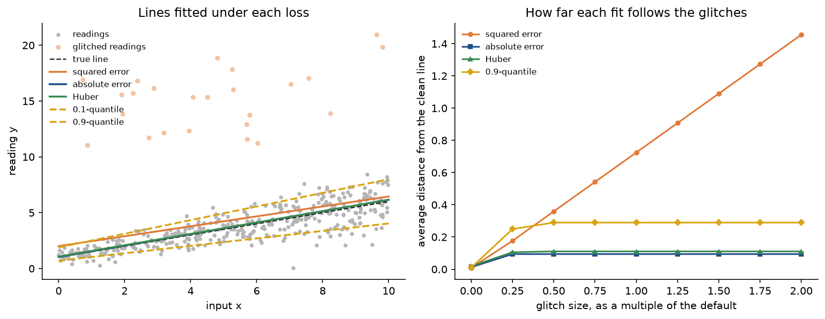
The left panel shows the fits on the default data; the quantile lines fan out because the noise grows with x. The right panel is the robustness of each loss in one picture: only squared error keeps following the glitches as they grow. The 0.9-quantile line does move at first, to 0.2895, because 6 % of glitched readings change which readings form the top tenth; a pinball line is robust to how far outliers are, not to how many there are.

The second part trains a linear classifier on 1,000 examples of two overlapping Gaussian classes with 5 % positives and tests it on 10,000 examples with the same rate. Plain cross-entropy at the default threshold of 0.5 has accuracy 0.9620, precision 0.6935, recall 0.4300 and F1 0.5309, and its mean predicted probability, 0.0532, is close to the true rate of 0.05; its Brier score is 0.0289. With pos_weight 19, the ratio of negatives to positives, recall rises to 0.8800 at precision 0.2536 (F1 0.3937), the mean probability inflates to 0.2244 and the Brier score to 0.1002. Focal loss with γ = 2 leaves the decisions almost unchanged (precision 0.6845, recall 0.4340, F1 0.5312) and inflates the probabilities to a mean of 0.1579, Brier score 0.0448. Moving the plain model's threshold instead does what the weight did without retraining. At 1/(1 + 19) = 0.05 it gives precision 0.2593 and recall 0.8800, and the same decision as the weighted model on 99.62 % of test points. At 0.35, the threshold with the best F1 on a separate validation set of 2,000 examples, it gives precision 0.6152, recall 0.5660 and F1 0.5896, the best F1 of all the models.

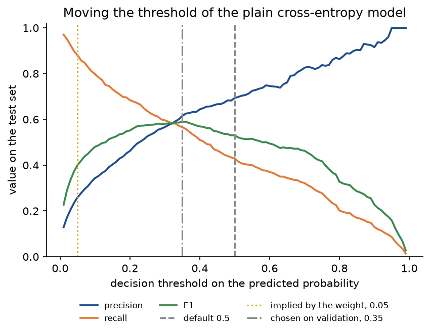
Every model in the comparison is a point on these curves or close to one: the class weight picks the point at 0.05, the default picks 0.5, and the validation set picks the point that balances the two kinds of error for F1. Choosing the point explicitly keeps the probabilities calibrated.

Options such as --seed, --samples, --outlier-fraction, --delta, --quantiles, --steps, --classifier-steps and --gamma change the setup, and --figures sends the two PNGs to another folder so a custom run does not overwrite the ones shown here. The default run takes about ten seconds on one CPU thread.

python neural-networks/loss-functions/project/outliers_and_imbalance.py
python neural-networks/loss-functions/project/outliers_and_imbalance.py --outlier-fraction 0.15

The notebook loss_functions.ipynb follows the order of this page: the noise models checked numerically, the one-neuron experiment, softmax and its Jacobian with a finite-difference check, stable log-sum-exp in double and single precision, label smoothing, the robust, margin and embedding losses, the decision-boundary experiment, the project's two experiments in brief, each pitfall, and the comparison with torch.nn. The tests in tests check the worked examples value by value, every gradient against finite differences, the experiments quoted under In practice and the agreement with PyTorch, SciPy and scikit-learn, and run in about ten seconds:

python -m pytest neural-networks/loss-functions

Every dataset is synthetic, generated by datasets.py from fixed seeds, so nothing is downloaded and no licence is involved.

In practice

Agreement with the libraries

PyTorch's losses take the net input wherever the stable form needs it, average over every entry by default, and have conventions of their own. In double precision, on three random cases, our implementation agrees with every one of the sixteen loss configurations below to within 4.4 × 10⁻¹⁶, a few units in the last place, and the six gradients compared agree with autograd to within 1.1 × 10⁻¹⁶ (examples/compare_with_libraries.py, tests/test_comparisons.py). What each class expects:

• MSELoss is the mean of twice our squared_error: it has no factor one half and averages over every entry.
• L1Loss is the mean of absolute_error; its gradient is the sign of a - y, and 0 at a tie.
• HuberLoss(delta) is the mean of huber, and SmoothL1Loss(beta) is that divided by β, so the two agree only for β = 1.
• GaussianNLLLoss takes the variance and drops the constant one half of ln 2π unless full=True, matching gaussian_nll.
• BCELoss takes probabilities and clamps the logarithm at -100; BCEWithLogitsLoss(pos_weight) takes the net input, and its mean divides by the number of entries, not by the weights.
• CrossEntropyLoss takes logits with class indices or probabilities. With label_smoothing the uniform part includes the true class; with weight the mean divides by the summed weights of the batch's labels.
• NLLLoss after LogSoftmax is the two-step form of CrossEntropyLoss, our categorical_nll of the softmax.
• MultiMarginLoss divides the multiclass hinge by the number of classes, and TripletMarginLoss adds a small eps to the difference before the norm, which triplet_loss(..., eps=1e-6) reproduces.

The focal loss has no torch.nn class; torchvision.ops.sigmoid_focal_loss computes the same formula as focal_loss, but torchvision is not in any dependency group here, so that agreement is not tested. The pinball loss is sklearn.metrics.mean_pinball_loss and loss="quantile" in scikit-learn's gradient boosting models. The project's lines can be checked against solvers that know nothing of gradient descent: least squares in closed form, BFGS from SciPy on the average Huber loss, and the linear program of scikit-learn's QuantileRegressor without a penalty for the absolute and pinball lines. On the project's default data, the gradient-descent lines reach the exact minimum to within 3 × 10⁻⁷ in average loss. The squared-error and Huber lines agree to the printed digits, and the absolute and pinball lines differ by at most 4 × 10⁻⁴ in an intercept, because the minimum of a piecewise linear loss can be nearly flat.

Choosing a loss

The tree turns the derivations above into a first choice: decide what the target is and what the noise looks like, and the output layer and the loss follow. The green boxes name the output layer and the PyTorch class for each; every regression box uses an identity output.

The decision boundary on noisy data

Two Gaussian classes in the plane, 100 points each with standard deviation 0.9 around (-1, -0.5) and (1, 0.5), a linear classifier trained by full-batch gradient descent from zero for 5,000 steps, and a clean test set of 4,000 points (examples/noisy_labels.py). Then 20 points are added far on the side of class 1, around (6, 5) and labelled 1, or around (4, 3) and labelled 0. Accuracy on the clean test set:

• Clean training data: cross-entropy 0.8958, sigmoid with squared error 0.8950, least squares 0.8955, hinge 0.8948.
• With the 20 far points correctly labelled: cross-entropy 0.8958, sigmoid with squared error 0.8950, least squares 0.8415, hinge 0.8948.
• With the 20 far points mislabelled: cross-entropy 0.7462, sigmoid with squared error 0.8950, least squares 0.7462, hinge 0.8565.

On clean data the four losses are within a tenth of a percentage point of each other. Correctly labelled far points move only least squares, which penalizes them for being too far on the right side and tilts its boundary to bring them closer. Mislabelled far points drag the cross-entropy and least-squares boundaries through the middle of class 1 and cost them 15 points of accuracy. The hinge suffers less, since its pull per point is 1 and the far points have to compete with every point inside the margin. The bounded sigmoid squared error ignores them completely: they become confidently misclassified early in training, their gradient vanishes, and the boundary is the clean one.

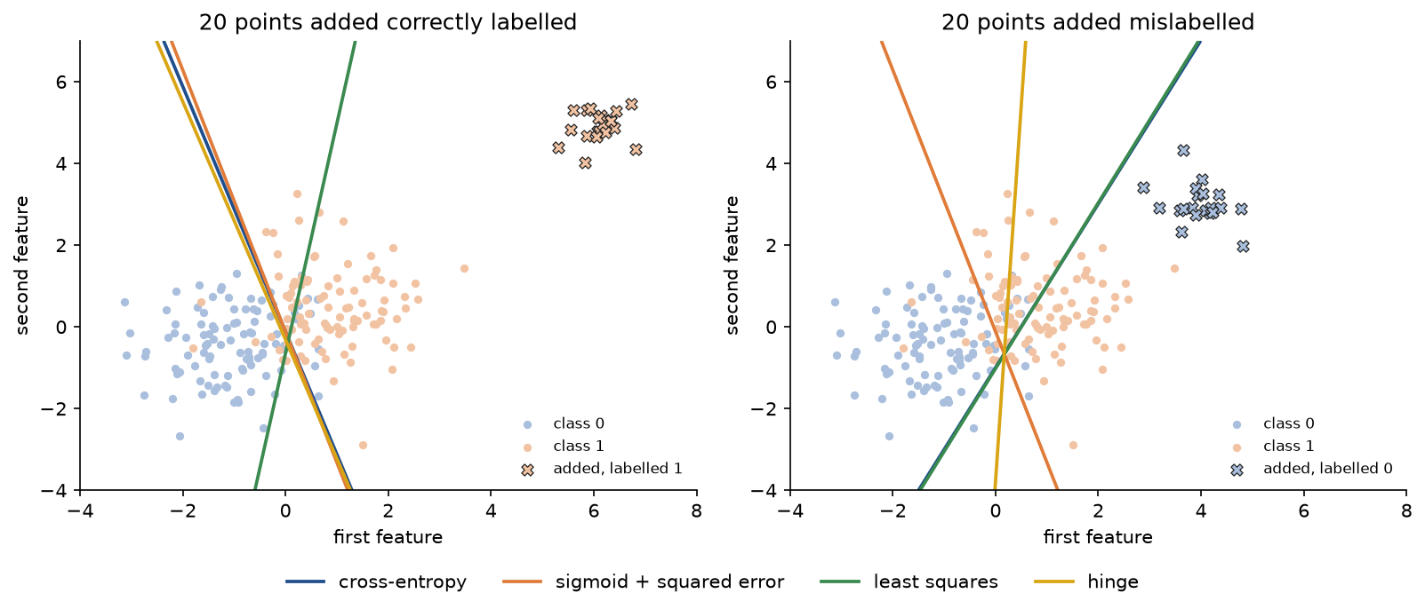
The lesson is not that sigmoid squared error is a good default. It is non-convex, it learns slowly from the same saturation, and it ignores a confidently misclassified point whether that point is mislabelled or merely hard. When gross label errors are suspected, the usual remedies are to find and fix them, to use a bounded or truncated loss, or to model the noise explicitly.

When to use which:

• Use the loss whose noise model fits the targets, paired with its matching output: identity with squared error, sigmoid with binary cross-entropy, softmax with categorical cross-entropy. In PyTorch that means no activation at the end of the model and the logits passed to BCEWithLogitsLoss or CrossEntropyLoss.
• For imbalanced classes, train with plain cross-entropy and choose the threshold on validation data for the precision and recall you need, as the project does. Class weights do the same job less transparently; they are convenient when the threshold cannot be changed after training.
• Reach for focal loss when easy examples vastly outnumber the informative ones, as in dense detection, and recalibrate its outputs if they are read as probabilities.
• Use label smoothing for large classifiers that overfit or are overconfident, not for a model that will serve as a teacher.
• Use the Huber loss when a few targets are much farther off than the rest, with the threshold set from the noise level, and the pinball loss when the question is about a quantile or an interval.
• Use the from-scratch losses here to learn the conventions and to test your own; in training code, use the library classes, which are fused, stable and run on accelerators.

Pitfalls

• Squared error on a sigmoid output. The output error carries σ′(z) and vanishes for a confidently wrong neuron: in the worked example it is 150 times smaller than under cross-entropy and costs two hundred epochs on a plateau (examples/learning_slowdown.py). The same holds for a softmax output with squared error.
• Expecting cross-entropy to cure every vanishing gradient. It cancels σ′ at the output layer only. A hidden sigmoid unit with net input -5 still multiplies the error passing through it by σ′(-5) = 0.0066 in B2, whatever the loss.
• Applying the activation twice. CrossEntropyLoss applies log-softmax and BCEWithLogitsLoss applies the sigmoid. A model that already ends in softmax and feeds probabilities to CrossEntropyLoss can never reach zero loss: even a perfect one-hot prediction costs ln(1 + (K - 1)/e), 1.4612 for ten classes. The gradient is squeezed too: for the worked example's logits it becomes (0.4592, -0.7030, 0.2438) instead of (0.6897, -0.7463, 0.0566) (examples/common_mistakes.py, and the diagram under How it works). Some frameworks expose the choice as a from_logits flag that must match what the model outputs.
• Sigmoid followed by BCELoss. In double precision σ(40) rounds to exactly 1. BCELoss then clamps ln 0 to -100 and reports a loss of 100 with a gradient of exactly zero, while BCEWithLogitsLoss on the net input reports 40 with gradient 1 (examples/common_mistakes.py). Clipping probabilities by hand hides the same problem and also zeroes the gradient.
• Computing the softmax or its logarithm naively. exp(z) / exp(z).sum() returns nan for logits around ±1000, and in single precision log(softmax(z)) is minus infinity as soon as a logit trails the largest by more than about 104: for z = (0, -120) it gives minus infinity where the correct value is -120 (examples/common_mistakes.py). Use log_softmax, logsumexp and the loss functions that take logits.
• Comparing loss values across losses or settings. After 400 epochs from the mild start the squared-error neuron reports a cost of 0.0009 and the cross-entropy neuron 0.0031, though the second is much closer to the target. Label smoothing raises the floor of the loss from 0 to the entropy of the smoothed target, 0.2911 in the worked example, so smoothed and unsmoothed losses cannot be compared either. Compare models on a metric of the predictions.
• Forgetting what the mean divides by. MSELoss averages over every entry and has no factor 1/2, so for one output its gradient is twice that of one half (a - y) squared. CrossEntropyLoss with class weights divides by the sum of the weights of the batch's labels, not by the batch size. With weights 1 and 4 on the labels (0, 1, 1) of a three-example batch, the weighted mean is 0.3993, and dividing by 3 would give 1.1979 (examples/common_mistakes.py). An example's contribution therefore depends on the rest of its batch. With probability targets, by contrast, the mean divides by the batch size.
• Shapes that broadcast. Predictions of shape (m, 1) minus targets of shape (m,) form an m × m matrix. For predictions (0.5, 1.0, 2.5, 2.0) and targets (0, 1, 2, 3) the intended mean squared error is 0.375 and the broadcast value 1.875; PyTorch warns, NumPy does not (examples/common_mistakes.py). CrossEntropyLoss also needs integer class indices of type int64, or floating-point probabilities of the same shape as the logits, never one-hot vectors cast to integers.
• Treating class weights as a fix for imbalance. A weight w adds ln w to the logits and is equivalent to moving the threshold to 1/(1 + w); the probabilities of the weighted model are no longer calibrated. In the project the weighted model's mean probability is 0.2244 for a true rate of 0.05, and it agrees with the plain model at threshold 0.05 on 99.62 % of test points. Resampling the rare class has the same effect. Decide the threshold from the costs of the two kinds of error, on validation data.
• Reading focal-loss outputs as probabilities. Its minimizer is pulled towards 1/2: in the project the mean predicted probability is 0.1579 for a true rate of 0.05.
• Confusing HuberLoss and SmoothL1Loss. SmoothL1Loss(beta) is HuberLoss(delta=beta) divided by β. For predictions (0, 0.5, 3) and targets (1, -1.5, 0.2), β = 0.5 gives 0.8417 and 1.6833, and β = 2 gives 2.0333 and 1.0167 (examples/common_mistakes.py). The Huber threshold is in units of the target, so a value tuned on standardized targets is wrong for raw ones.
• The sign of the pinball residual. The loss is defined on r = y - ŷ. Written on ŷ - y it fits the (1 - τ)-quantile: asked for the 0.75-quantile of the five observations, the swapped loss returns 3.0, the 0.25-quantile, instead of 4.5 (examples/common_mistakes.py). Quantile models fitted separately for several levels can also cross; check that the predicted quantiles are ordered.
• A fixed step for a non-smooth loss. The absolute and pinball gradients do not shrink near the minimum, so gradient descent with a constant step keeps jumping across it. fit_line shrinks the step like one over the square root of the step count, which is why the project's lines reach the exact minimum.
• Using a softmax when labels are not exclusive. A softmax forces the outputs to compete, so an image that shows both a cat and a dog can never get high probability for both. Use one sigmoid per label with binary cross-entropy for multi-label targets.
• Claiming a bounded loss is always more robust. It ignores any confidently misclassified point, mislabelled or merely hard, and its cost is non-convex, so the result depends on the starting point; the notebook's Try it section suggests starting it from the cross-entropy solution.

Further reading

• M. A. Nielsen, Neural Networks and Deep Learning, chapter 3, 2015. A free online book with the cross-entropy cost, the learning slowdown and softmax for a sigmoid network.
• I. Goodfellow, Y. Bengio and A. Courville, Deep Learning, MIT Press, 2016, sections 5.5 and 6.2. Maximum likelihood and the choice of cost function and output unit.
• C. M. Bishop, Pattern Recognition and Machine Learning, Springer, 2006, sections 4.3 and 5.2. Canonical links and the matching of output activations and error functions.
• P. McCullagh and J. A. Nelder, Generalized Linear Models, second edition, Chapman and Hall, 1989. The exponential family and canonical links in general.
• T. Gneiting and A. E. Raftery, "Strictly proper scoring rules, prediction, and estimation", Journal of the American Statistical Association 102(477), 359-378, 2007.
• P. J. Huber, "Robust estimation of a location parameter", Annals of Mathematical Statistics 35(1), 73-101, 1964.
• R. Koenker and G. Bassett, "Regression quantiles", Econometrica 46(1), 33-50, 1978.
• P. L. Bartlett, M. I. Jordan and J. D. McAuliffe, "Convexity, classification, and risk bounds", Journal of the American Statistical Association 101(473), 138-156, 2006. When surrogate losses recover the Bayes classifier.
• P. M. Long and R. A. Servedio, "Random classification noise defeats all convex potential boosters", Machine Learning 78(3), 287-304, 2010.
• C. Elkan, "The foundations of cost-sensitive learning", Proceedings of the 17th International Joint Conference on Artificial Intelligence, 2001. Class weights, resampling and the moved threshold.
• C. Szegedy, V. Vanhoucke, S. Ioffe, J. Shlens and Z. Wojna, "Rethinking the Inception architecture for computer vision", CVPR 2016. Introduces label smoothing.
• R. Müller, S. Kornblith and G. E. Hinton, "When does label smoothing help?", NeurIPS 2019.
• T.-Y. Lin, P. Goyal, R. Girshick, K. He and P. Dollár, "Focal loss for dense object detection", ICCV 2017.
• R. Hadsell, S. Chopra and Y. LeCun, "Dimensionality reduction by learning an invariant mapping", CVPR 2006. The contrastive loss.
• F. Schroff, D. Kalenichenko and J. Philbin, "FaceNet: a unified embedding for face recognition and clustering", CVPR 2015. The triplet loss with online mining.
• A. van den Oord, Y. Li and O. Vinyals, "Representation learning with contrastive predictive coding", arXiv:1807.03748, 2018. The InfoNCE loss.