Support vector machines

When two classes can be separated by a straight line, infinitely many lines do it, and a perceptron or an unregularized logistic regression stops at whichever one it happens to reach. A support vector machine picks the line that stays as far as possible from the nearest points of both classes. That choice has three consequences that make the method worth knowing in detail: the solution is the unique optimum of a convex problem, it depends only on the few training points that touch the margin, and because the training points enter only through inner products, replacing those inner products by a kernel turns the same algorithm into a nonlinear classifier at no extra conceptual cost. This page derives the margin and the hard-margin problem, its Lagrange dual and KKT conditions, the soft margin and its hinge-loss form, two training algorithms (Pegasos on the primal and SMO on the dual), kernels and Mercer's condition, multiclass schemes, scaling and Platt scaling. An eight-point problem is solved by hand, everything is implemented from scratch in NumPy, and every solver is checked against scikit-learn's SVC and LinearSVC. Afterwards you will be able to solve a small SVM on paper, write a working SMO, choose C and γ deliberately and recognize the mistakes that make SVMs look worse than they are. It builds on Logistic regression and on the Lagrangians of Calculus and optimization.

To run the code in this topic, install the base and ml groups.

Intuition

Picture the two classes as two groups of points and the classifier as a road between them. Among all straight roads that keep each group on its own side, choose the widest one. The centre line of that road is the decision boundary, and the road's edges touch a few points of each class. Those points are the support vectors: they hold the road in place, and every other point could move around freely, as long as it stays off the road, without changing anything.

Why the widest road? A boundary that passes close to training points will misclassify new points that differ only slightly from them, while a wide road tolerates such perturbations. The width is also a measure of capacity that does not depend on the number of features, which is why maximum-margin classifiers generalize well even in very high dimensions.

Real data rarely allow a clean road. The soft margin lets some points stand on the road or even on the wrong side, at a price C per unit of intrusion, and trades the road's width against the total intrusion. Small C buys a wide road with many intruders, large C a narrow road with few.

Curved boundaries come from the kernel trick. Map every point into a richer space, for example by adding the squares and the product of its two coordinates as extra coordinates, and build the straight road there; seen in the original plane, the road is curved. The training problem only ever needs inner products of mapped points, and for many useful maps these can be computed directly from the original points, even when the mapped space has infinitely many dimensions.

The map shows how the sections below depend on each other. The two green boxes are the training algorithms: Pegasos works on the primal problem written with the hinge loss, SMO on the dual, and only the dual route admits kernels.

How it works

Notation

The training set has n examples. Example i has an input x, a column vector of d features, and a label y that is -1 or +1. The classifier is the hyperplane with normal vector w and offset b. Each example also gets a Lagrange multiplier α, its dual variable, and in the soft margin a slack ξ. C > 0 is the price of one unit of slack, λ = 1 / (nC) is the same price written as a regularization strength, φ is a feature map and K the kernel it induces, and γ is the width parameter of the RBF and polynomial kernels (not a margin). The set S holds the support vectors, the examples with α > 0.

The formula images carry the example index as a subscript. In the text, a single point is named by its index, so x4, y4 and α4 are the input, label and multiplier of point 4, and Kij is the kernel value of points i and j.

The separating hyperplane and the geometric margin

The decision value of a point is a linear function, and its sign is the predicted class:

The points with f(x) = 0 form a hyperplane with normal vector w. To find the distance of a point x from it, write x as the foot h of its perpendicular on the hyperplane plus r steps along the unit normal, where r is the signed distance, positive on the side w points to. Applying f and using f(h) = 0:

Multiplying by the label gives the geometric margin of example i, its distance from the hyperplane with a plus sign when it lies on its own side:

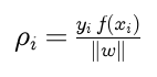
A classifier separates the data when every geometric margin is positive, and the margin of the data set is the smallest of them. The product y f(x) without the division is the functional margin. The pair (w, b) is not unique: multiplying both by any c > 0 describes the same hyperplane and the same classifier. Functional margins scale with c, geometric margins do not. The scale is fixed by the canonical normalization, which makes the nearest points have functional margin exactly one and geometric margin 1 / ‖w‖:

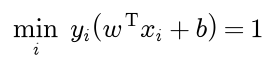
From here on every hyperplane is written in this scaling, so the points nearest to it have y f(x) = 1 exactly and every other point has y f(x) > 1.

The margin width, derived with consistent signs

Under the canonical normalization the nearest points lie on the two margin hyperplanes f = +1 and f = -1. Take any point x₊ on the first and any point x₋ on the second:

Subtracting equation 2 from equation 1 removes b. The width of the margin is the length of the component of x₊ - x₋ along the unit normal:

Three details keep the signs straight:

• The difference is taken from the negative margin to the positive one, x₊ - x₋, which is the direction w points in, so the projection is positive.
• Each point is substituted into its own equation, so the dot product of w with x₊ is 1 - b and with x₋ it is -1 - b. Exchanging them halfway through, or projecting x₋ - x₊, yields -2 / ‖w‖.
• The two points need not face each other. Any pair on the two hyperplanes gives the same projection, because moving either point within its hyperplane moves it perpendicular to w.

The same result follows from the distance formula: each margin hyperplane lies at distance 1 / ‖w‖ from the boundary, on opposite sides.

The hard-margin primal problem

Maximizing the width 2 / ‖w‖ subject to every point being on the correct side of its margin hyperplane is the same as minimizing ‖w‖, or the smooth and convex ‖w‖² / 2:

The constraints are affine and the objective is a strictly convex quadratic in w, so this is a convex quadratic program. It has a solution exactly when the classes are linearly separable, w is unique, and at the optimum both classes have at least one point on their margin, which fixes b. Writing one constraint y (wᵀx + b) ≥ 1 instead of separate inequalities for each class uses the labels -1 and +1: for y = -1 it reads wᵀx + b ≤ -1.

Lagrange duality and the KKT conditions

The general theory, Lagrangians, the KKT conditions and why they are sufficient for convex problems, is in Calculus and optimization. Written as a quantity that must not exceed zero, constraint i is 1 - y (wᵀx + b) ≤ 0, and with one multiplier α ≥ 0 per constraint the Lagrangian is

Setting its derivatives with respect to w and b to zero gives the two stationarity conditions, and together with feasibility and complementary slackness they form the KKT conditions:

Because the objective is convex and the constraints are affine, these conditions are both necessary and sufficient: any (w, b, α) that satisfies all five is optimal. This is what makes a hand solution possible. Guess which constraints are active, solve the resulting linear equations, and accept the guess if the solution is feasible with nonnegative multipliers.

The dual problem

The dual function is the minimum of the Lagrangian over w and b. The Lagrangian is linear in b with coefficient minus the sum of αy, so the minimum over b is minus infinity unless that sum is zero. Under that condition the minimum over w of the convex quadratic is at w = Σ α y x, and substituting it gives

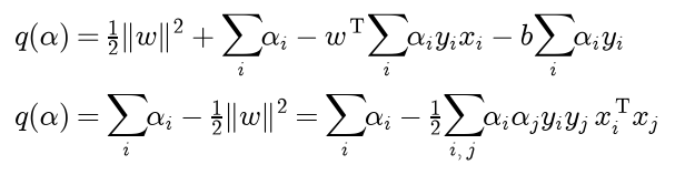
The dual problem maximizes this over the feasible multipliers:

Q is positive semidefinite, so the dual is a concave maximization, and for this problem strong duality holds: the dual optimum equals the primal optimum ‖w‖² / 2. Two useful identities follow at the optimum. Summing complementary slackness over i shows that the sum of α y f(x) equals the sum of α, and the left side is wᵀ Σ α y x + b Σ α y = ‖w‖², so

The offset comes from any support vector s, because y f(x) = 1 there and 1 / y = y:

Implementations average this over the support vectors to reduce rounding error.

Why only the support vectors matter

Complementary slackness forces α = 0 for every point strictly outside the margin, where y f(x) > 1. Such points drop out of w = Σ α y x and out of the decision function, which becomes a sum over the support vectors alone:

Delete every point with α = 0 and train again: the old solution still satisfies all KKT conditions of the smaller problem, so it is still optimal. Two practical facts follow. Prediction costs one inner product per support vector, not per training point. And in leave-one-out cross-validation, leaving out a point with α = 0 cannot change the classifier, so only support vectors can be misclassified when held out: the leave-one-out error is at most the number of support vectors divided by n.

The soft margin

When the classes overlap, no (w, b) satisfies every constraint. The soft margin gives each example a slack ξ ≥ 0, relaxes its constraint to y f(x) ≥ 1 - ξ and charges C per unit of slack:

A slack between 0 and 1 puts the point inside the margin but on the correct side; a slack above 1 puts it on the wrong side, so the total slack bounds the number of training errors. The Lagrangian gets a second set of multipliers μ ≥ 0 for the constraints ξ ≥ 0, and stationarity in ξ caps every α at C:

The slacks and the μ disappear from the dual, which is the hard-margin dual with a box:

Complementary slackness for both sets of multipliers sorts the examples into three groups:

Points with α = 0 are on or outside the margin and have no influence. Points with α strictly inside the box lie exactly on the margin, and the offset is computed from them. Points at the bound C lie inside the margin, or on the wrong side when y f(x) < 0. As C grows the box disappears and, for separable data, the hard margin returns.

The hinge-loss form

For a fixed hyperplane the cheapest slack that satisfies both constraints on ξ is max(0, 1 - y f(x)). Substituting it removes the constraints:

The function of the functional margin m = y f(x) inside the sum is the hinge loss. Dividing the objective by nC does not move its minimizer and gives the regularized-risk form:

This is the same template as L2-regularized logistic regression, with a different loss of the margin:

The hinge loss is convex, bounds the 0-1 loss from above, and is exactly zero for m ≥ 1. The logistic loss is never zero, so every training point keeps some influence on a logistic model, while a support vector machine ignores the points beyond its margin.

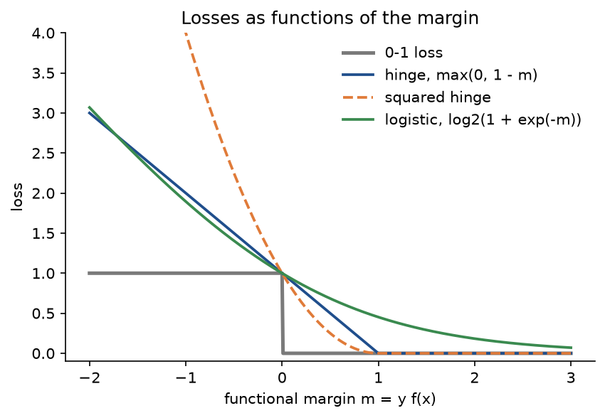
The plot draws the logistic loss divided by ln 2 so that all curves pass through 1 at m = 0. The squared hinge, the default of LinearSVC, punishes large violations much harder than the hinge, which makes it smoother but more sensitive to outliers.

Training the primal: Pegasos

The hinge loss has a kink at m = 1, so F has no gradient there, but it has a subgradient: -y x for an example with margin below one and 0 otherwise. Pegasos is stochastic subgradient descent on F with a step size matched to its strong convexity. At step t it draws a mini-batch of k examples, collects those with margin below one in a set A, and updates

optionally followed by a projection onto the ball of radius 1 / √λ, which contains the optimum. For a λ-strongly convex objective this step size gives an expected suboptimality of order log T / (λT) after T steps; averaging the iterates of the second half of the run removes the logarithm. The cost per step does not depend on n, which is the method's appeal for large data sets, and small λ, that is large C, is its weakness.

Pegasos as stated has no offset. The usual remedy, also used by LinearSVC, appends a constant feature of value s to every input, so that b is s times the weight of that feature. The offset is then regularized too, with weight 1 / s², which is a slightly different problem from the one above; a larger s weakens the penalty.

Training the dual: SMO

Write the soft-margin dual as a minimization of D over the box and the balance condition, with any kernel in Q. Changing one multiplier alone would break the balance condition, so sequential minimal optimization changes two at a time: moving αi by +yi t and αj by -yj t keeps Σ α y fixed. SMO tracks a score g for every example, the gradient of the dual in the direction its multiplier is allowed to move:

Along the move the dual is a parabola in t, because the labels square to one:

The best unconstrained step is the gap divided by the curvature κ. The box limits how far each multiplier may travel: the room r of a multiplier is C - α if it moves up and α if it moves down. The step is the smallest of the three:

Afterwards every score changes by t times the difference of two kernel columns, which is all the work a step needs. Which pair? Translate the three groups of the soft margin into conditions on g. A point with y = +1 and α = 0 needs u + b ≥ 1, that is b ≥ g; with α = C it needs b ≤ g; for y = -1 the inequalities reverse. Collecting them into two sets:

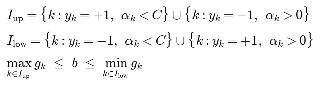
SMO picks i as the point of I up with the largest score and j as the point of I low with the smallest, the maximal violating pair, and stops when the gap gi - gj falls below a tolerance, 10⁻³ by default in LIBSVM and here. At the end, b is the mean of g over the multipliers strictly inside the box, or the midpoint of the gap if there are none.

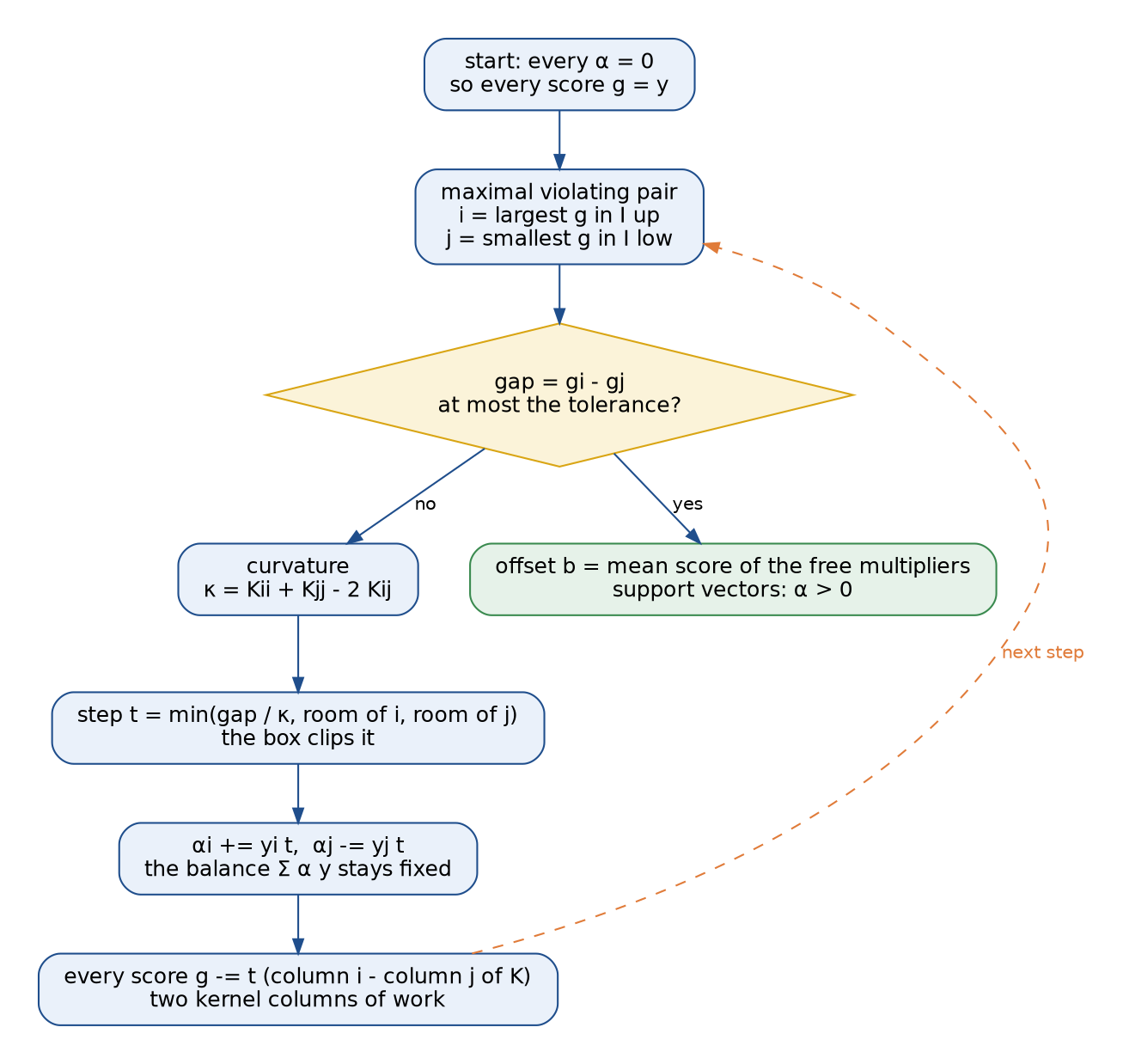
The diagram is the loop of smo in smo.py. LIBSVM refines the choice of j with second-order information, sets aside variables stuck at a bound and caches kernel columns; the version here is the plain first-order method, which keeps every step easy to follow.

How fast is it? On two overlapping Gaussian classes with 500 points each and C = 1, SMO with the linear kernel meets a tolerance of 10⁻⁶ after 2,912 steps. With the RBF kernel and γ = 1 it needs 5,067 steps to reach 10⁻³ and 74,730 to reach 10⁻⁶, most of them spent creeping between the two, which is why LIBSVM's default tolerance is 10⁻³ and why it uses a second-order rule to choose the pair. Pegasos, run for 100,000 single-example steps on the problem with a regularized offset, ends within a relative 7.9 × 10⁻⁵ of the exact optimum for λ = 10⁻² and 9.3 × 10⁻⁵ for λ = 10⁻¹. Its suffix average is at 2.7 × 10⁻⁴ and 1.5 × 10⁻⁵, and its predictions agree with the exact solution on 99.6 % and 100 % of the points.

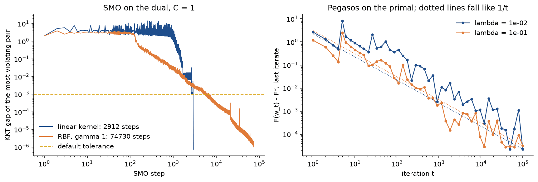
The left panel shows that the RBF run crosses the default tolerance after a few thousand steps and spends the rest of its time on the last three digits. The right panel shows the absolute suboptimality of Pegasos falling roughly like 1/t, as the theory for strongly convex objectives predicts, with large fluctuations from the single-example steps. Both runs come from examples/training_solvers.py.

Kernels

The dual and the decision function touch the inputs only through inner products. Replacing every xᵢᵀxⱼ by a kernel value K(xi, xj) = φ(xi)ᵀφ(xj) trains a maximum-margin hyperplane in the space of φ while computing only kernel values:

The weight vector Σ α y φ(x) lives in the feature space and is never formed. The kernels in common use, with scikit-learn's parameter names (r is coef0 and p is degree):

The linear kernel's feature space is the inputs themselves. The polynomial kernel's contains every monomial up to degree p, and the RBF kernel's is infinite-dimensional. For the degree-two polynomial kernel with γ = 1 and r = 1 in two dimensions the feature map can be written out by expanding the square:

The kernel costs one inner product in two dimensions; the feature map has six coordinates, and for thirty inputs and degree three it would have 5,456. The feature map of the point (1, 2) is (1, 1.4142, 2.8284, 1, 4, 2.8284), and on five random points the explicit inner products agree with the kernel to 4.4 × 10⁻¹⁶. The RBF kernel equals one for identical points and decays to zero with distance; γ = 1 / (2σ²) sets the length scale σ over which a support vector has influence. Expanding its exponential as a power series shows that its feature space contains monomials of every degree.

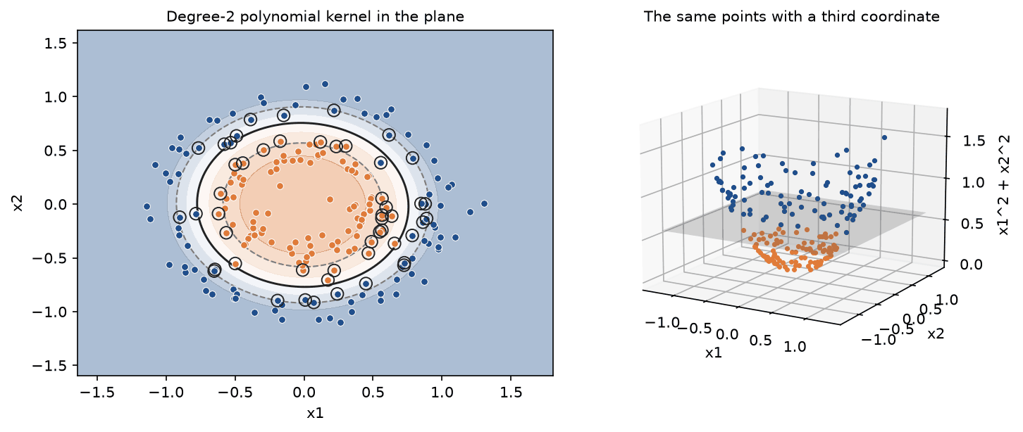
On 200 points of two concentric rings, the linear kernel reaches a test accuracy of 0.5360 on 1,000 fresh points, chance level, while the degree-two polynomial kernel reaches 0.9970 with 50 support vectors. The right panel shows why: the polynomial kernel's feature space contains the squares of both coordinates, and with their sum as a coordinate the rings are separated by a plane.

Mercer's condition

Not every function of two points is an inner product in some space. Mercer's condition, in the form that matters for computation: K is a valid kernel exactly when it is symmetric and every Gram matrix it produces, for any finite set of points, is positive semidefinite:

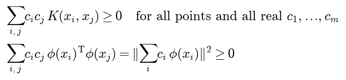
Such a K always has a feature map, and conversely any kernel built from a feature map passes, as the second line shows. The condition is what keeps the dual a concave problem with a single optimum. Sums, products and positive multiples of valid kernels are valid, which is how new kernels are usually built. On thirty random points the smallest Gram eigenvalues of the linear, cubic polynomial and RBF kernels are zero up to rounding (-2.7 × 10⁻¹⁵, -5.4 × 10⁻¹⁴ and 1.1 × 10⁻⁶), while the sigmoid kernel's is -2.24. The sigmoid kernel fails already on the two points (1, 0) and (2, 0) with γ = 1 and r = 0: its Gram matrix has rows (0.7616, 0.9640) and (0.9640, 0.9993), the values of tanh at 1, 2 and 4, and its determinant 0.7616 × 0.9993 - 0.9640² = -0.1683 is negative, so one eigenvalue is negative, -0.0909, the other being 1.8518.

Choosing C and gamma

The RBF kernel has two knobs. γ sets the reach of each support vector: small values give smooth, nearly linear boundaries, large values give each training point its own island. C sets the price of a margin violation: small values give a wide margin with many support vectors, large values chase every training point.

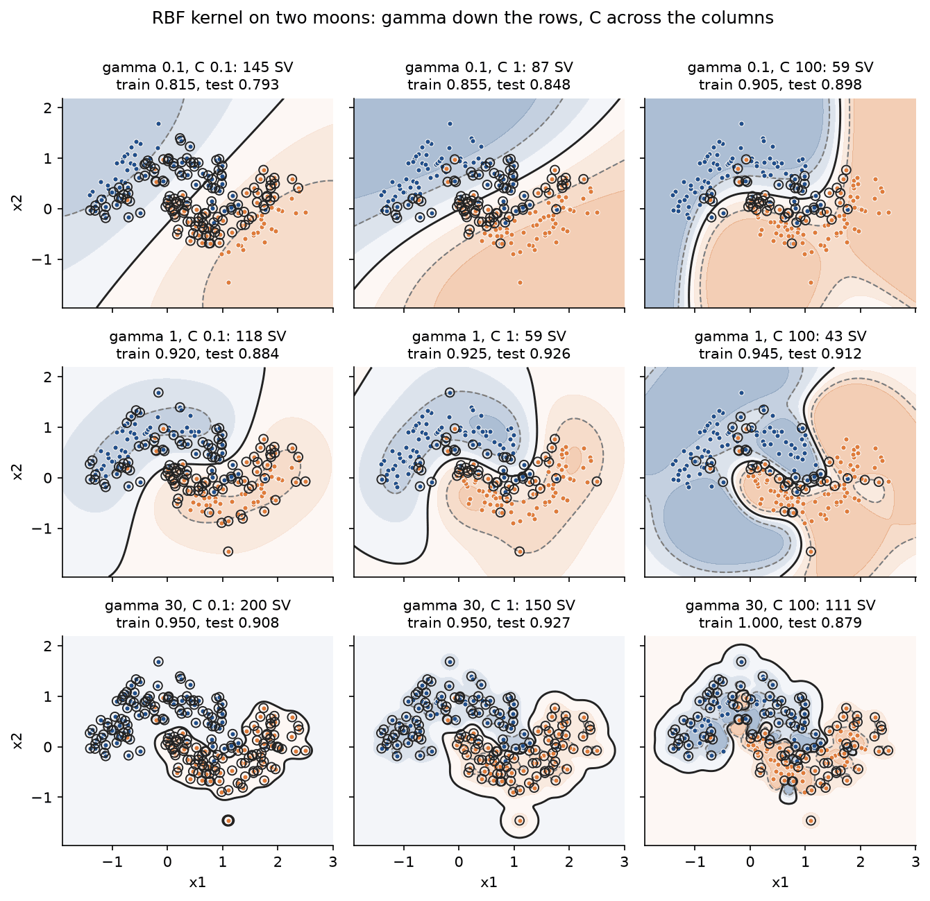
On two moons with noise, 200 training points and 1,000 test points, the nine settings give:

• γ = 0.1: 145, 87 and 59 support vectors for C = 0.1, 1 and 100, with training accuracy 0.815, 0.855 and 0.905 and test accuracy 0.793, 0.848 and 0.898.
• γ = 1: 118, 59 and 43 support vectors, training accuracy 0.920, 0.925 and 0.945, test accuracy 0.884, 0.926 and 0.912.
• γ = 30: 200, 150 and 111 support vectors, training accuracy 0.950, 0.950 and 1.000, test accuracy 0.908, 0.927 and 0.879.

Reading down a column, small γ gives nearly linear boundaries that cannot follow the moons, and large γ gives islands around individual points. Reading along a row, larger C narrows the margin and lowers the number of support vectors. The combination of large γ and large C memorizes the training set: a training accuracy of 1 with the worst test accuracy of the bottom row. With γ = 30 and C = 0.1 every training point is a support vector, but the solution is not overfitted: all 200 multipliers sit at the small bound C, and the classifier is an average of many narrow bumps.

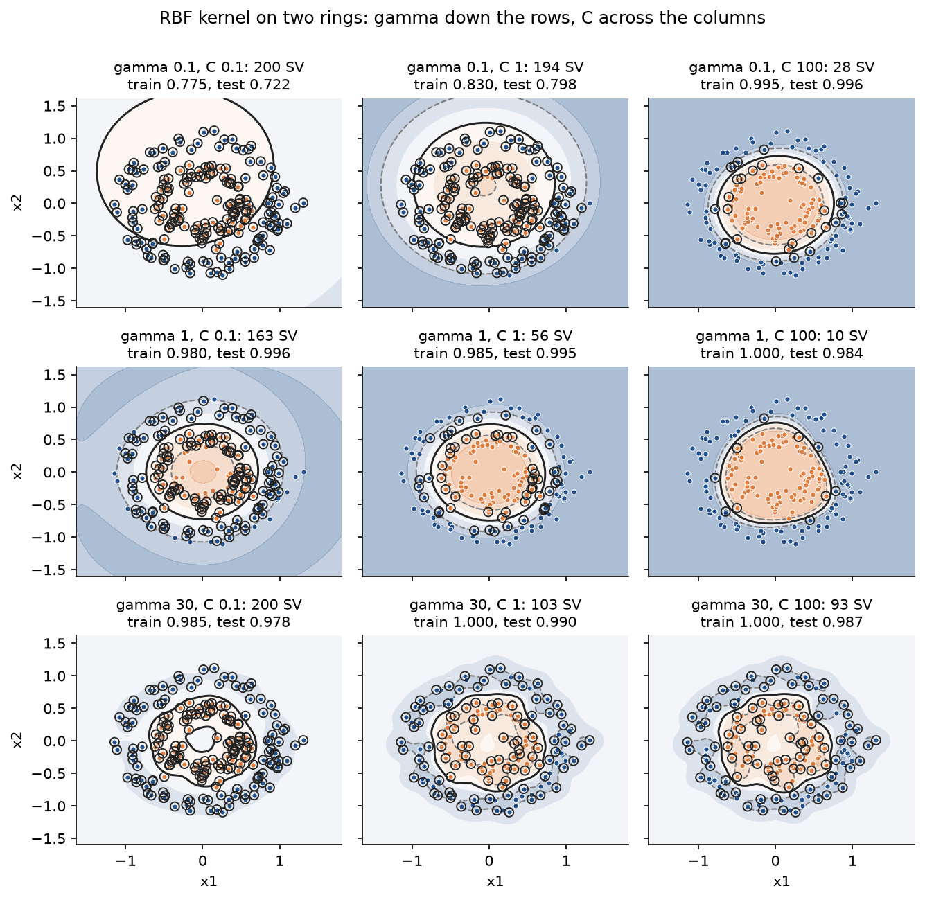
The rings are easier: every setting except the two smoothest, γ = 0.1 with C = 0.1 or 1, exceeds 0.97 on the test set, and with γ = 1 and C = 100 ten support vectors describe the whole boundary.

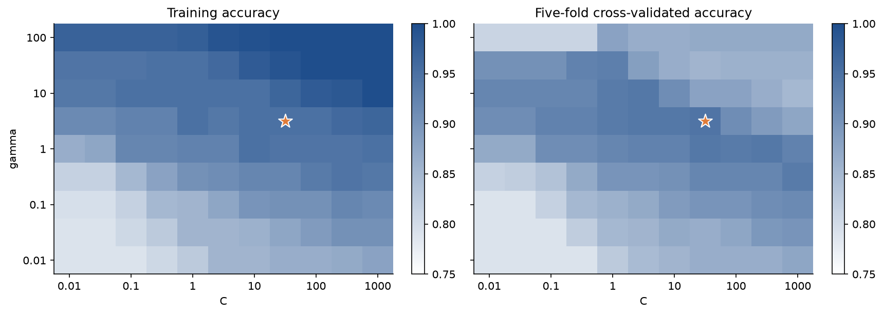
On a finer grid over the moons, 9 values of γ and 11 of C, the best five-fold cross-validated accuracy is 0.9450, at γ = 3.16 and C = 31.6. Training accuracy keeps rising towards the top right of the grid, and the eight settings where it reaches 1 have cross-validated accuracy of only 0.85 to 0.87. The good settings form a diagonal band, because a larger γ needs a smaller C to stay smooth: search the two together on a logarithmic grid.

Multiclass: one-vs-rest and one-vs-one

The machine is binary. For K classes there are two standard reductions:

• One-vs-rest trains K machines, class k against all the others, and predicts the class with the largest decision value. Each machine sees all n points and an imbalanced problem, and the raw outputs are ambiguous where no machine claims a point or several do. The argmax settles those regions by comparing decision values of separately trained machines, which are not on a common scale.
• One-vs-one trains K(K - 1) / 2 machines, one per pair of classes on only those two classes' points, and lets each vote; ties go to the class with the lowest index, as in LIBSVM. More machines, but each is trained on about 2n / K points, and since kernel SVM training grows faster than linearly in n, the total is often cheaper.

scikit-learn's SVC always trains one-vs-one; its decision_function_shape="ovr" turns the pairwise votes and decision values into one score per class but trains no one-vs-rest machines. LinearSVC uses one-vs-rest.

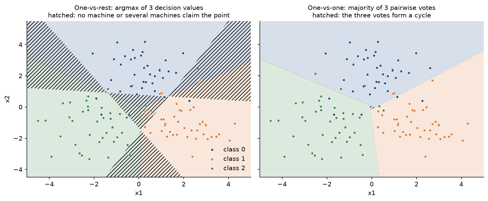
On three overlapping blobs with a linear kernel, both schemes reach the same training accuracy, 0.9083, but draw different regions. Before the argmax, 29.72 % of the plotted square is claimed by no one-vs-rest machine or by several. The three pairwise one-vs-one boundaries nearly meet in a point, and the area where their votes form a cycle is 28 grid points of 90,000.

On the handwritten digits, standardized, with the RBF kernel, γ = 1/64 and C = 10, one-vs-rest trains 10 machines on all 1,347 training images and reaches a test accuracy of 0.9800 on the 450 remaining images. One-vs-one trains 45 machines on 269 images each on average, takes about half the time and reaches 0.9844.

Probabilities: Platt scaling

The decision value ranks points but is not a probability. Platt scaling fits a sigmoid to it,

with A < 0 when larger decision values mean the positive class, by minimizing the cross-entropy on decision values the model did not see during training: a held-out set, or out-of-fold values from cross-validation. Training-set decision values are biased, because the optimization itself pushes them beyond ±1. Platt replaces the targets 1 and 0 by smoothed values, where N₊ and N₋ count each class, so that the fit cannot run off to an infinite slope on separable data:

The two-parameter problem is solved by Newton's method with a backtracking line search. Naive Bayes uses the same recalibration, and Evaluation metrics covers how to judge probabilities.

Scaling

The RBF kernel depends on the squared distance between points, a sum over features, so a feature measured in thousands drowns a feature measured in thousandths, and with raw values every pair of distinct points looks far apart. The linear and polynomial kernels suffer differently: the penalty ‖w‖² treats every coordinate alike, so a feature in large units needs only a tiny weight and is effectively unpenalized while one in small units is penalized heavily, and badly scaled Gram matrices also slow SMO down. Standardizing every feature to zero mean and unit variance, with the mean and variance computed on the training rows only, as in k-nearest neighbours, fixes all three. Fitting the scaler on all rows before splitting is a leak, described in Data leakage and pitfalls.

Worked example

Eight points in the plane, four per class:

• Class -1: point 0 at (2, 0), point 1 at (0, 2), point 2 at (4, 0) and point 3 at (1, 1).
• Class +1: point 4 at (2, 2), point 5 at (3, 3), point 6 at (1, 3) and point 7 at (5, 1).

Every number below is exact, so integers and short decimals are shown as they are; quantities with infinite expansions are rounded to four decimals.

A first guess that fails

The closest pair of opposite points is x3 = (1, 1) and x4 = (2, 2), at distance √2. Guess that they are the only support vectors. The balance condition makes their two multipliers equal, say a, stationarity gives w, and the two active constraints fix a and b:

So w = (1, 1) and b = -3, the perpendicular bisector of the pair. The multipliers are positive, but point 2 has f(x2) = 4 - 3 = 1 and label -1, a functional margin of -1. The functional margins of the eight points are (1, 1, -1, 1, 1, 3, 1, 3): primal feasibility fails, so this is not the solution. The left panel of the figure below shows it.

The right guess

Point 2 has to be on the negative margin, and so, it turns out, does point 1. Guess the support vectors 1, 2 and 4. Their active constraints y (wᵀx + b) = 1 read

Adding the first two gives 2 w1 = 2, so w1 = 1; the third gives b = -1 - 4 = -5; the second gives 2 w2 = -1 + 5, so w2 = 2. Stationarity with w = (1, 2), together with the balance condition, then fixes the multipliers:

All three multipliers are positive. The decision values of the eight points are (-3, -1, -1, -2, 1, 4, 2, 2), so their functional margins are (3, 1, 1, 2, 1, 4, 2, 2) and their geometric margins, divided by √5, are (1.3416, 0.4472, 0.4472, 0.8944, 0.4472, 1.7889, 0.8944, 0.8944). Every functional margin is at least 1, so all five KKT conditions hold and the solution is

• w = (1, 2) and b = -5,
• support vectors 1, 2 and 4,
• multipliers α = (0, 1.5, 1, 0, 2.5, 0, 0, 0).

The boundary is the line x1 + 2 x2 = 5, and the margin hyperplanes are x1 + 2 x2 = 4 through points 1 and 2 and x1 + 2 x2 = 6 through point 4.

Checking the solution

• Width: ‖w‖² = 1 + 4 = 5, so the width is 2 / √5 = 0.8944, and the smallest geometric margin is half of it, 0.4472.
• The identity ‖w‖² = Σ α: 1.5 + 1 + 2.5 = 5.
• Strong duality: the dual objective is Σ α - ‖w‖² / 2 = 5 - 2.5 = 2.5, equal to the primal objective ‖w‖² / 2 = 2.5.
• The offset from each support vector, y - wᵀx: -1 - 4, -1 - 4 and 1 - 6, all -5.
• The margin width with consistent signs: x4 = (2, 2) lies on the positive margin and x2 = (4, 0) on the negative one, and (x4 - x2)ᵀw / ‖w‖ = ((-2) × 1 + 2 × 2) / √5 = 2 / √5 = 0.8944. The reversed difference gives -0.8944.
• An exhaustive search over every candidate set of two or three points with both classes present (hard_margin_by_enumeration) finds points 1, 2 and 4 as the only one that passes.

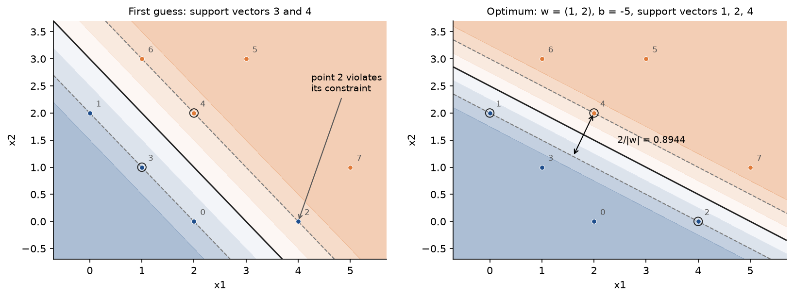
Both panels shade the decision value from blue to orange through white, so the boundary sits where the colour vanishes and the dashed lines are the margins f = -1 and f = +1. In the left panel point 2 lies exactly on the positive margin although it belongs to the negative class.

SMO by hand

The same problem through the dual, with C = ∞ and the linear kernel Kij = xᵢᵀxⱼ. At the start every α is zero, so every u is zero and every score g equals the label. I up holds the positive points, where g = 1, and I low the negative points, where g = -1. The first maximizer and minimizer are i = 4 and j = 0, with gap 2. The curvature is K44 + K00 - 2 K40 = 8 + 4 - 2 × 4 = 4, so the step is 2 / 4 = 0.5, and α4 = α0 = 0.5.

Every u then changes by 0.5 (Kk4 - Kk0), which is 0.5 times the dot product of xk with x4 - x0 = (0, 2), so each u becomes the second coordinate of its point: u = (0, 2, 0, 1, 2, 3, 3, 1) and g = y - u = (-1, -3, -1, -2, -1, -2, -2, 0). Point 0 now has a positive multiplier and joins I up, point 4 joins I low. The maximal violating pair is i = 7, with g7 = 0, and j = 1, with g1 = -3. The steps so far:

• Step 1: pair (4, 0), gap 2, curvature 4, step 0.5, giving α = (0.5, 0, 0, 0, 0.5, 0, 0, 0).
• Step 2: pair (7, 1), gap 3, curvature K77 + K11 - 2 K71 = 26 + 4 - 4 = 26, step 3 / 26 = 0.1154, giving α = (0.5, 0.1154, 0, 0, 0.5, 0, 0, 0.1154).
• Step 3: pair (4, 2), gap 1.3846, curvature 8, step 0.1731, giving α = (0.5, 0.1154, 0.1731, 0, 0.6731, 0, 0, 0.1154).

Point 0, a multiplier that has to end at zero, is clipped to zero at step 7, the first step the box cuts short. The first-order rule then zigzags between two pairs, and the gap shrinks geometrically. It falls below 10⁻¹ after 41 steps, with b = -4.8125, and below 10⁻³ after 81, with α = (0, 1.4993, 0.9995, 0, 2.4988, 0, 0, 0) and b = -4.9978. It falls below 10⁻⁶ after 143 steps and below 10⁻¹² after 267, where the multipliers equal the hand solution to rounding.

Only the support vectors matter

Training on points 1, 2 and 4 alone returns w = (1, 2) and b = -5 again. Leaving out each of the eight points in turn:

• Removing any of the five non-support vectors changes nothing.
• Removing point 1 gives w = (0.5, 1.5) and b = -3.
• Removing point 4 gives w = (0.6667, 1.3333) and b = -3.6667.
• Removing point 2 gives back the first guess, w = (1, 1) and b = -3, under which point 2 is misclassified.

The leave-one-out error is 1 of 8, within the bound of 3 of 8 set by the number of support vectors.

A ninth point: the soft margin

Add the point x8 = (3, 1) with label -1. Under the old classifier f(x8) = 3 + 2 - 5 = 0: it sits exactly on the boundary. The data remain separable, and the new hard margin, found by the same enumeration, tilts to w = (1, 3) and b = -7, with margin hyperplanes x1 + 3 x2 = 6 through points 1 and 8 and x1 + 3 x2 = 8 through points 4 and 7. Its width shrinks to 2 / √10 = 0.6325.

With C = 1 the soft margin refuses to tilt. Its solution keeps the old direction with a wider road:

The margin hyperplanes are x1 + 2 x2 = 4 through points 1 and 2 and x1 + 2 x2 = 7 through points 6 and 7. Point 4 has f(x4) = (2/3) × 6 - 11/3 = 1/3 and the intruder has f(x8) = (2/3) × 5 - 11/3 = -1/3, so both have functional margin 1/3 and slack 2/3 = 0.6667. The three hyperplanes compared on the soft-margin objective with C = 1:

• The old hyperplane, w = (1, 2) and b = -5: penalty ‖w‖² / 2 = 2.5, total slack 1, objective 3.5.
• The new hard margin, w = (1, 3) and b = -7: penalty 5, total slack 0, objective 5.
• The soft margin: penalty 10/9 = 1.1111, total slack 4/3 = 1.3333, objective 22/9 = 2.4444.

To verify optimality, take the multipliers α4 = α8 = C = 1 for the two points inside the margin, α1 = α7 = 0.5 and α2 = α6 = 5/18 = 0.2778 for the four points on it, and zero for the rest. Each class's multipliers sum to 1 + 0.2778 + 0.5 = 1.7778, so the balance condition holds, and stationarity reproduces w:

Every multiplier strictly inside the box belongs to a point with margin exactly 1, both multipliers at C belong to points with margin below 1, and the three points with zero multipliers have margins 7/3, 5/3 and 7/3, all above 1: every one of the three cases holds. These multipliers are what SMO returns, but they are not the only valid ones. Four points on the margin in two dimensions leave one degree of freedom: α1 = 2/9, α2 = 5/9, α6 = 0 and α7 = 7/9 pass the same checks. w and b are unique, the multipliers are not.

With C = 100 the soft margin coincides with the hard margin, with four support vectors on the margin. With C = 0.1 it widens to w = (0.3, 0.5), b = -1.7 and width 3.4300, with eight support vectors, all at the bound, and point 4 now misclassified, with slack 1.1.

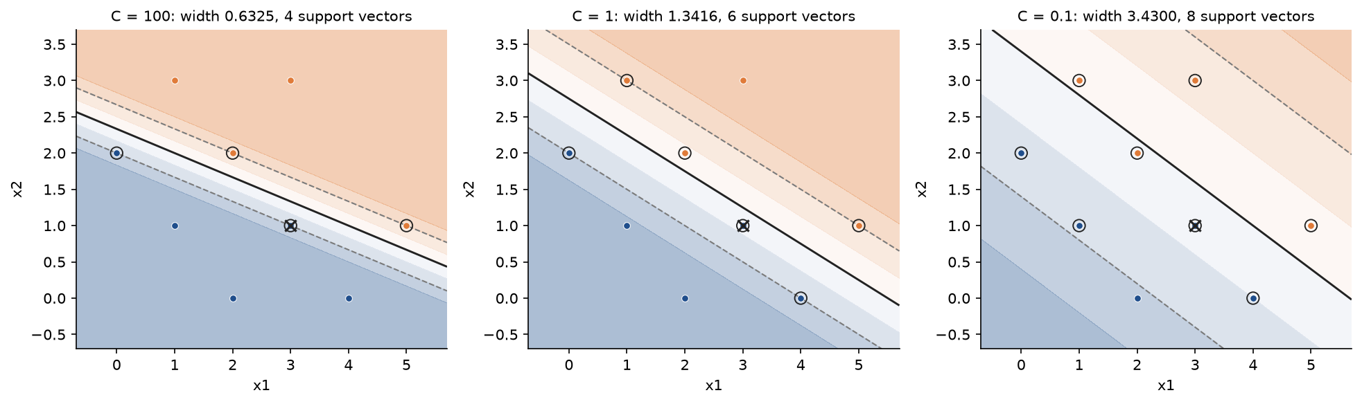
As C falls the road widens and more points stand on it; at C = 0.1 the boundary passes above point 4, the price of a road more than five times wider than the hard margin's.

Every number in this section is asserted by the tests in tests/test_active_set.py, tests/test_smo.py and tests/test_model.py, except the step counts at each tolerance, which depend on the stopping rule and are printed by examples/worked_example.py.

The code

The package support_vector_machines is plain NumPy, split into one module per idea. scikit-learn is imported only inside the data loaders, comparisons.py and pitfalls.py, so everything else works without it.

• arrays.py holds the array types, as_features, which insists on one example per row, and as_signed_labels, which refuses labels other than -1 and +1.
• datasets.py holds the worked example and its ninth point, the synthetic two_moons, concentric_circles and gaussian_blobs, and loaders for the breast cancer and digits data bundled with scikit-learn.
• geometry.py computes decision values, functional and geometric margins, distances, the margin width and the projection behind the sign pitfall.
• losses.py holds the hinge, squared hinge, logistic and 0-1 losses, the slacks, and the primal, regularized-risk and dual objectives.
• active_set.py solves a guessed active set as one linear system and reports a Candidate with its feasibility checks; hard_margin_by_enumeration tries every guess.
• kernels.py holds the four kernels with scikit-learn's parameter names, the Kernel object, the explicit degree-two feature map and the smallest Gram eigenvalue.
• smo.py is the heart of the topic: violating_pair, intercept_from_scores and smo, which can record every step as an SMOStep.
• model.py wraps SMO in fit_svm, returning a KernelSVM with decision_function, predict, the support vectors and their signed multipliers, and audits a solution with kkt_violations and support_categories.
• linear_models.py, pegasos.py and coordinate_descent.py handle the linear machine with a regularized offset: the constant-feature trick, Pegasos and the dual coordinate descent of LIBLINEAR.
• multiclass.py builds OneVsRest and OneVsOne from binary machines.
• platt.py fits Platt scaling by Newton's method and scores probabilities by log loss and the Brier score.
• validation.py holds the Standardizer, stratified splits and folds, cross-validated accuracy with the scaler refitted inside every fold, a grid search over C and γ, out-of-fold decision values and leave-one-out errors.
• comparisons.py builds SVC, LinearSVC, the multiclass wrappers and CalibratedClassifierCV with our settings and measures the agreement.
• pitfalls.py holds deliberately broken or badly configured code for the Pitfalls section.
• plotting.py and boundary_plots.py draw every figure in the handbook's four colours, and threads.py pins the linear algebra libraries to one thread so that results are reproducible.

The loop of smo is the algorithm of the diagram above almost line for line. scores holds the g of every example and starts at the labels, because every multiplier starts at zero:

curvature = gram[first, first] + gram[second, second] - 2.0 * gram[first, second]
curvature = max(curvature, CURVATURE_FLOOR)
room_first = C - alpha[first] if labels[first] > 0 else alpha[first]
room_second = alpha[second] if labels[second] > 0 else C - alpha[second]
step = min(gap / curvature, room_first, room_second)
alpha[first] += labels[first] * step
alpha[second] -= labels[second] * step
scores -= step * (gram[:, first] - gram[:, second])

The real function also snaps a multiplier that reaches a bound exactly onto 0 or C, so that the support vectors can be read off as alpha > 0 without a threshold, and floors the curvature at 10⁻¹² for duplicate points and kernels that are not positive definite.

The examples and the project import the package, so install the repository first as described in the main README. The examples each demonstrate one idea and run from the repository root:

• examples/worked_example.py prints every value of the hard-margin worked example: both guesses, the checks, the enumeration, the first SMO steps, the step counts at each tolerance and the leave-one-out runs.
• examples/soft_margin.py adds the ninth point, compares the three hyperplanes on the soft-margin objective, checks both sets of multipliers and draws the solutions for three values of C and the loss curves.
• examples/training_solvers.py runs SMO and Pegasos on two overlapping blobs of 500 points each and draws their convergence.
• examples/kernels_and_parameters.py checks the feature map and Mercer's condition, separates the rings, and sweeps γ and C on moons and rings, including the finer grid with cross-validation, which takes under a minute.
• examples/multiclass.py draws the regions of both multiclass schemes and runs them on the digits, with the comparison against scikit-learn.
• examples/common_mistakes.py demonstrates the sign swap, labels coded as 0 and 1, a hard margin on overlapping classes, unscaled features and LinearSVC taken for SVC.

python machine-learning/support-vector-machines/examples/worked_example.py
python machine-learning/support-vector-machines/examples/soft_margin.py
python machine-learning/support-vector-machines/examples/training_solvers.py
python machine-learning/support-vector-machines/examples/kernels_and_parameters.py
python machine-learning/support-vector-machines/examples/multiclass.py
python machine-learning/support-vector-machines/examples/common_mistakes.py

The sample project, project/svm_tumour_classifier.py, applies everything to a medical classification task: deciding from 30 measurements of a fine-needle aspirate whether a breast tumour is malignant.

The Breast Cancer Wisconsin data hold 569 tumours, 212 malignant and 357 benign. Each is described by 30 features computed from a digitized image of the aspirate: ten measurements of the cell nuclei, such as radius, texture and concavity, each as a mean, a standard error and a worst value. Malignant is the positive class. A stratified split keeps 25 % of each class for testing, 142 tumours of which 53 are malignant, and the project then follows the diagram. Options such as --seed, --test-fraction, --folds and --tol change the setup, --skip-sklearn leaves out the comparisons, and --figures sends the two PNGs to another folder so a custom run does not overwrite the ones shown here. The default run takes a few seconds.

python machine-learning/support-vector-machines/project/svm_tumour_classifier.py
python machine-learning/support-vector-machines/project/svm_tumour_classifier.py --seed 1 --figures /tmp/svm-figures

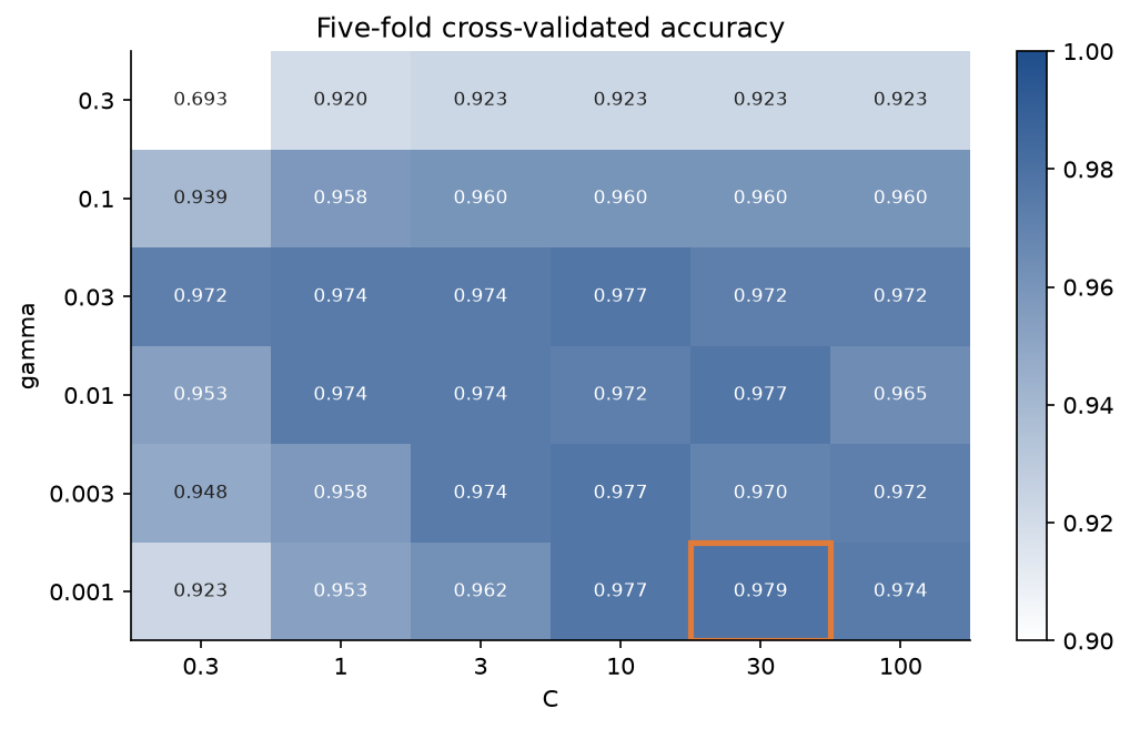
C and γ are chosen by five-fold cross-validation on the 427 training tumours, with the standardizer refitted inside every fold. The best setting, C = 30 and γ = 0.001, scores 0.9789, but ten other settings lie within 0.005 of it, about two tumours out of 427, so the choice among them is close to noise. Only the largest γ with the smallest C falls apart, at 0.6933. Refitted on all training tumours with tolerance 10⁻⁶, the model has 55 support vectors: 12 on the margin, 36 inside it and 7 misclassified training tumours. On the test set it reaches an accuracy of 0.9718, finding 50 of the 53 malignant tumours and calling 1 of the 89 benign ones malignant.

Platt scaling fitted on out-of-fold decision values from the same five folds gives A = -2.5990 and B = -0.1608. The calibrated probabilities have a test log loss of 0.1173 and a Brier score of 0.0274; a plain sigmoid of the decision value, without fitting, has a log loss of 0.1844.

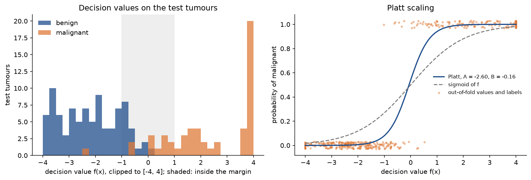
The histogram shows the few test tumours that fall inside the margin, where the errors are, and the right panel shows why the plain sigmoid is too timid: the out-of-fold values separate the classes more sharply than a slope of one suggests.

The notebook support_vector_machines.ipynb is a guided tour in the order of this page: the worked example by guessing, by enumeration and by SMO, the soft margin on the nine points, SMO and Pegasos on more data, kernels and Mercer's condition, the C and γ sweep, the multiclass schemes, each pitfall, the tumour classifier and the comparison with scikit-learn. The tests in tests check the worked example value by value, the mathematical properties above and the agreement with scikit-learn, and run in a few seconds:

python -m pytest machine-learning/support-vector-machines

Data:

• Breast Cancer Wisconsin (Diagnostic), by W. H. Wolberg, O. L. Mangasarian, W. N. Street and W. Street, from the UCI Machine Learning Repository (1995), licensed CC BY 4.0. scikit-learn ships a copy as sklearn.datasets.load_breast_cancer, so nothing is downloaded.
• Optical Recognition of Handwritten Digits, by E. Alpaydin and C. Kaynak, from the UCI Machine Learning Repository (1998), licensed CC BY 4.0. scikit-learn's load_digits contains 1,797 of its images of 8 by 8 pixels.
• The moons, rings and blobs are synthetic, generated by the package from fixed seeds.

In practice

SVC wraps LIBSVM, which solves the same dual with an SMO-type method. Fitted on the standardized training tumours with the same settings and tolerance 10⁻⁶ on both sides, the two agree as follows (decision values on the test tumours):

• RBF, C = 30, γ = 0.001: largest decision difference 2.4 × 10⁻⁵, the same support vectors, largest dual coefficient difference 4.0 × 10⁻³, intercept difference 3.6 × 10⁻⁵.
• Linear, C = 1: decision difference 1.3 × 10⁻⁵, the same support vectors, dual coefficient difference 2.4 × 10⁻⁶, intercept difference 1.2 × 10⁻⁷.
• Polynomial of degree 3 with γ = 1/30 and r = 1, C = 1: decision difference 4.1 × 10⁻⁶, the same support vectors, dual coefficient difference 1.3 × 10⁻⁵, intercept difference 9.5 × 10⁻⁷.

The same comparison on any data takes three lines:

from support_vector_machines import Kernel, compare_with_sklearn, fit_svm, two_moons

points, labels = two_moons(60, noise=0.25, seed=3)
model = fit_svm(points, labels, C=2.0, kernel=Kernel("rbf", gamma=2.0), tol=1e-10)
print(compare_with_sklearn(model, points, labels, points, tol=1e-10))

The support vectors coincide exactly. Agreement stops near 10⁻⁵ for two reasons: a tolerance on the KKT gap does not bound the error in decision values tightly, and LIBSVM stores kernel values in its cache in single precision, so its own solution carries errors of about 10⁻⁷ relative whatever the tolerance. Tightening both tolerances to 10⁻¹⁰ or 10⁻¹² leaves the largest test decision difference for the RBF model at 2.2 × 10⁻⁵, while our own solutions at those two tolerances agree to 2.5 × 10⁻¹⁰. The dual coefficients of the RBF model differ more than its decision values because with γ = 0.001 the Gram matrix is nearly singular, so very different multipliers produce almost the same function. The tests compare at tolerance 10⁻¹⁰ on small problems with three kernels (test_smo_matches_svc) and at 10⁻⁶ on the full breast cancer data. LIBSVM is several times to tens of times faster than our NumPy loop on these problems.

LinearSVC(loss="hinge") wraps LIBLINEAR's dual coordinate descent, the method in dual_coordinate_descent: the offset is the weight of a constant feature, so there is no balance condition and one multiplier can be optimized at a time in closed form. On the standardized training tumours with C = 1, both reach the objective 13.673293, their test decision values differ by at most 2.9 × 10⁻⁸, and the 27 support vectors read off LIBLINEAR's decision values as the points with y f(x) ≤ 1 are exactly the 27 points with α > 0. Pegasos's suffix average after 100,000 steps reaches 14.007501, 2.4 % above the optimum, and a test accuracy of 0.9437 against 0.9507: λ = 1/427 is small, and small λ is where Pegasos is slow.

The multiclass wrappers agree as well. With the tolerance tightened to 10⁻⁶ on both sides, our one-vs-one predictions on the digits equal those of SVC on every test image, with pairwise decision values within 1.1 × 10⁻⁶, and our one-vs-rest predictions equal those of OneVsRestClassifier(SVC(...)), with decision values within 1.6 × 10⁻⁶. For probabilities, CalibratedClassifierCV with method="sigmoid", ensemble=False, the same folds and a StandardScaler and SVC pipeline gives tumour probabilities within 1.2 × 10⁻⁵ of ours.

When to use which:

• Up to some tens of thousands of examples, use SVC with the RBF kernel on standardized features and search C and γ together on a logarithmic grid, inside cross-validation. gamma="scale", one over the number of features times the variance of all feature values, is a sensible centre for the grid.
• For many examples or many sparse features, as in text, use a linear model: LinearSVC or SGDClassifier(loss="hinge"), the Pegasos family. Kernel SVM training grows between quadratically and cubically with n and needs the kernel matrix or a cache of it, and prediction costs one kernel evaluation per support vector.
• To get nonlinear boundaries at linear cost, approximate the kernel with explicit random features (RBFSampler, Nystroem) and train a linear model on them.
• When calibrated probabilities matter, wrap the model in CalibratedClassifierCV(..., method="sigmoid"); SVC(probability=True) does the same internally and is deprecated as of scikit-learn 1.9. When probabilities are the main goal, logistic regression gives them directly.
• Use the from-scratch code to understand what the library is doing, to inspect multipliers and KKT conditions, and to experiment with solvers; it is not a replacement for LIBSVM.

Pitfalls

• A sign swap in the margin derivation. The width is the projection of x₊ - x₋ onto the unit normal with x₊ on f = +1 and x₋ on f = -1. Derivations sometimes substitute each point into the other's equation, or subtract in one order and project in the other, and arrive at -2 / ‖w‖, or patch the sign without noticing. In the worked example the projection of x4 - x2 is 0.8944 and that of x2 - x4 is -0.8944 (examples/common_mistakes.py, tests/test_geometry.py).
• Labels coded as 0 and 1. Every formula assumes labels -1 and +1. With y = 0 the hinge loss is the constant 1, its subgradient vanishes and the negative class exerts no force: a hand-written subgradient descent on two balanced blobs then predicts the positive class for 99.5 % of the points instead of 50 %. The package refuses such labels (tests/test_arrays.py), and examples/common_mistakes.py runs the broken version.
• Unscaled features. On the raw breast cancer features, whose standard deviations on the training tumours range from 0.0026 to 555.0, the RBF kernel with γ = 1/30 makes all 427 training tumours support vectors, memorizes them, and scores 0.6268 on the test set, exactly the share of benign tumours: every one of the 142 test tumours is called benign. After standardization it uses 101 support vectors and scores 0.9789. Fit the scaler on the training rows only.
• LinearSVC is not SVC with a linear kernel. LinearSVC() minimizes the squared hinge loss and regularizes the offset. On the standardized breast cancer data its test decision values differ from SVC(kernel="linear") by up to 6.8147 and its weights by up to 0.4803; with loss="hinge" the differences drop to 0.0020 and 0.0004, and the rest is the regularized offset, which intercept_scaling controls.
• A hard margin on overlapping classes. Without slack the primal has no feasible point and the dual is unbounded. On the moons, SMO with C = ∞ keeps a KKT gap of about 3.3 while the largest multiplier grows from 260.8 after 1,000 steps to 1,303.7 after 5,000 and 5,214.6 after 20,000 (examples/common_mistakes.py). Use a finite C, and treat huge multipliers as a sign of it.
• Judging a setting by training accuracy. With γ = 30 and C = 100 every moons training point is classified correctly and test accuracy is the lowest of its row, 0.879; on the finer grid, the settings with training accuracy 1 have cross-validated accuracy 0.85 to 0.87 against the best 0.9450. Choose C and γ by cross-validation and keep the test set for the end.
• Treating the sigmoid kernel as a kernel. tanh ranges over (-1, 1), not (0, 1), and the sigmoid kernel is not positive semidefinite: the two-point Gram matrix under Mercer's condition has eigenvalue -0.0909, and on thirty random points the smallest eigenvalue is -2.24 (tests/test_kernels.py). The dual is then not concave and solvers may stop at different points; the kernel is offered mainly for its resemblance to a neural network layer.
• Reading decision values as probabilities. A plain sigmoid of the decision value gives a test log loss of 0.1844 on the breast cancer data, Platt scaling 0.1173. Fit Platt scaling on held-out or out-of-fold decision values, never on the training values, which the optimization has pushed beyond ±1. Thresholding the calibrated probability at 0.5 corresponds to f = -B/A rather than f = 0, so the two decisions can differ near the boundary; on this test set none did. With SVC(probability=True) the probabilities come from an internal cross-validation and can disagree with predict for the same reason.
• Expecting unique multipliers. w, b and the decision function are unique when the kernel is positive definite, but the multipliers need not be: with the ninth point, two different sets of multipliers satisfy every KKT condition (examples/soft_margin.py), and on the breast cancer RBF model our dual coefficients and LIBSVM's differ by up to 4.0 × 10⁻³ while the decision values agree to 2.4 × 10⁻⁵. Compare solvers on decision values and support vectors, and remember that scikit-learn's dual_coef_ holds α y, not α.
• Fitting the scaler, or anything else, before cross-validation. A scaler, a feature selector or a choice of γ made on all rows lets the held-out folds influence training. cross_validated_accuracy refits the standardizer inside every fold, and the tumour project chooses C and γ on the training rows only; Data leakage and pitfalls measures how much the shortcut inflates scores.

Further reading

• B. E. Boser, I. M. Guyon and V. N. Vapnik, "A training algorithm for optimal margin classifiers", Proceedings of the Fifth Annual Workshop on Computational Learning Theory, 144-152, 1992. The maximum-margin classifier with kernels.
• C. Cortes and V. Vapnik, "Support-vector networks", Machine Learning 20(3), 273-297, 1995. The soft margin.
• J. C. Platt, "Sequential minimal optimization: a fast algorithm for training support vector machines", Microsoft Research technical report MSR-TR-98-14, 1998.
• S. S. Keerthi, S. K. Shevade, C. Bhattacharyya and K. R. K. Murthy, "Improvements to Platt's SMO algorithm for SVM classifier design", Neural Computation 13(3), 637-649, 2001. The maximal violating pair and the two-threshold stopping rule used here.
• R.-E. Fan, P.-H. Chen and C.-J. Lin, "Working set selection using second order information for training support vector machines", Journal of Machine Learning Research 6, 1889-1918, 2005.
• C.-C. Chang and C.-J. Lin, "LIBSVM: a library for support vector machines", ACM Transactions on Intelligent Systems and Technology 2(3), 27:1-27:27, 2011.
• C.-J. Hsieh, K.-W. Chang, C.-J. Lin, S. S. Keerthi and S. Sundararajan, "A dual coordinate descent method for large-scale linear SVM", Proceedings of the 25th International Conference on Machine Learning, 2008.
• S. Shalev-Shwartz, Y. Singer, N. Srebro and A. Cotter, "Pegasos: primal estimated sub-gradient solver for SVM", Mathematical Programming 127(1), 3-30, 2011.
• A. Rakhlin, O. Shamir and K. Sridharan, "Making gradient descent optimal for strongly convex stochastic optimization", Proceedings of the 29th International Conference on Machine Learning, 2012. Suffix averaging.
• J. C. Platt, "Probabilistic outputs for support vector machines and comparisons to regularized likelihood methods", in Advances in Large Margin Classifiers, MIT Press, 1999.
• H.-T. Lin, C.-J. Lin and R. C. Weng, "A note on Platt's probabilistic outputs for support vector machines", Machine Learning 68(3), 267-276, 2007. The Newton method used by fit_platt_scaling.
• C.-W. Hsu and C.-J. Lin, "A comparison of methods for multiclass support vector machines", IEEE Transactions on Neural Networks 13(2), 415-425, 2002.
• C.-W. Hsu, C.-C. Chang and C.-J. Lin, "A practical guide to support vector classification", technical note, National Taiwan University, 2003. Scaling and grid search in practice.
• B. Schölkopf and A. J. Smola, Learning with Kernels, MIT Press, 2002.
• S. Boyd and L. Vandenberghe, Convex Optimization, chapter 5, Cambridge University Press, 2004. Lagrange duality and the KKT conditions.
• C. M. Bishop, Pattern Recognition and Machine Learning, chapter 7, Springer, 2006.
• W. N. Street, W. H. Wolberg and O. L. Mangasarian, "Nuclear feature extraction for breast tumor diagnosis", IS&T/SPIE International Symposium on Electronic Imaging, 1993. The origin of the breast cancer features.