Retrieval-augmented generation

A language model answers from what its weights absorbed during training, and when that memory is missing, outdated or mixed up it still produces a fluent answer. Retrieval-augmented generation gives the model a second memory it can read: the question is first used to search a document collection, the passages found are placed in the prompt as numbered sources, and the model is asked to answer from them and cite them, so every claim can be traced and checked. This page builds such a system from scratch: chunking documents three ways, sparse retrieval with tf-idf and BM25, dense retrieval with latent semantic analysis, exact and approximate vector search, hybrid ranking with reciprocal rank fusion, prompt assembly with citation checking, and a small generator that runs offline. It derives the RAG-Sequence and RAG-Token formulations, works one query through every stage by hand, and measures every stage on 64 labelled questions over ten encyclopedia articles. Afterwards you will be able to build and evaluate a retrieval pipeline, choose chunk sizes and retrievers by measurement rather than habit, and detect answers that their sources do not support. It builds on Text representations for tf-idf and on Dimensionality reduction for the singular value decomposition behind LSA.

To run the code in this topic, install the base group, the ml group for the comparison with scikit-learn and the nlp group for the token counts with tiktoken.

Intuition

A model's weights are a lossy, frozen summary of its training text, its parametric memory. A document collection is an exact, editable memory, but a model cannot read millions of pages for every question. Retrieval bridges the two: a cheap search narrows the collection to a few passages, and the expensive model reads only those. The system therefore lives or dies by the passages it retrieves, and most of the engineering, and most of this page, is about finding the right ones and checking that the answer really came from them.

The diagram shows the two halves. Indexing happens once per collection: the documents are cut into chunks, and each chunk enters an inverted index for word matching and, after an encoder has turned it into a vector, a vector index. Answering happens once per question: both indexes are searched, the two rankings are fused, the best chunks become the sources of a prompt, and the answer is checked against the sources it cites.

Each stage has a characteristic failure, and each failure looks the same from the outside: a confident answer that is wrong.

• Chunking decides what a passage is. Too small, and a chunk loses its subject ("It takes 87.969 Earth days to complete an orbit." never says which planet) or the evidence is cut in two. Too large, and each chunk costs many prompt tokens and its score is diluted by unrelated text.
• Sparse retrieval matches words. It is precise for names and numbers and blind to paraphrase: "How long is a year on Venus?" shares no content word with "completes an orbit every 224.7 days".
• Dense retrieval matches meaning through vectors learned from co-occurrence, so it can bridge vocabulary gaps, at the price of sometimes ranking a chunk about the right topic above the chunk with the answer.
• Fusion combines the two using ranks only, so neither score scale dominates.
• The generator can ignore its sources and answer from parametric memory. The citation and support checks exist to catch that, and the Pitfalls section shows a case where they do.

How it works

Notation

The collection holds N chunks. A chunk is d and the question, or query, is q. A term t is a word kept by the analyzer after lowercasing, stripping accents and dropping stopwords. The formula images write the count of term t in chunk d as f with the subscripts t and d, the number of chunks that contain t, its document frequency, as n with subscript t, the length of chunk d in terms as |d| and the average length as ℓ with a bar. In the text these are simply the count f, the document frequency n, the length |d| and the average length. BM25 has two parameters, k1 for saturation and b for length normalization, 1.5 and 0.75 here. Retrieval returns the k best chunks, and the fusion constant, k in the code, is c in the formulas. The generator receives an input x and produces an answer y of m tokens, y1 to ym, and a retrieved chunk is written z when it is treated as a hidden variable.

Chunking and how often a window cuts the evidence

A chunker maps a document to a list of character ranges. Three are implemented. Fixed windows take W consecutive words and advance by a stride s = W - o, where o is the overlap. Sentence chunks pack whole sentences into a chunk until the next sentence would exceed a word limit, and never cross a section boundary. Section chunks are the sections themselves.

Relevance is defined independently of the chunker. Each question is labelled with evidence spans, the exact text that answers it, and a chunk is relevant when it contains a whole span. If a span occupies the characters from e with subscript s to e with subscript e, and a chunk the characters from d with subscript s to d with subscript e, the chunk contains the span when

so the same labels can judge every chunking strategy.

How often does a fixed window cut a span of L words, with L at most W? Windows start at every multiple of the stride. Let ρ be the distance from the last window start at or before the span to the span's first word, a number from 0 to s - 1. That window contains the span exactly when ρ + L ≤ W; an earlier window ends sooner and a later one starts after the span begins. For a span at a random position ρ is uniform, which gives

Without overlap a span is cut with probability (L - 1)/W, and an overlap of at least L - 1 words guarantees that some window contains it whole. The 68 pieces of evidence in the question set average 11.25 words and the longest span has 30, so an overlap of 29 words makes cuts impossible. For 100-word windows without overlap the formula expects 4.7 cut pieces, counting a piece as cut only when every one of its alternative spans is, and the corpus has 3.

Sparse retrieval: tf-idf

The tf-idf weight of term t in chunk d is a term-frequency factor times an inverse document frequency:

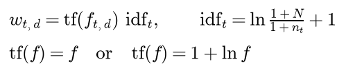
The idf is scikit-learn's smoothed form: the added ones act as if one extra chunk contained every term, so no idf divides by zero, and the final one keeps terms that occur everywhere from vanishing. Sublinear scaling makes the tenth occurrence of a word worth far less than the first. A query gets weights the same way, and the score is the cosine of the angle between the two weight vectors:

The division by the lengths matters: without it a long chunk scores higher simply because it contains more terms.

Sparse retrieval: BM25

BM25 scores a chunk by summing, over the distinct query terms, an idf weight times a saturating function of the term count:

with the idf

The idf comes from the probabilistic model of relevance. Suppose a term occurs in a relevant chunk with probability p and in a non-relevant one with probability u. Observing it then shifts the log-odds of relevance by the first line below. Without any relevance judgements, take p = 1/2 and estimate u from the whole collection as n/N; adding 0.5 to each count to avoid zeros gives the Robertson and Spärck Jones weight on the third line:

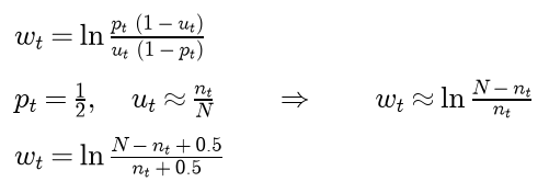
That weight is negative for a term in more than half the chunks, which punishes a chunk for containing a query word. Adding one inside the logarithm, as Lucene does and as the code here does, keeps it positive.

The second factor saturates. It is 0 when the term is absent, grows with the count, and never exceeds k1 + 1, so the tenth occurrence of a word adds far less than the first; k1 sets how fast the curve flattens. K grows with the chunk's length relative to the average, so the same count is worth less in a long chunk, and b sets how strongly: b = 0 ignores length and b = 1 normalizes fully. For a chunk of average length K equals k1, and one occurrence contributes exactly the idf.

Dense retrieval with latent semantic analysis

Write the tf-idf matrix X, one unit-length row per chunk and one column per term, as a singular value decomposition with the singular values in decreasing order. Keeping the first r columns of U and V and the first r singular values gives the closest matrix of rank r to X in the Frobenius norm, by the Eckart and Young theorem. Latent semantic analysis embeds a chunk by projecting its row onto the r right singular vectors, and a query the same way:

The rows of V r times Σ r embed the terms. Two terms that occur in similar chunks get similar rows even if they never occur together, which is how a question can reach a chunk that shares few of its words. With r equal to the rank of X nothing is lost and the ranking equals the tf-idf ranking, which a test checks; a small r merges terms, which helps with paraphrase and hurts with rare, distinctive words. Terms found in a single chunk carry no co-occurrence information, so the matrix keeps only terms with a document frequency of at least two.

Exact and approximate nearest-neighbour search

With unit vectors, cosine similarity is a dot product, and exact search multiplies the matrix of chunk embeddings by the query embedding and keeps the k largest entries: N times r operations per query. An inverted-file index (IVF) avoids scanning everything. It partitions the vectors into L lists with spherical k-means, which for unit vectors minimizes

so each round gives every vector to the centroid with the largest dot product and replaces each centroid by the normalized sum of its vectors.

At query time the query is compared with the L centroids, the p closest lists are scanned exactly, and the best k candidates are returned. With balanced lists a query costs about L + pN/L dot products, which is smallest when L is about the square root of pN:

The price is recall: a true neighbour that was assigned to a list that was not probed is missed. The quality of an approximate index is measured against exact search, with A the approximate and E the exact top k, averaged over queries:

This says nothing about relevance; that is what the labelled metrics below are for.

Hybrid ranking with reciprocal rank fusion

BM25 scores are unbounded and grow with query length, while cosine similarities lie between -1 and 1, so adding the two lets the larger scale decide. Reciprocal rank fusion uses only the rank of chunk d in each list j that contains it:

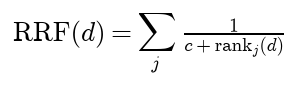
With the usual c = 60, rank 1 contributes 1/61 and rank 2 contributes 1/62, almost the same, so a chunk that both retrievers place fairly high beats one that a single retriever places first. A small c makes the top ranks count more. Ties are broken by chunk id so the result is deterministic.

Prompt assembly and citation checking

The prompt is an instruction, the retrieved chunks as numbered sources each labelled with its article and section, and the question. Given a token budget, it takes the longest prefix of the ranked list that fits, so a lower-ranked chunk never displaces a higher-ranked one.

A claim is a sentence of the answer. With T(s) the analyzed terms of sentence s, citation markers removed, and T(S) the terms of the sources it cites, its support is the share of its terms, counting repeats, that occur in those sources:

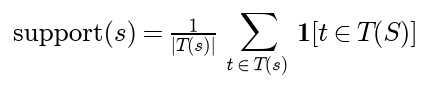
A claim passes when it cites at least one existing source, its support is at least 0.75, and every number in it occurs in the cited sources. This is a lexical stand-in for entailment: it catches invented numbers and citations to the wrong source, it cannot see negation or paraphrase, and it says nothing about whether the claim answers the question.

An extractive generator

The offline generator answers with one sentence from the sources. Let Q be the analyzed question terms, after dropping the word that follows "how", as in "how long", which rarely occurs in the answer, and H(s) the terms of the label of the source that holds sentence s. Each sentence is scored by the share of the question's idf weight it covers:

Half a point is subtracted when a "how many", "how long" or "when" question meets a sentence without a number. The best sentence is returned with its citation, or the generator abstains when the coverage is below a threshold. Every answer is a verbatim quotation, so it can never invent a number, but it can quote the wrong sentence.

RAG-Sequence and RAG-Token

Lewis and colleagues treat the retrieved chunk as a hidden variable and add up over the top k chunks. The retriever's distribution is a softmax of the retrieval scores, with a temperature τ:

In their model the score is the inner product of a query encoder and a document encoder. The two formulations differ in when the sum over chunks happens. RAG-Sequence uses one chunk for the whole answer:

RAG-Token may use a different chunk for every token:

The difference becomes clear when RAG-Sequence is also written as a product over tokens. Let a with subscripts z and i be the generator's probability of token i under chunk z, and P with subscript i the RAG-Sequence probability of the first i tokens, so that the probability of the whole answer is P with subscript m. Writing it as a product of ratios shows what each factor is:

So RAG-Sequence is a mixture whose weights are updated by Bayes' rule after every token: as the answer unfolds it commits to the chunks that explain it. RAG-Token keeps the prior weights at every step. That is why RAG-Token can assemble an answer from facts in different chunks, and also why it can attach a fact from one chunk to the subject of another.

Training maximizes the log-likelihood of the answer under either formulation, and gradients reach the query encoder through the retriever's distribution, so the retriever learns which chunks help the generator; the document encoder and its index stay fixed. Decoding differs: RAG-Token is an ordinary beam search over the mixed next-token distribution, while RAG-Sequence runs a beam search per chunk and then scores every hypothesis under every chunk. The examples and the notebook compute both likelihoods for a trigram generator conditioned on retrieved chunks.

Measuring retrieval

A question has g pieces of evidence, and G with subscript j is the set of chunks that contain piece j, or one of its alternative spans. For a ranking d1, d2 and so on, recall at k counts the pieces found in the top k, and the reciprocal rank is one over the rank of the first relevant chunk, or zero when none is ranked:

The mean reciprocal rank, MRR, averages RR over questions. With a gain g(d) of at least zero for each chunk, the discounted cumulative gain and its normalized form are

where the ideal DCG is the DCG of the best possible ranking of the whole collection. On the corpus every relevant chunk has gain 1; the worked example uses graded gains. Recall at k asks whether the evidence reached the prompt, MRR how early, and nDCG rewards putting the most useful chunks first.

Worked example

Four chunks and the question "What moons does Mars have?". The analyzer lowercases, drops stopwords and keeps words and numbers:

• d1, "Mars has two small moons, Phobos and Deimos.", has the six terms mars, two, small, moons, phobos and deimos.
• d2, "Phobos orbits Mars faster than Mars rotates.", has the six terms phobos, orbits, mars, faster, mars and rotates.
• d3, "Jupiter has dozens of moons, including four large moons.", has the seven terms jupiter, dozens, moons, including, four, large and moons.
• d4, "The red colour of Mars comes from iron oxide dust.", has the seven terms red, colour, mars, comes, iron, oxide and dust.

The question becomes the two terms moons and mars. Every value below is computed in double precision and shown to four decimals; where a sum written out from rounded terms differs from the full-precision value in the last digit, the text says so.

BM25

There are N = 4 chunks, moons occurs in 2 of them and mars in 3, and the average length is 26/4 = 6.5 terms, with k1 = 1.5 and b = 0.75.

• The idf of moons is ln(5/2.5) = ln 2 = 0.6931, and the idf of mars is ln(5/3.5) = 0.3567.
• The length factor K is 1.5 × (0.25 + 0.75 × 6/6.5) = 1.4135 for the six-term chunks and 1.5 × (0.25 + 0.75 × 7/6.5) = 1.5865 for the seven-term ones.
• The saturating factor f(k1 + 1)/(f + K) is 2.5/2.4135 = 1.0359 for one occurrence in a short chunk, 5/3.4135 = 1.4648 for two (mars in d2), 5/3.5865 = 1.3941 for two in a long chunk (moons in d3) and 2.5/2.5865 = 0.9665 for one in a long chunk.
• Multiplying by the idf, moons contributes 0.7180 to d1 and 0.9663 to d3, and mars contributes 0.3695 to d1, 0.5225 to d2 and 0.3447 to d4.
• The scores are 1.0875 for d1, 0.5225 for d2, 0.9663 for d3 and 0.3447 for d4, so BM25 ranks d1, d3, d2, d4.

Two occurrences of mars in d2 are worth 0.5225, not twice 0.3695, because of the saturation.

tf-idf and a dense encoder

With the smoothed idf, mars gets ln(5/4) + 1 = 1.2231, moons gets ln(5/3) + 1 = 1.5108, and every term found in a single chunk gets ln(5/2) + 1 = 1.9163. The chunk vectors have lengths 4.1325, 4.3913, 5.2432 and 4.8507, the query vector has length √(1.2231² + 1.5108²) = 1.9439, and the dot products with the query are 3.7787, 2.9922, 4.5652 and 1.4961. For d1 the cosine is 3.7787 / (4.1325 × 1.9439) = 0.4704; all four are 0.4704, 0.3505, 0.4479 and 0.1587, the same order as BM25.

A dense encoder is represented by two-dimensional embeddings: (0.8, 0.6) for the query, and (0.5, 0.9), (1.0, 0.5), (-0.1, 1.0) and (0.9, -0.2) for d1 to d4. The query has unit length, so each cosine is the dot product divided by the chunk's length: for d2, (0.8 + 0.3)/1.1180 = 0.9839. The four cosines are 0.9130, 0.9839, 0.5174 and 0.6508, a ranking d2, d1, d4, d3 that puts the chunk about Phobos first and the Jupiter chunk last.

Fusion and evaluation

Reciprocal rank fusion with c = 10, small enough that the ranks visibly matter (60 is the usual default), combines the two rankings:

d1 is first for BM25 and second for the dense encoder and gets 1/11 + 1/12 = 0.1742; d2 gets 1/13 + 1/11 = 0.1678, d3 gets 1/12 + 1/14 = 0.1548 and d4 gets 1/14 + 1/13 = 0.1484. Added from the rounded terms, 0.0833 + 0.0714 and 0.0714 + 0.0769 give 0.1547 and 0.1483; at full precision they are 0.1548 and 0.1484. The fused ranking is d1, d2, d3, d4.

For the labels, d1 answers the question (gain 2), d2 is about one of the moons (gain 1), and d3 and d4 are irrelevant; each relevant chunk is its own piece of evidence, so g = 2. The ideal ranking d1, d2 has an ideal DCG@3 of 2/log2(2) + 1/log2(3) = 2 + 0.6309 = 2.6309.

• BM25, ranking d1, d3, d2: recall 0.5, 0.5 and 1.0 at k = 1, 2 and 3, reciprocal rank 1.0, DCG@3 = 2 + 0 + 1/2 = 2.5000 and nDCG@3 = 0.9502.
• Dense, ranking d2, d1, d4: recall 0.5, 1.0 and 1.0, reciprocal rank 1.0, DCG@3 = 1 + 2/1.5850 = 2.2619 and nDCG@3 = 0.8597.
• Fused, ranking d1, d2, d3: recall 0.5, 1.0 and 1.0, reciprocal rank 1.0, DCG@3 = 2 + 0.6309 = 2.6309 and nDCG@3 = 1.0000.

BM25 finds the best chunk but buries the second; the dense encoder finds both but in the wrong order; fusion gets the ideal ranking from two imperfect ones.

Prompt, answer and citations

The two best fused chunks become sources [1] and [2], and the prompt (instruction, sources, question) has 91 word and punctuation tokens. The extractive generator gives the d1 sentence coverage (0.6931 + 0.3567)/(0.6931 + 0.3567) = 1 and the d2 sentence coverage 0.3567/1.0498 = 0.3397, and answers "Mars has two small moons, Phobos and Deimos [1]." Checking a three-sentence draft against the two sources:

• "Mars has two moons, Phobos and Deimos [1]." cites [1], all 5 of its terms occur there, support 5/5 = 1.0000, and it is supported.
• "Phobos circles Mars every 8 hours [2]." cites [2], only 2 of its 6 terms occur there, support 0.3333, and the number 8 occurs in no source, so it is unsupported.
• "Deimos is the smaller moon [3]." cites a source [3] that does not exist, has support 0, and is unsupported.

RAG-Sequence and RAG-Token

Take the two sources with a softmax of their BM25 scores at temperature τ = 0.5. The logits differ by (1.0875 - 0.5225)/0.5 = 1.1300, so the retriever gives d1 probability 0.7558 and d2 probability 0.2442. Suppose the generator gives a two-token answer these probabilities:

• Under d1, the first token has probability 0.5 and the second 0.6, a product of 0.30.
• Under d2, the first token has probability 0.7 and the second 0.05, a product of 0.035.

RAG-Sequence mixes the whole answers: 0.7558 × 0.30 + 0.2442 × 0.035 = 0.2353. RAG-Token mixes each token: (0.7558 × 0.5 + 0.2442 × 0.7)(0.7558 × 0.6 + 0.2442 × 0.05) = 0.5488 × 0.4657 = 0.2556.

Both start with the same first factor, 0.5488. After the first token RAG-Sequence updates its weights in proportion to 0.7558 × 0.5 and 0.2442 × 0.7, which gives 0.6886 and 0.3114: the first token is better explained by d2, so d2 gains weight. Its second factor is 0.6886 × 0.6 + 0.3114 × 0.05 = 0.4287, and 0.5488 × 0.4287 = 0.2353 again. RAG-Token keeps the prior weights and gets 0.4657, higher because d1, the chunk that supports the second token, keeps its prior weight.

Every number in this section is asserted by tests/test_worked_example.py and printed by examples/worked_example.py. The classic idf of the Pitfalls section is printed there as well.

The code

The package retrieval_augmented_generation is NumPy and the standard library, split into one module per idea. scikit-learn and tiktoken are imported only inside the functions of comparisons.py.

• text.py holds the analyzer (normalize_text, tokenize, analyze, stopwords), contains_phrase and split_sentences, which knows about abbreviations, initials and decimal points.
• documents.py holds Document and Section, build_document, and a small Markdown reader, parse_markdown and load_markdown_folder, which the sample project uses.
• articles.py parses the rendered HTML of an encyclopedia article into paragraphs and headings, skipping tables, lists, infoboxes and references.
• corpus.py pins the ten article revisions in SOLAR_SYSTEM_REVISIONS, downloads and caches them, and checks the parsed text against SHA-256 digests.
• chunking.py holds Chunk, the three chunkers, chunk_corpus, lead_summaries and cut_probability, the formula above.
• labels.py holds Evidence, Question and the functions that turn evidence spans into relevant chunks for any chunking.
• questions_inner.py, questions_outer.py and question_set.py hold the 64 labelled questions and the four the corpus cannot answer.
• inverted_index.py, bm25.py and tfidf.py are the sparse retrievers; bm25.py also prints the term-by-term breakdown of the worked example.
• dense.py fits LSA by the singular value decomposition and finds a word's nearest terms.
• search.py turns scores into rankings and runs exact search; ivf.py holds spherical k-means and the IVF index.
• fusion.py holds reciprocal rank fusion, and metrics.py recall, reciprocal rank, DCG, nDCG and evaluate_retrieval.
• prompts.py assembles prompts, verification.py checks citations and support, extractive.py is the offline generator, pipeline.py joins them into answer_question and builds the BM25 and hybrid retrievers, and hosted.py sends a prompt to a hosted model instead.
• trigram.py is the small language model of the grounding experiments, and rag_models.py computes the RAG-Sequence and RAG-Token likelihoods.
• benchmark.py builds the measured setup shared by the examples and the notebook; answers.py, grounding.py and pitfalls.py hold the measurements quoted below.
• worked_example.py builds the worked example, comparisons.py checks against scikit-learn and tiktoken, and plotting.py draws the figures in the handbook's colours.

BM25 walks the postings of each query term and adds its contribution to the chunks that contain it, the formula above term by term:

ids, counts = self.index.postings[term_id]
relative_length = self.index.lengths[ids] / max(self.average_length, 1e-12)
saturation = self.k1 * (1.0 - self.b + self.b * relative_length)
return ids, self.idf(term) * counts * (self.k1 + 1.0) / (counts + saturation)

The two RAG formulations differ only in where the sum over chunks sits. RAG-Sequence adds whole-answer probabilities, in log space with the largest term factored out; RAG-Token multiplies per-token mixtures:

def rag_sequence_likelihood(chunk_probabilities: Array, token_probabilities: Array) -> float:
    rows = np.log(np.atleast_2d(token_probabilities)).sum(axis=1)
    logs = np.log(np.asarray(chunk_probabilities)) + rows
    peak = logs.max()
    return float(np.exp(peak) * np.sum(np.exp(logs - peak)))


def rag_token_likelihood(chunk_probabilities: Array, token_probabilities: Array) -> float:
    mixtures = np.asarray(chunk_probabilities) @ np.atleast_2d(token_probabilities)
    return float(np.exp(np.sum(np.log(mixtures))))

The examples and the project import the package, so install the repository first as described in the main README. The first example that needs the corpus downloads it, about 7 MB, which takes ten to twenty seconds; after that each example runs in a few seconds from the repository root:

• examples/worked_example.py prints every value of the worked example in the order above, then the classic idf.
• examples/chunking_strategies.py counts the evidence each chunker cuts, compares the count with the formula, shows one cut span, measures the title and heading header, and draws recall against prompt words for eight strategies.
• examples/compare_retrievers.py evaluates BM25, tf-idf, LSA and their fusion, lists the questions where BM25 and LSA disagree most, measures raw score sums and raw dot products, and draws the recall curves.
• examples/vector_search.py builds IVF indexes over the LSA vectors and over 100,000 synthetic vectors and draws the recall and time trade-off.
• examples/grounded_answers.py runs the whole pipeline for one question, measures answers and abstention, compares a generator that answers from memory with one grounded in retrieved chunks, and tries document summaries in place of retrieval.
• examples/compare_with_libraries.py checks tf-idf, LSA and nDCG against scikit-learn and counts prompt tokens with tiktoken.

python transformers-and-llms/retrieval-augmented-generation/examples/worked_example.py
python transformers-and-llms/retrieval-augmented-generation/examples/chunking_strategies.py
python transformers-and-llms/retrieval-augmented-generation/examples/compare_retrievers.py
python transformers-and-llms/retrieval-augmented-generation/examples/vector_search.py
python transformers-and-llms/retrieval-augmented-generation/examples/grounded_answers.py
python transformers-and-llms/retrieval-augmented-generation/examples/compare_with_libraries.py

The sample project, project/planet_qa.py, is a small question-answering tool over a folder of Markdown documents, by default the eight notes on the planets in project/planets/, written for this handbook and bundled with it. It reads the notes, cuts them into sentence chunks of at most 60 words, embeds the chunks with 32-dimensional LSA, builds an IVF index with 8 lists next to a BM25 index, and answers the question given on the command line: it fuses the BM25 ranking with the dense ranking from the IVF index, prints the ranks of the chosen chunks, assembles the prompt, answers extractively without any external service and checks the citations. It then evaluates retrieval on 26 labelled questions about the notes, measures the IVF index against exact search, judges the extractive answers and the refusals on three questions the notes cannot answer, and saves one figure. Options such as --max-words, --dimensions, --lists, --probes, --sources and --threshold change the setup, --documents points it at another folder of Markdown files (which are then searched and answered but not evaluated), and --figures sends the PNG to another folder. The default run takes well under a second.

python transformers-and-llms/retrieval-augmented-generation/project/planet_qa.py
python transformers-and-llms/retrieval-augmented-generation/project/planet_qa.py "Who discovered Uranus?" --probes 8

With the defaults the 2,281 words of the notes become 57 chunks, and the question "How long is a year on Venus?" is answered "A year on Venus lasts 224.7 Earth days [1].", which passes the citation check. On the 26 questions BM25 reaches recall 0.788 at rank 1 and 0.962 at rank 5, LSA alone 0.596 and 0.962, and the fusion of BM25 with the IVF list 0.712 and 1.000. Probing 3 of the 8 lists scans 36.7 % of the chunks and finds 86.2 % of the exact top five. At the default coverage threshold of 0.5 the extractive generator answers 17 of the 25 single-note questions, 15 of them with the labelled evidence, and refuses all 3 unanswerable ones.

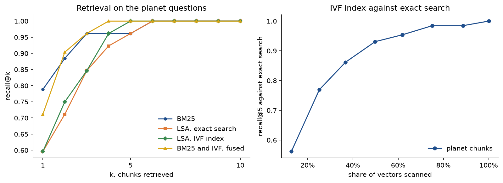
The left panel shows the same pattern as the large corpus: BM25 is best at rank 1, the fused list catches up by rank 3 and is the first to find everything, and LSA alone trails. The right panel shows the IVF trade-off on a collection small enough that exact search would always be the right choice; it is there to show the mechanism, not to save time.

The notebook retrieval_augmented_generation.ipynb is a guided tour in the order of this page: the worked example, then every stage on the corpus, the pitfalls, the grounding experiments, the bundled notes and the comparison with scikit-learn and tiktoken. The tests in tests check the worked example value by value, the mathematical properties above, the agreement with scikit-learn and, when the corpus has been downloaded, the corpus numbers quoted on this page; they run in a few seconds:

python -m pytest transformers-and-llms/retrieval-augmented-generation

Data. The corpus is ten English Wikipedia articles (Mercury, Venus, Mars, Jupiter, Saturn, Uranus, Neptune, Pluto, the Moon and Ceres), each pinned to the revision id listed in SOLAR_SYSTEM_REVISIONS: 81,296 words in 228 sections after parsing. Wikipedia text is available under the Creative Commons Attribution-ShareAlike 4.0 licence, with authorship recorded in each article's history, and the examples and notebook quote short passages under that licence. The first run downloads the rendered HTML of each revision through the MediaWiki API, about 7 MB, into .data/retrieval-augmented-generation/ at the repository root, which git ignores, pausing between requests and retrying when the API rate-limits. The revision ids fix the wikitext, but templates such as unit conversions are expanded at download time, so a much later download could format a value differently. The loader therefore compares a SHA-256 digest of each parsed article with the pinned one and warns when they differ, and a test fails if an evidence span disappears. The 64 questions and their labels are our own, the planet notes of the project and their 26 questions were written for this handbook, and the vectors of the IVF speed benchmark are synthetic and generated from a seed.

In practice

Libraries agree with the from-scratch versions

scikit-learn's TfidfVectorizer, given the package's analyze as its analyzer, produces the same tf-idf scores on the corpus, with a largest difference of 1.1 × 10⁻¹⁶ over all questions. TruncatedSVD with the ARPACK solver gives the same singular values to within 4.4 × 10⁻¹⁵ and the same chunk coordinates up to sign to within 1.4 × 10⁻¹³, and sklearn.metrics.ndcg_score the same nDCG@10 to within 3.9 × 10⁻¹⁶. BM25 is the default similarity of Lucene, and therefore of Elasticsearch and OpenSearch, with k1 = 1.2, b = 0.75 and the same positive idf; Pyserini wraps it for research use. For vectors, FAISS provides exact search (IndexFlatIP), IVF (IndexIVFFlat, and IndexIVFPQ with compressed vectors) and graph indexes (IndexHNSWFlat), and vector databases build on the same structures. tiktoken counts real model tokens: the five-source prompt for "Who discovered Triton?" has 576 word and punctuation tokens and 640 cl100k_base tokens, so the simple count used for the prompt budget runs about a tenth low.

Measured on 64 questions

On sentence chunks of at most 100 words, each indexed with its article title and section heading:

• BM25 reaches recall 0.523 at rank 1, 0.719 at 3, 0.828 at 5 and 0.883 at 10, with MRR 0.672 and nDCG@10 0.675.
• Sublinear tf-idf reaches 0.469, 0.688, 0.781 and 0.859, with MRR 0.620 and nDCG@10 0.625.
• LSA with 128 dimensions reaches 0.445, 0.625, 0.703 and 0.805, with MRR 0.568 and nDCG@10 0.577.
• BM25 and LSA fused by rank reach 0.555, 0.742, 0.766 and 0.891, with MRR 0.674 and nDCG@10 0.689.

BM25 is the strongest single retriever, as it usually is on factual questions that reuse the document's words. LSA trails it overall but wins where the wording differs ("Who discovered Uranus?" moves the evidence from rank 36 to rank 9) and loses badly where one distinctive word identifies the chunk. LSA improves from 32 to 128 dimensions (recall at 5 from 0.508 to 0.703) and gains little beyond. Fusion improves recall at 1, 3 and 10, the MRR and nDCG, and loses at 5, where some evidence that BM25 alone ranked in its top five falls just below fifth place once LSA's choices are mixed in; across questions it moves the first relevant chunk up for 16 and down for 13. With a stronger dense retriever the gain from fusion is usually larger.

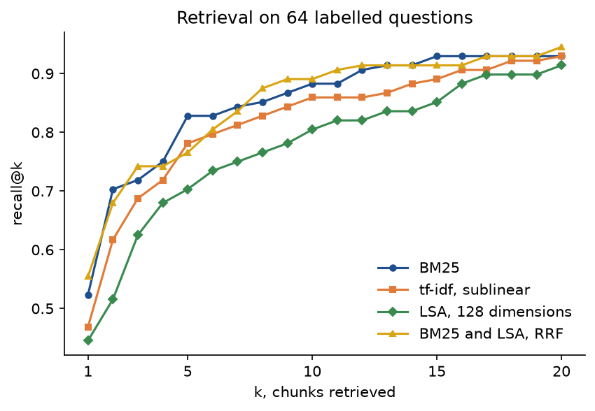
The curves cross: which retriever is best depends on how many chunks the prompt can hold. At k = 20 the fused list reaches 0.945, BM25 and tf-idf 0.930 and LSA 0.914.

Chunking matters as much as the retriever. The next figure plots recall at k for k = 1 to 10 against the number of words those k chunks put into the prompt. Sentence chunks beat fixed windows of the same size, because their borders follow the text and their headers name the right section: 100-word windows without overlap cut 3 pieces of evidence in two and reach recall 0.648 at rank 5, against 0.703 with an overlap of 25 and 0.828 for sentence chunks of up to 100 words. Whole sections reach recall 0.984 at rank 10, but their top five already cost about 2,000 words.

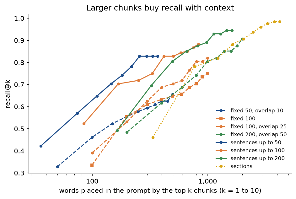
The best strategy is the one whose curve lies furthest up and to the left at the prompt size you can afford; here that is sentence chunks of 50 to 100 words.

On the 1,014 LSA vectors an IVF index with 16 lists returns 75 % of the exact top ten when it scans one list (7.3 % of the vectors) and 94 % when it scans four, while the labelled recall at 5 barely moves (0.70 to 0.73): the neighbours it misses are mostly not the relevant chunks. At this size exact search takes microseconds and an approximate index is pointless. On 100,000 synthetic vectors in 64 dimensions with 256 lists, probing 8 lists scans 3.1 % of the vectors and finds 77 % of the true neighbours in well under a tenth of the time of exact search, and probing 64 lists finds 96 % but saves much less time, because this NumPy implementation gathers the scanned vectors list by list; timings on a shared machine vary from run to run. How fast recall rises depends strongly on how clustered the vectors are.

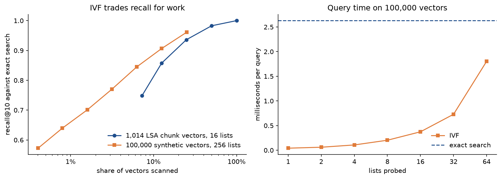
The left panel shows that both indexes find most neighbours while scanning a small share of the vectors, and that the clustered synthetic vectors need a smaller share than the LSA vectors; the right panel shows where the speed comes from and how it shrinks as more lists are probed.

The extractive generator, reading the top five chunks of the 60 single-article questions, quotes the labelled evidence for 34 of them (0.567) with either BM25 or fusion, against a retrieval ceiling of 0.828 at rank 5: once the evidence is in the prompt, picking the right sentence is the weaker step. A capable language model reads far better than coverage scoring, which is the point of putting one at the end of the pipeline.

What pretrained sentence embedders add

LSA is fitted to this collection alone, so it knows only which words co-occur in 81,000 words about planets. A pretrained sentence embedder, a transformer encoder trained contrastively on hundreds of millions of question and passage pairs and paraphrases, brings knowledge from outside the collection: it maps "How long is a year on Venus?" close to "completes an orbit every 224.7 days" and "How old is Ceres?" close to "formed 4.56 billion years ago", two of the questions that every retriever here ranks worst. It also handles questions in other languages and needs no refitting when documents are added. The costs are an encoder forward pass for every chunk at indexing time and for every question at query time, a maximum input length (often 256 to 512 tokens) that caps the chunk size, and weaker matching of exact identifiers, rare names and numbers, which is why production systems still fuse a dense retriever with BM25. A cross-encoder reranker, which reads the question and each candidate chunk together, is the usual next step after fusion. The sentence-transformers package provides such encoders in a few lines; it is not part of this repository's dependency groups, so the code here stays with LSA.

A hosted model in place of the extractive generator

Any function from a Prompt to text is a generator. hosted_generator posts the prompt to a chat-completions endpoint, the request format that many hosted services and local inference servers accept, and returns the reply, which then goes through exactly the same citation check:

import os

from retrieval_augmented_generation import answer_question, build_bench, hosted_generator

bench = build_bench()
generate = hosted_generator(
    os.environ["LLM_BASE_URL"], os.environ["LLM_API_KEY"], os.environ["LLM_MODEL"]
)
result = answer_question("Who discovered Triton?", bench.chunks, bench.hybrid(), generate, k=5)
print(result.answer)
print([(check.sentence, check.supported) for check in result.checks])

Keep the key in the environment, never in code or a notebook. Set the temperature to zero for reproducible answers, keep the instruction to cite every sentence, and check the citations anyway: models follow the format far more reliably than they follow the sources.

Retrieval without embeddings: summaries as context

A small collection can skip search altogether: write a summary of every document once, put all the summaries into the prompt, and let the model find the answer. Encyclopedia lead sections are such summaries. For the ten articles they total 4,780 words and 5,985 prompt tokens, about 600 tokens per article, so a context window of 128,000 tokens would hold roughly 213 of them. The approach works when questions concern what the summaries state: a document's subject, its main facts, which document covers what. It breaks in three ways, all measurable here. Details are missing: the evidence of only 11 of the 60 single-article questions lies in a summary, and the extractive generator answers only 6 correctly from the summaries, against 34 from five retrieved chunks. The cost grows with the collection, linearly and on every question, until the summaries no longer fit at all. And a summary written before the questions are known cannot anticipate them. Summaries still make a good first stage: searching the ten summaries with BM25 picks the right article for 41 of the 60 questions, after which chunks can be searched within that article only.

When to use which

• Start with BM25 over sentence-sized chunks with title and heading headers. It needs no model, explains its scores, and is hard to beat on questions that reuse the documents' words.
• Add a dense retriever when questions paraphrase the documents, and fuse it with BM25 by rank; measure the fusion on your own labelled questions, because it can lose at some depths, as it does here at k = 5.
• Choose the chunk size by recall per prompt token, not recall alone. Overlap fixed windows by at least the length of a typical answer span, or better, chunk on sentence and section boundaries.
• Use exact search up to around a hundred thousand vectors; beyond that use IVF or a graph index such as HNSW and tune the number of probes on labelled questions, not only on recall against exact search.
• Put summaries of every document into the prompt only for small collections and gist questions; use them to route questions in larger ones.

Pitfalls

• Chunks that lose their subject. "Radar observations in 1965 proved that the planet has a 3:2 spin-orbit resonance" never says Mercury. With 30-word sentence chunks, 8 pieces of evidence sit in chunks that never name their body, and indexing the text without its title and heading lowers recall at 5 from 0.672 to 0.594. With 100-word chunks the header still raises recall at 5 from 0.781 to 0.828, although recall at 1 drops slightly, from 0.555 to 0.523. examples/chunking_strategies.py prints both.
• Fixed windows that cut the evidence. A window without overlap cuts a span of L words with probability (L - 1)/W, and no ranking can recover a cut span; an overlap of at least L - 1 words removes the problem. 100-word windows cut 3 of the 68 pieces of evidence here and an overlap of 25 cuts none, as examples/chunking_strategies.py shows with the solar day of Mars split between two windows.
• The classic BM25 idf goes negative. The Robertson and Spärck Jones weight is negative when a term is in more than half the chunks. On the worked example it gives moons the weight 0 and mars -0.8473, so the chunk about Jupiter, which does not mention Mars, ranks first, as examples/worked_example.py prints and tests/test_worked_example.py asserts. Use the version with the added one.
• Raw dot products favour long chunks. Without the division by the vector lengths, tf-idf on section chunks drops from recall 0.820 at rank 5 to 0.672, and the mean length of the top five sections rises from 419 to 653 words against 357 over all sections (examples/compare_retrievers.py).
• Fusing raw scores. BM25 scores here reach 26.0 and LSA cosines 0.93, so their sum returns exactly BM25's top five for 62.5 % of the questions; the effective weight is an accident of scale that changes with query length. Fuse ranks, or normalize each score list and tune the weight on labelled questions.
• Tuning an approximate index against exact search only. Recall against exact search rises from 0.748 to 1.000 as more lists are probed, while the labelled recall at 5 stays between 0.70 and 0.73. Synthetic benchmarks flatter IVF too: with tightly clustered vectors one probe finds almost every neighbour, with diffuse ones far fewer, so tune on vectors and questions from your own collection (examples/vector_search.py).
• A confident answer that the sources do not support. A trigram model trained on the corpus, standing in for a generator that answers from memory, completes "A day on Pluto lasts" with "about 176 Earth days.", fluently and with a geometric-mean token probability of 0.388. 176 Earth days is Mercury's solar day. The five chunks retrieved for "What is the rotation period of Pluto?" contain the true value, 6.387 Earth days, and the support check flags 176 as a number found in none of them. The model's own probability is no guide: from memory it prefers 176 over 6.387 by three to one, while conditioned on the retrieved chunks it prefers 6.387 by about four to five orders of magnitude. Both parts of the check fire here: only 0.67 of the claim's terms occur in the sources, below the 0.75 threshold, and 176 occurs nowhere. The number check matters most when the words do match; in tests/test_trigram.py an invented number sits in a claim with 0.8 overlap and only the number check catches it (examples/grounded_answers.py).
• RAG-Token can swap facts between sources. For "Which has more known moons, Saturn or Jupiter?", RAG-Token gives the correct sentence a likelihood about 800 times higher than RAG-Sequence does, because each number can come from a different chunk, but it also gives the sentence with the two numbers swapped about half the likelihood of the correct one, because nothing ties a number to the chunk that names its planet (examples/grounded_answers.py).
• A citation is not an answer. The corpus says that Pioneer 11 measured the temperature of Titan but never gives the value. Asked "What is the surface temperature of Titan?", the extractive generator quotes exactly that sentence with coverage 0.83, cites the right source, and passes the citation check with full support; the answer contains no temperature. Faithfulness to the sources and relevance to the question are separate checks, and only the first is automated here.
• Coverage or token probability as confidence. Raising the abstention threshold to 0.5 refuses 3 of the 4 questions the corpus cannot answer, but not the Titan question, while the number of answered questions falls from 60 to 48 and the correct ones from 34 to 30; higher thresholds lose more correct answers and refuse nothing more. The sample project shows the same trade-off on the planet notes, where the threshold of 0.5 refuses every unanswerable question but also 8 of the 25 answerable ones. A confident wrong answer and a confident right one look alike to these scores, as the 0.388 token probability of the Pluto answer shows.
• The corpus disagrees with itself. Neptune's lead gives an orbital period of 164.8 years and winds of 580 m/s; its body gives 164.79 years and almost 600 m/s. A question labelled against one sentence marks the other wrong, so labels must list every span that states a fact, as the question set here does (examples/grounded_answers.py).
• Computing the ideal DCG from the retrieved list. The ideal must come from every relevant chunk in the collection. With one of two relevant chunks retrieved, at rank 3, the honest nDCG@3 is 0.3066; dividing by the ideal of the retrieved list alone gives 0.5 and rewards the retriever for missing the other chunk (tests/test_metrics.py).

Further reading

• P. Lewis, E. Perez, A. Piktus et al., "Retrieval-augmented generation for knowledge-intensive NLP tasks", NeurIPS 2020. The RAG-Sequence and RAG-Token models.
• K. Guu, K. Lee, Z. Tung, P. Pasupat and M.-W. Chang, "REALM: retrieval-augmented language model pre-training", ICML 2020.
• S. Robertson and H. Zaragoza, "The probabilistic relevance framework: BM25 and beyond", Foundations and Trends in Information Retrieval 3(4), 333-389, 2009.
• S. E. Robertson and K. Spärck Jones, "Relevance weighting of search terms", Journal of the American Society for Information Science 27(3), 129-146, 1976.
• S. Deerwester, S. T. Dumais, G. W. Furnas, T. K. Landauer and R. Harshman, "Indexing by latent semantic analysis", Journal of the American Society for Information Science 41(6), 391-407, 1990.
• C. D. Manning, P. Raghavan and H. Schütze, Introduction to Information Retrieval, Cambridge University Press, 2008. Chapters 6, 8, 11 and 18 cover tf-idf, evaluation, probabilistic retrieval and LSA.
• G. V. Cormack, C. L. A. Clarke and S. Büttcher, "Reciprocal rank fusion outperforms Condorcet and individual rank learning methods", SIGIR 2009.
• H. Jégou, M. Douze and C. Schmid, "Product quantization for nearest neighbor search", IEEE Transactions on Pattern Analysis and Machine Intelligence 33(1), 117-128, 2011. The IVF index with compressed vectors.
• Y. A. Malkov and D. A. Yashunin, "Efficient and robust approximate nearest neighbor search using hierarchical navigable small world graphs", IEEE Transactions on Pattern Analysis and Machine Intelligence 42(4), 824-836, 2020.
• V. Karpukhin, B. Oğuz, S. Min et al., "Dense passage retrieval for open-domain question answering", EMNLP 2020.
• N. Reimers and I. Gurevych, "Sentence-BERT: sentence embeddings using Siamese BERT-networks", EMNLP 2019.
• N. Thakur, N. Reimers, A. Rücklé, A. Srivastava and I. Gurevych, "BEIR: a heterogeneous benchmark for zero-shot evaluation of information retrieval models", NeurIPS Datasets and Benchmarks 2021. BM25 remains a strong baseline across domains.
• K. Järvelin and J. Kekäläinen, "Cumulated gain-based evaluation of IR techniques", ACM Transactions on Information Systems 20(4), 422-446, 2002.
• N. F. Liu, K. Lin, J. Hewitt et al., "Lost in the middle: how language models use long contexts", Transactions of the Association for Computational Linguistics 12, 157-173, 2024.
• S. Es, J. James, L. Espinosa-Anke and S. Schockaert, "RAGAS: automated evaluation of retrieval augmented generation", EACL 2024 system demonstrations. Faithfulness and answer-relevance measures with a language model as judge.

Related topics: N-gram language models for the trigram generator, Text representations for tf-idf and word vectors, Dimensionality reduction for the SVD behind LSA, Clustering for k-means, Search engines for inverted indexes at scale, Decoding strategies for beam search, and Prompting and structured output for prompt design.