Perceptrons and multilayer networks¶

Every neural network is built from one simple part: a unit that forms a weighted sum of its inputs and passes it through an activation function. With a hard threshold as the activation, one such unit already computes logic gates, and a short learning rule finds its weights from examples whenever a straight line can separate the classes. It cannot compute XOR, and the reason, together with the fix, explains what the hidden layers of every larger network are for. This page builds the perceptron as a linear threshold unit, runs its learning rule by hand and proves that it converges, shows how one hidden layer makes XOR separable, replaces the threshold by the sigmoid so that gradients exist, writes the forward pass of a multilayer network in matrix form, and measures two things the theory promises: one hidden layer approximates any continuous function as it widens, and depth buys what width pays for exponentially. A sample project on two interleaved spirals closes the loop. Afterwards you will be able to design small threshold networks by hand, carry out and bound the perceptron rule, state the universal approximation theorem without overstating it, and reason about what each hidden unit of a trained network computes.

To run the code in this topic, install the base group, the ml group for the linear programs and the scikit-learn comparisons, and the deep group for the comparison with PyTorch.

Intuition¶

A biological neuron collects electrical signals from thousands of other cells and, when their combined effect crosses a threshold, fires a pulse along its axon to the cells it connects to. The artificial unit keeps only that outline, a weighted sum compared with a threshold, and everything below follows from the mathematics of the abstraction rather than from biology.

A threshold unit: inputs x1, x2 up to xn and a constant input 1 feed a weighted sum through the weights w1 to wn and the bias b, the sum z goes into a threshold that outputs 1 when z is positive and 0 otherwise, and that is the output

The diagram shows the whole unit. The constant input 1 carries the bias, which shifts the threshold away from zero. The inputs with a weighted sum of exactly zero form a line in the plane, a plane in three dimensions and a hyperplane in general, so the unit answers one question: on which side of its line does the input lie? AND, OR and NOT are such questions for suitably placed lines.

Learning means moving the line. The perceptron rule looks at one example at a time and, whenever the example lies on the wrong side, tilts and shifts the line towards it. If some line separates the classes with room to spare, the rule finds a separating line after a bounded number of corrections, and the bound depends only on how much room there is.

XOR has no such line: its two classes sit on the two diagonals of the unit square, and the diagonals cross. The fix is to compute new features first. Two hidden units each draw a line, one answering "is at least one input on?" and the other "is at most one input on?", and in the space of their answers the classes are separable, so a third unit finishes the job.

The XOR network: inputs x1 and x2 feed hidden unit 1, an OR gate with bias -1, through weights 2 and 2, and hidden unit 2, a NAND gate with bias 3, through weights -2 and -2; both hidden units feed the output unit, an AND gate with bias -3, through weights 2 and 2

The weights are written on the edges and the biases inside the units. That is what hidden units do in general: they redescribe the input until the output layer's linear decision becomes possible.

To learn hidden layers by gradient descent the hard threshold has to go, because its slope is zero everywhere it exists. The sigmoid is a smoothed threshold with a usable derivative, and with it a network is a differentiable function of its weights that backpropagation can train. Two theorems then describe what such networks can represent: one hidden layer approximates any continuous function on a bounded region if it is wide enough, and some functions need exponentially fewer units when the same budget is spent on depth.

How it works¶

Notation¶

The layer notation is the one used throughout this part. Vectors are columns, and for a single unit:

x is one input with n components, y in {0, 1} its class and t = 2y - 1 in {-1, +1} the signed label the learning rule uses.
w holds the weights and b the bias of the unit, z is its net input and ŷ its output.
H is the step, or Heaviside, function, which is 1 for positive arguments and 0 otherwise.
x̃ = (x, 1) and w̃ = (w, b) are the augmented input and weights, which fold the bias into the weights.
η > 0 is the learning rate, and R, γ and u are the radius, margin and unit-length separator of the convergence theorem.

For a network, layer 0 is the input and layer l has n units, for l from 1 to L. The weight matrix W of layer l has one row per unit of layer l and one column per unit of layer l - 1, so its entry in row j and column k is the weight to unit j from unit k, the layout of torch.nn.Linear.weight. The bias vector b, the activation function f, the net inputs z and the activations a of layer l follow, with the input x as the activations of layer 0. In a mini-batch with one example per row, X holds the inputs and Z and A the net inputs and activations of a layer. The formula images write the layer as a superscript in parentheses. In the text, W1, b1, Z1 and A1 are short for the weights, biases, net inputs and activations of layer 1, and likewise for layer 2.

The perceptron: a linear threshold unit¶

A perceptron computes a weighted sum of its inputs plus a bias, and outputs 1 when the sum is positive:

The net input z is w transposed x plus b, the sum over k of w k times x k plus b, and the output is H of z; H of z is 1 for z greater than 0 and 0 for z less than or equal to 0

The decision boundary, the inputs with z = 0, is a hyperplane with normal vector w. In two dimensions with w2 ≠ 0 it is the line

x2 equals minus w1 over w2 times x1 minus b over w2

and the signed distance from a point to it is

The signed distance d of x is w transposed x plus b, divided by the length of w

which is positive on the side w points to, where the unit outputs 1. Multiplying w and b by any c > 0 multiplies z by c and leaves every output unchanged, so a threshold unit has no preferred scale; the scale starts to matter once the threshold is replaced by a sigmoid. The bias shifts the boundary away from the origin, and it is convenient to treat it as the weight of an extra input that is always 1:

The augmented input x tilde is x with a 1 appended, the augmented weights w tilde are w with b appended, and z equals w tilde transposed times x tilde

Some texts write a threshold θ = -b and fire when the weighted sum is at least θ. The difference between "greater than" and "at least" matters only for points exactly on the boundary, but it does matter there, as the learning rule below shows.

Logic gates as perceptrons¶

With inputs in {0, 1}, a gate is a perceptron whose four net inputs have the right signs. For AND the conditions are, one per row of the truth table,

AND requires b at most 0, w2 plus b at most 0, w1 plus b at most 0, and w1 plus w2 plus b greater than 0

Any equal weights w > 0 with w ≤ -b < 2w satisfy them. This page uses weights (2, 2) and bias -3, which puts every net input at ±1 or ±3 and the boundary on the line x1 + x2 = 1.5. OR needs b ≤ 0 < w1 + b and w2 + b, met by weights (2, 2) and bias -1. NAND is AND with every sign flipped, weights (-2, -2) and bias 3: the same line with the sides swapped. NOT has one input and needs b > 0 ≥ w + b, met by w = -2 and b = 1.

NAND alone suffices to build every Boolean circuit, so networks of threshold units compute every Boolean function. A single hidden layer is already enough: give each input pattern with output 1 its own hidden unit that fires for exactly that pattern, and let the output unit compute the OR of the hidden units. For n inputs that can take up to 2ⁿ hidden units, the Boolean counterpart of the width the universal approximation theorem below may need.

The perceptron learning rule¶

Given examples xᵢ with labels yᵢ, start from w̃ = 0 and visit the examples in turn. Call example i a mistake when it lies on the wrong side or exactly on the boundary, and on a mistake add the signed example to the weights:

The signed label t i is 2 y i minus 1, and example i is a mistake exactly when t i times w tilde transposed x tilde i is at most 0; the update adds eta t i x tilde i to w tilde, that is eta t i x i to w and eta t i to b

A pass over all examples is an epoch; the rule stops after an epoch without a mistake. The update moves the boundary in the right direction for the example that caused it. Since t² = 1, the new value of t z for that example is

t i times the updated weights transposed x tilde i equals t i w tilde transposed x tilde i plus eta times the squared length of x tilde i

so t z grows by η times the squared length of x̃, though it need not turn positive yet, and other examples may get worse.

The rule is often written with the error y - ŷ in place of t:

w tilde becomes w tilde plus eta times y i minus y hat i times x tilde i, where y hat i is H of w tilde transposed x tilde i

On a mistake y - ŷ equals t, so the two forms agree except for a class-0 example with z = 0 exactly, which the y - ŷ form leaves alone because H(0) = 0. The form with t z ≤ 0 is the one the convergence proof uses and the one scikit-learn implements. It is also stochastic subgradient descent on the perceptron criterion

The perceptron criterion E i of w tilde is the maximum of 0 and minus t i w tilde transposed x tilde i

taking -t x̃ as its subgradient when t z ≤ 0 and 0 otherwise. Starting from zero, the weights after any sequence of updates are η times a sum of the vectors t x̃, and which updates happen depends only on signs. Every run with learning rate η is therefore the run with η = 1 scaled by η, with the same predictions at every step: for the perceptron rule from a zero start, the learning rate does nothing.

The perceptron convergence theorem¶

The theorem says that a margin guarantees convergence. Suppose some unit vector u puts every augmented example on its correct side with room γ to spare, and let R be the length of the longest augmented example:

If u has length 1, t i u transposed x tilde i is at least gamma greater than 0 for every i, and R is the largest length of x tilde i, then the number of updates is at most R over gamma squared

Then the perceptron rule started from zero makes at most (R / γ)² updates, for any learning rate and any order of visiting the examples. The proof follows the weights w̃ after the k-th update, made on some example i, with two estimates that pull in opposite directions. First, the weights gain on u at a steady rate, because every update adds at least η γ to their projection on u:

u transposed w tilde k equals u transposed w tilde k minus 1 plus eta t i u transposed x tilde i, which is at least u transposed w tilde k minus 1 plus eta gamma; by induction u transposed w tilde k is at least k eta gamma

Second, their length grows slowly, because the middle term below is not positive on a mistake:

The squared length of w tilde k equals the squared length of w tilde k minus 1 plus 2 eta t i w tilde k minus 1 transposed x tilde i plus eta squared times the squared length of x tilde i, which is at most the squared length of w tilde k minus 1 plus eta squared R squared; by induction it is at most k eta squared R squared

A projection on a unit vector can never exceed the length of the vector, by the Cauchy-Schwarz inequality, so the two estimates squeeze k:

k eta gamma is at most u transposed w tilde k, which is at most the length of w tilde k, which is at most the square root of k times eta R; therefore k is at most R over gamma squared

The projection grows linearly in k while the length grows only like the square root of k, and that cannot go on forever. A few remarks make the statement usable:

Any separator gives a bound, and the best one uses the largest margin, the maximum-margin separator through the origin of the augmented space:

gamma star is the maximum over unit vectors u of the minimum over i of t i u transposed x tilde i

This is a close relative of the problem support vector machines solve, which leave the bias out of the norm. A finite dataset that is linearly separable at all has γ* > 0. - R and γ belong to the augmented vectors. Moving the whole dataset far from the origin does not change whether it is separable, but it inflates R and shrinks the augmented margin, so the bound grows; centring the inputs first is cheap insurance. - The theorem bounds updates, not epochs. Every epoch before the last makes at least one update, so there are at most (R / γ)² + 1 epochs. - Without separability there is no convergence. The weights stay bounded, by the perceptron cycling theorem of Block and Levin, but they keep changing, and the last iterate can be arbitrarily poor. The pocket algorithm keeps the best weights seen so far and the averaged perceptron returns the average of all iterates; for overlapping classes, logistic regression is usually the better tool.

Why XOR is not linearly separable¶

XOR outputs 1 for (0, 1) and (1, 0) and 0 for (0, 0) and (1, 1). Suppose a perceptron computed it. The four rows of the truth table require the first line below, and adding the last two conditions and the first two gives the same sum with opposite signs:

XOR requires b at most 0, w1 plus w2 plus b at most 0, w2 plus b greater than 0 and w1 plus b greater than 0; adding the last two gives w1 plus w2 plus 2b greater than 0, adding the first two gives w1 plus w2 plus 2b at most 0

The argument does not depend on the convention at z = 0: with "at least" in place of "greater than" the inequalities swap strictness and contradict each other the same way. Geometrically, the midpoint (0.5, 0.5) is the average of the two class-1 points and also the average of the two class-0 points. Because z is an affine function of x, its value at the midpoint is the average of its values at either pair, so it would have to be positive and not positive at once. In general two finite sets are linearly separable exactly when their convex hulls do not meet, and the hulls of the XOR classes are the two diagonals of the square, which cross. The same holds for the parity of n ≥ 2 bits. Minsky and Papert made this limitation of single-layer perceptrons famous in 1969, at a time when nobody knew how to train the hidden layers that remove it.

A two-layer network for XOR¶

XOR is "at least one, but not both":

XOR of x1 and x2 equals AND of OR of x1 and x2 and NAND of x1 and x2

Each of the three gates is a perceptron from above, so XOR is computed by a network with two layers of step units: W1 has the rows (2, 2) and (-2, -2) and b1 = (-1, 3), so hidden unit 1 is the OR gate and hidden unit 2 the NAND gate, and the output layer has W2 = (2, 2) and b2 = -3, the AND gate. The hidden layer maps the four inputs to

The hidden layer maps (0, 0) to (0, 1), (0, 1) to (1, 1), (1, 0) to (1, 1) and (1, 1) to (1, 0)

In this hidden space the two class-1 inputs have merged into the single point (1, 1), and the line of the output AND gate separates it from the other two. The hidden layer has not solved the problem; it has changed the description of the inputs so that a linear unit can.

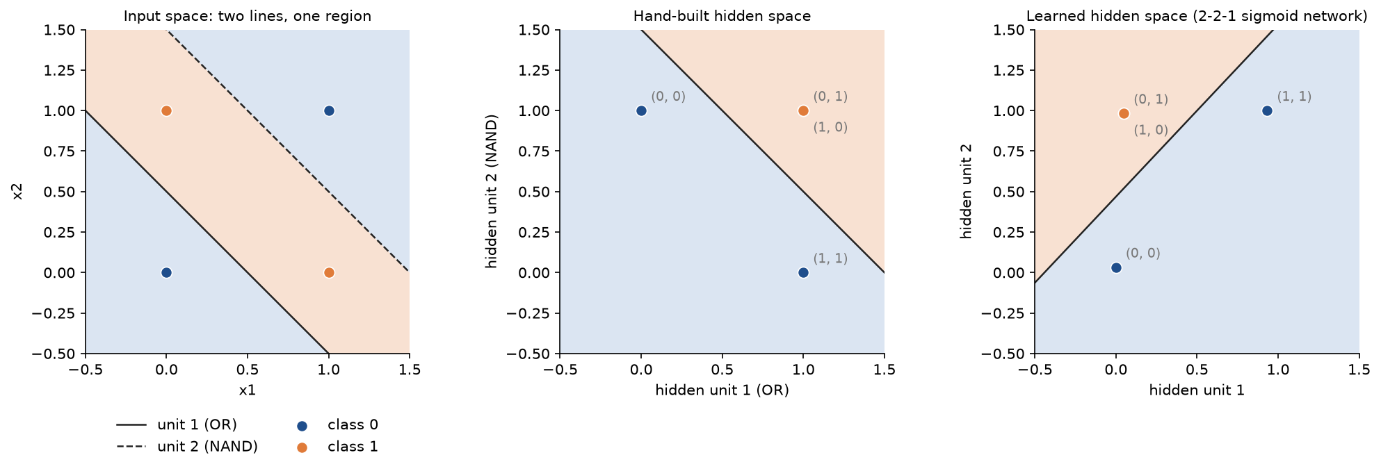
Seen from the input space, each hidden threshold unit is the indicator of a half-plane and the output unit takes a weighted vote of these indicators. Here the vote is an intersection, so the class-1 region is the strip between the two parallel lines x1 + x2 = 0.5 and x1 + x2 = 1.5. A single hidden layer of threshold units can form any intersection of half-planes, which is a convex region; a second hidden layer can take unions of such regions. A network trained by gradient descent need not find this decomposition: in the right panel, a 2-2-1 sigmoid network has learned a soft AND and a soft OR and outputs "OR and not AND".

Sigmoid neurons and why smooth activations are needed¶

Training by gradient descent needs the derivative of the cost with respect to every weight. For a threshold unit that derivative vanishes:

The derivative of y hat with respect to w k is H prime of z times x k, which is 0 for every z other than 0

Any cost computed from the outputs is therefore piecewise constant in the weights. A small change of a weight either changes no output or flips one, and the gradient is zero almost everywhere. The perceptron rule escapes this by not using gradients, but it needs a target for the unit it corrects, and a hidden unit has none: whether it should have fired is not written in the data. This is the credit assignment problem, and it is why hidden layers of threshold units were not trainable. The sigmoid replaces the step by a smooth curve with the same limits:

The sigmoid of z is 1 over 1 plus e to the minus z, and its derivative is sigma of z times 1 minus sigma of z, which is at most one quarter

A sigmoid neuron outputs a = σ(w x + b), and to first order a small change of the parameters changes the output by a small amount:

The change in a is approximately sigma prime of z times the sum over k of x k times the change in w k, plus the change in b

The cost becomes a differentiable function of every weight in the network, and backpropagation computes all its derivatives. Nothing is lost by the switch, because steeper and steeper sigmoids approach the step:

sigma of c z tends to H of z as c tends to infinity, for every z other than 0

Multiplying all weights and biases of a threshold network by a large c and replacing each step by a sigmoid therefore gives a smooth network that computes nearly the same function; the worked example does this for XOR.

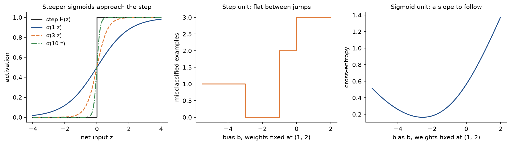
The middle panel is what a threshold unit can measure as its bias moves: flat stretches give no hint which way to go. The right panel is the same unit with a sigmoid output, whose cost has a slope everywhere. A sigmoid output can also be read as a probability, which is the link to logistic regression, a single sigmoid neuron trained with the cross-entropy cost. Modern hidden layers mostly use tanh z = 2σ(2z) - 1 or the rectified linear unit ReLU(z) = max(0, z), which is differentiable except at 0; Activations and initialization compares them.

The forward pass in matrix form¶

A multilayer perceptron, or fully connected feedforward network, applies one layer after another:

The net inputs of layer l are W of layer l times the activations of layer l minus 1 plus b of layer l, the activations of layer l are f l of the net inputs, and the activations of layer 0 are the input x

Entry j of the matrix product is the weighted sum over the units feeding unit j:

The net input of unit j in layer l is the sum over k of the weight to j from k times the activation of unit k in layer l minus 1, plus the bias of unit j

The name is historical: the units are usually sigmoid, tanh or ReLU units, not threshold units. For a mini-batch with one example per row, transposing each equation gives one row of a matrix equation, and the whole batch takes one matrix product per layer:

For a batch, A0 is X, the net inputs of layer l are the activations of layer l minus 1 times the transposed weights plus a column of ones times the transposed biases, and the activations are f l applied to the net inputs

The bold 1 is a column of ones, one per example, so that the bias is added to every row.

The forward pass of a two-layer network for a batch of m examples: the batch X, m rows by n0 columns, times W1 transposed plus b1 on every row gives the net inputs Z1, m by n1; f1 applied entry by entry gives the activations A1; times W2 transposed plus b2 gives Z2, m by n2, and f2 gives the outputs A2

The diagram follows the shapes through two layers; W1 is n1 by n0, so the product of the batch with its transpose has one row per example and one column per unit. Each layer has one weight per incoming unit and one bias for each of its units:

The number of parameters of layer l is n l times n l minus 1 plus 1

The output activation follows the task: a sigmoid for two classes, the identity for regression, and for several classes the softmax

Output j of the softmax is e to the z j divided by the sum over i of e to the z i

The activations must be nonlinear. If every f is the identity, substituting each layer into the next leaves a single affine map however many layers there are:

Such a network cannot compute XOR; the best affine fit to XOR in the least-squares sense is the constant 0.5.

The universal approximation theorem¶

The theorem is due to Cybenko (1989) for sigmoidal activations and to Hornik, Stinchcombe and White (1989), with the form below by Leshno, Lin, Pinkus and Schocken (1993). Let f be continuous and not a polynomial, let K be a compact set of inputs, and let g be continuous on K. Then for every ε > 0 there are a width N and parameters of a network with one hidden layer and a linear output,

F of x equals W2 times f1 of W1 x plus b1, plus b2, which is the sum over j from 1 to N of the output weight of unit j times f1 of the sum over k of W1 j k x k plus b1 j, plus b2

such that the network is uniformly close to g:

The absolute difference between g of x and F of x is less than epsilon for every x in K

Sigmoid, tanh and ReLU all qualify, the step is allowed too, and vector-valued targets are handled one output at a time. A polynomial activation of degree d fails, because then F is a polynomial of degree at most d whatever N is; the identity is the extreme case of the collapse above.

In one dimension the proof idea fits in two constructions, both implemented in approximation.py. Take N equal intervals on K = [α, β] with knots

The spacing h is beta minus alpha over N, and the knots are x j equals alpha plus j h for j from 0 to N

The first construction is a ReLU network that interpolates linearly. With the slope s of g on each interval, every hidden unit switches on at one knot and changes the slope by the right amount:

s j is g of x j minus g of x j minus 1, over h; F of x is g of x0 plus s1 ReLU of x minus x0 plus the sum over j from 1 to N minus 1 of s j plus 1 minus s j times ReLU of x minus x j

On the interval that ends at knot j the slopes add up to the slope of g on that interval, and F starts at g at the first knot, so F is the broken line through the values of g at all the knots. It is a network with N hidden units: W1 is a column of ones, the hidden biases are minus the knots, the output weights are the slope changes and the output bias is the value of g at the first knot. For twice differentiable g the error of linear interpolation is

The absolute difference between g of x and F of x is at most h squared over 8 times the largest absolute second derivative of g

so the error falls like 1/N². The second construction is a sigmoid network that climbs a soft staircase, one soft step of the right height in the middle of every interval, with steepness c / h:

m j is the midpoint of the interval, k is c over h; F of x is g of x0 plus the sum over j from 1 to N of g of x j minus g of x j minus 1, times sigma of k times x minus m j

With exact steps in place of the sigmoids, F equals the value of g at a knot all the way between the neighbouring midpoints, within L h / 2 of g when L is the largest slope of g. Each sigmoid differs from its step by a tail that shrinks exponentially with the distance from its midpoint, and since the midpoints are h apart these tails form two geometric series. With σ(-s) ≤ e⁻ˢ the total error is at most

The absolute difference between g of x and F of x is at most L h times 1 plus 1 over e to the c minus 1 plus e to the minus c over 2 over 1 minus e to the minus c, where L is the largest absolute slope of g

which is about 1.007 L h for c = 10: the error falls like 1/N.

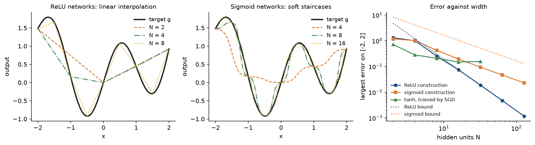
The figure, from examples/universal_approximation.py, uses the target g(x) = sin 3x + 0.3 x² on [-2, 2]. Both constructions follow their predicted rates, the ReLU one sitting on its bound from N = 32 on, while networks trained by gradient descent stop improving long before. The theorem is often quoted as "neural networks can learn any function". It says much less:

It is an existence statement. It gives no rule for the weights and says nothing about whether gradient descent finds them; the trained networks in the figure stall far above the error of the constructions.
It gives no useful bound on N. The constructions need a grid, and in n dimensions a grid of spacing h has (1/h)ⁿ cells, so for targets known only to be smooth the width can grow exponentially with the input dimension. Barron (1993) showed that the picture is better for a restricted class: if the Fourier transform of g has a finite first moment, a sigmoid network with N units reaches a mean squared error of order 1/N on a ball of radius r, whatever the dimension:

C g is the integral of the length of omega times the absolute Fourier transform of g at omega; the mean squared error is at most 2 r C g squared over N

The constant can itself grow with the dimension, so this is a statement about a class of functions, not a free lunch. - It holds on the compact set K only. Outside it nothing is promised, and a ReLU network continues linearly. - It says nothing about learning from finite, noisy data, which is a question of generalization and regularization.

Depth changes the picture too: ReLU networks of width n + 1 and unbounded depth are also universal approximators (Hanin and Sellke 2017).

Depth versus width¶

Count linear pieces. A ReLU network on a one-dimensional input computes a continuous piecewise linear function. With one hidden layer of N units,

F of x is the sum over j from 1 to N of the output weight of unit j times ReLU of W1 j 1 x plus b1 j, plus b2

can change slope only at the N breakpoints where a unit switches on, so it has at most N + 1 pieces. A deeper network can do much better. The tent map needs two ReLU units and maps [0, 1] onto itself, running up and back down:

t of x is 2 ReLU of x minus 4 ReLU of x minus one half; t of x is 2 x on the interval from 0 to one half and 2 minus 2 x on the interval from one half to 1

Composing it k times gives a sawtooth with 2ᵏ pieces: each piece of the (k - 1)-fold composition sweeps monotonically across [0, 1], and t turns that sweep into two pieces. As a network it has k hidden layers of two units, the combination 2 a1 - 4 a2 of each layer folded into the weights of the next:

The tent network: input x feeds two layer-1 units, ReLU of x and ReLU of x minus one half, through weights 1 and 1; each feeds both layer-2 units, ReLU of t of x and ReLU of t of x minus one half, through weights 2 and minus 4; k minus 2 more layers of the same kind follow, and an identity output unit computes 2 a1 minus 4 a2 of the last layer, the k-fold tent with 2 to the k pieces

Every hidden layer receives the weights 2 and -4 from the two units before it, which hands it the tent value of the layer before, and adds its own biases 0 and -1/2. That is 2k hidden units and 6k + 1 parameters. A network with one hidden layer needs at least 2ᵏ - 1 hidden units to have 2ᵏ pieces, and 3 · 2ᵏ - 2 parameters with that many units. For k = 10 the deep network has 20 hidden units and 61 parameters; one hidden layer needs at least 1,023 units and 3,070 parameters.

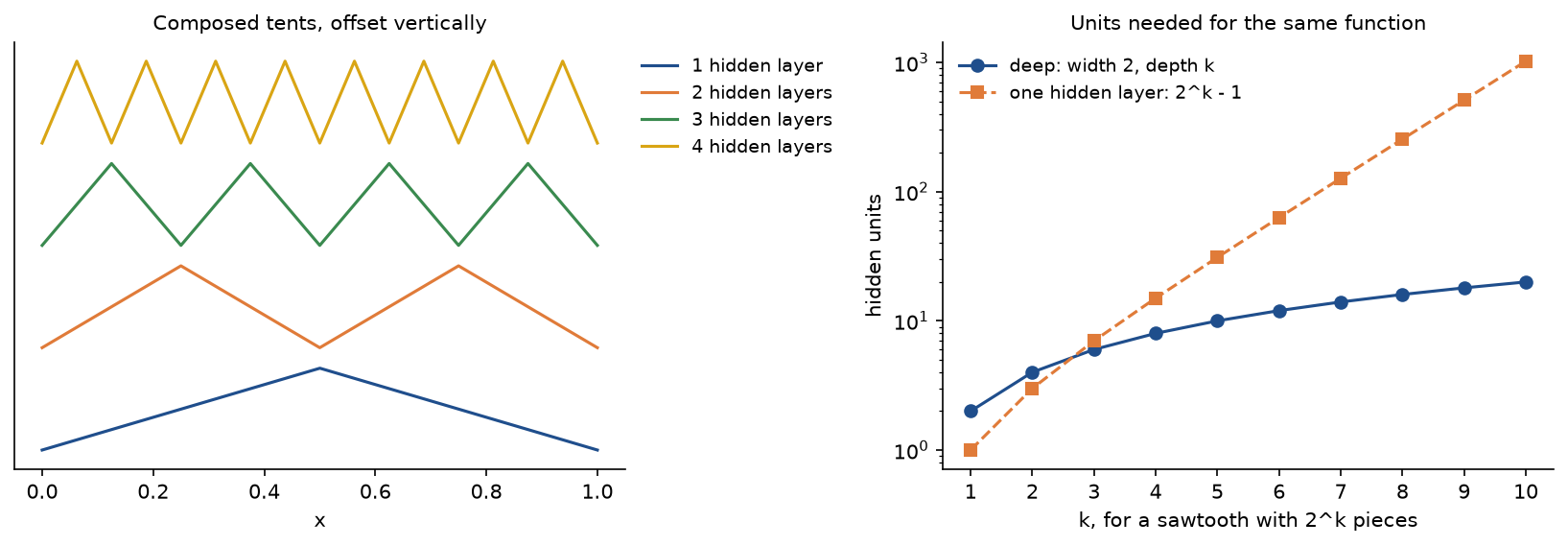
Two panels. Left, the composed tents for one to four hidden layers, offset vertically, with 2, 4, 8 and 16 linear pieces. Right, the hidden units needed for a sawtooth with 2 to the k pieces on a logarithmic axis: the deep network's 2k grows in a straight line, one hidden layer's 2 to the k minus 1 grows exponentially

From k = 3 on, the one-layer network needs more units than the deep one, and the gap then doubles with every k. The same argument bounds any depth: if layer l - 1 outputs functions with p pieces, each unit of layer l applies a ReLU to a function with p pieces and adds at most p breakpoints, so a network with hidden widths n1 to n(L-1) has at most

The number of pieces is at most the product over the hidden layers of n l plus 1

pieces. Depth multiplies, width adds. Telgarsky (2016) showed that the separation survives approximation: networks with few layers need exponentially many units even to come close to such deep sawtooth functions. Depth is not free, though. It helps for functions with repeated or compositional structure, not for every function, and deep networks are harder to train, as Backpropagation shows with vanishing and exploding errors and the sample project shows on the spirals.

Training a multilayer perceptron¶

Training minimizes the average cost over the examples by mini-batch gradient descent. Each output activation has a matching cost: the sigmoid with the binary cross-entropy, the softmax with the categorical cross-entropy and the identity with half the squared error. In each of the three pairs the output error of Backpropagation simplifies to the output minus the target,

The output error delta of layer L equals the output activations minus the target y

and the remaining backpropagation equations pass it back and turn it into gradients; this page reuses them without deriving them again. Loss functions explains why the pairing matters and Optimizers treats better update rules than plain gradient descent.

Unlike the perceptron criterion for one unit, the cost of a network with hidden layers is not convex in its weights. Gradient descent can stall in poor regions, and where it ends depends on the starting point. The weights must start random, because identical hidden units receive identical gradients and stay identical. On XOR, a 2-2-1 sigmoid network from a random start solves the problem in 39 of 50 runs; extra hidden units make bad starts rare.

Worked example¶

The examples print every number below, and the tests in tests assert the hand-calculation values one by one.

Logic gates¶

The gates with the weights chosen above give these net inputs, followed by the outputs, for the inputs (0, 0), (0, 1), (1, 0) and (1, 1) in that order:

AND, z = 2 x1 + 2 x2 - 3: net inputs -3, -1, -1 and 1, outputs 0, 0, 0 and 1.
OR, z = 2 x1 + 2 x2 - 1: net inputs -1, 1, 1 and 3, outputs 0, 1, 1 and 1.
NAND, z = -2 x1 - 2 x2 + 3: net inputs 3, 1, 1 and -1, outputs 1, 1, 1 and 0.
NOT, z = -2 x + 1: net input 1 and output 1 for x = 0, net input -1 and output 0 for x = 1.

The decision lines are x2 = -x1 + 1.5 for AND and NAND and x2 = -x1 + 0.5 for OR, and NOT switches at x = 0.5.

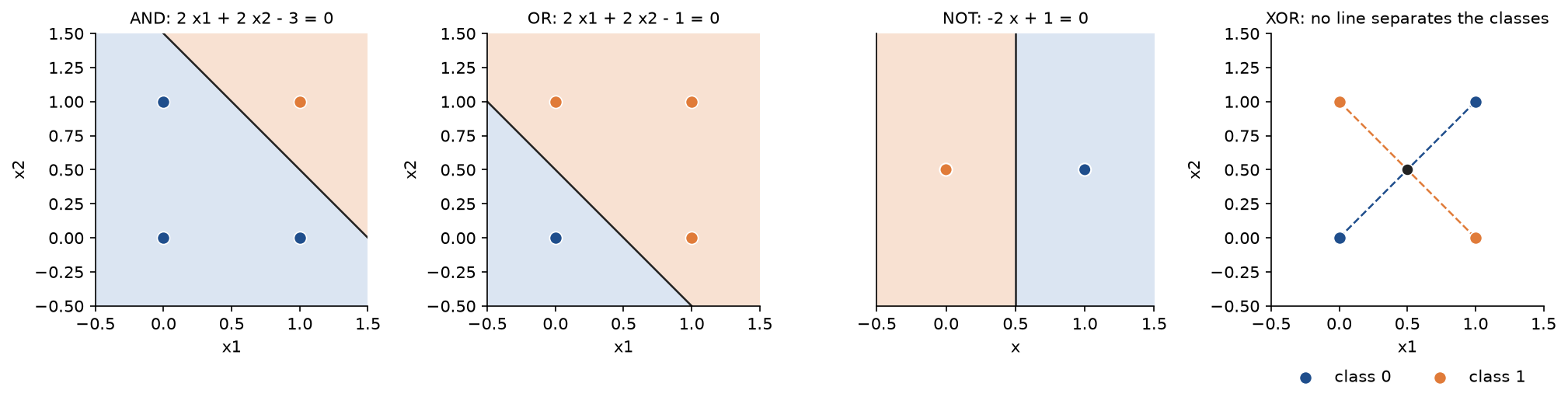
Four panels. AND and OR: the unit square with the region where the gate outputs 1 shaded orange and the rest blue, separated by the gate's line, with the four inputs coloured by their output. NOT: the input axis split at 0.5. XOR: the four inputs with the two diagonals, one joining the blue class-0 points and one joining the orange class-1 points, crossing at the centre

Every input lies at least one unit of net input away from its gate's line, so nothing hangs on the convention at z = 0. The XOR panel shows the crossing diagonals that make a single line impossible; a linear program in examples/logic_gates.py confirms that AND, OR and NAND are separable and XOR is not.

Learning a perceptron by hand¶

Six points, three per class, are visited in this order every epoch:

Example 1: x = (2, 2), class 1, t = +1.
Example 2: x = (-1, 1), class 0, t = -1.
Example 3: x = (4, 3), class 1, t = +1.
Example 4: x = (1, 0), class 0, t = -1.
Example 5: x = (-1, 2), class 1, t = +1.
Example 6: x = (2, -1), class 0, t = -1.

Start from w = (0, 0) and b = 0 with η = 1. Each visit computes z = w x + b with the current weights and checks t z ≤ 0; on a mistake it adds t x to w and t to b. The visits of the first two epochs are:

Epoch 1, example 1: z = 0, so t z = 0, a mistake. Now w = (2, 2), b = 1.
Epoch 1, example 2: z = 1, t z = -1, a mistake. Now w = (3, 1), b = 0.
Epoch 1, example 3: z = 15, t z = 15, correct.
Epoch 1, example 4: z = 3, t z = -3, a mistake. Now w = (2, 1), b = -1.
Epoch 1, example 5: z = -1, t z = -1, a mistake. Now w = (1, 3), b = 0.
Epoch 1, example 6: z = -1, t z = 1, correct.
Epoch 2, example 1: z = 8, correct.
Epoch 2, example 2: z = 2, t z = -2, a mistake. Now w = (2, 2), b = -1.
Epoch 2, example 3: z = 13, correct.
Epoch 2, example 4: z = 1, t z = -1, a mistake. Now w = (1, 2), b = -2.
Epoch 2, example 5: z = 1, t z = 1, correct.
Epoch 2, example 6: z = -2, t z = 2, correct.

In epoch 3 the net inputs are 4, -1, 8, -1, 1 and -2, every t z is positive, and the rule stops after 6 updates, with 4, 2 and 0 mistakes in the three epochs. A few visits in detail. The first example meets the zero weights, so z = 0 and it counts as a mistake. Example 2 then has z = 2 × (-1) + 2 × 1 + 1 = 1 although its class is 0, so w = (2, 2) - (-1, 1) = (3, 1) and b = 1 - 1 = 0. Example 5 is a class-1 point on the wrong side, z = 2 × (-1) + 1 × 2 - 1 = -1, and is added: w = (2, 1) + (-1, 2) = (1, 3). Example 4 needs two corrections: the first moves its t z from -3 to -3 + 2 = -1, since the squared length of (1, 0, 1) is 2, as the update identity predicts, and only the second, in epoch 2, puts it on the correct side. The final separator is the line x1 + 2 x2 - 2 = 0, that is x2 = -x1 / 2 + 1. The y - ŷ rule makes the same six updates here, because no class-0 example ever lands exactly on the boundary.

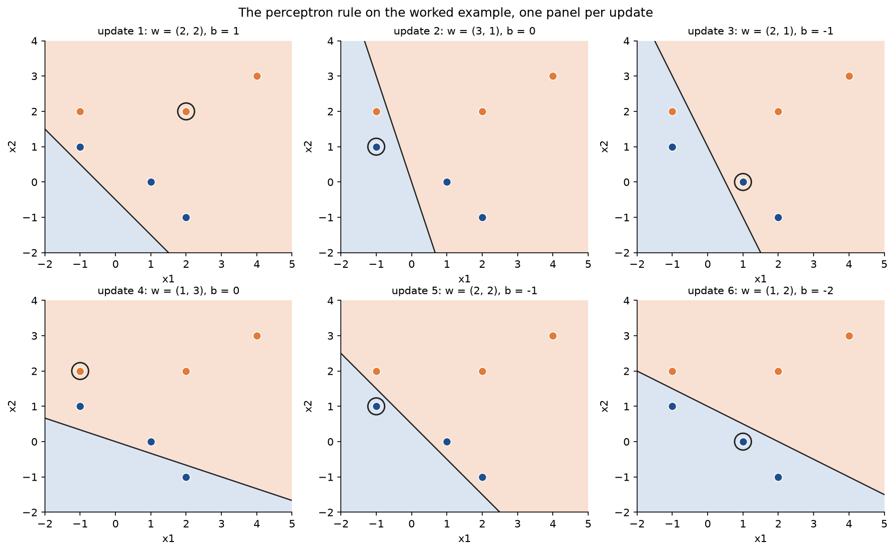
Six panels, one per update, each showing the six points, the line after the update with the side it calls class 1 shaded orange, and a ring around the example that caused the update; the line swings from steep to shallow and ends as x2 = -x1 / 2 + 1 with all points on their correct sides

The rings show which example pulled the line each time; examples 2 and 4, both of class 0, cause two updates each.

The convergence bound for this data¶

The augmented inputs (x, 1) have squared lengths 9, 3, 26, 2, 6 and 6, so R² = 26 and R = 5.0990. Take u to be the separator just found, scaled to unit length: the length of (1, 2, -2) is 3, so u = (1, 2, -2) / 3. The values of t u x̃ for the six examples are 4/3, 1/3, 8/3, 1/3, 1/3 and 2/3, so γ = 1/3 = 0.3333 and the theorem promises at most (R / γ)² = 26 × 9 = 234 updates. The rule made 6. Along the way the two quantities of the proof stay within their bounds, k γ below the projection and k R² above the squared length:

Update 1: weights (2, 2, 1), projection 1.3333 against k γ = 0.3333, squared length 9 against k R² = 26.
Update 2: weights (3, 1, 0), projection 1.6667 against 0.6667, squared length 10 against 52.
Update 3: weights (2, 1, -1), projection 2.0000 against 1.0000, squared length 6 against 78.
Update 4: weights (1, 3, 0), projection 2.3333 against 1.3333, squared length 10 against 104.
Update 5: weights (2, 2, -1), projection 2.6667 against 1.6667, squared length 9 against 130.
Update 6: weights (1, 2, -2), projection 3.0000 against 2.0000, squared length 9 against 156.

Each update raises the projection by exactly t u x̃ of the corrected example, 4/3 for the first and 1/3 for each later one. The squared length stays far below k R² and even drops at update 3, from 10 to 10 + 2 × (-3) + 2 = 6: the proof bounds its growth, not its monotonicity.

For this data the separator the perceptron found happens to be the one with the largest augmented margin. Examples 2, 4 and 5 lie at the margin, and (1, 2, -2) = 5 × (-1) x̃2 + 0.5 × (-1) x̃4 + 3.5 × (+1) x̃5 with positive coefficients, which is the optimality condition of the maximum-margin problem. So 234 is the best bound the theorem gives for these six points, and it is 39 times the true count.

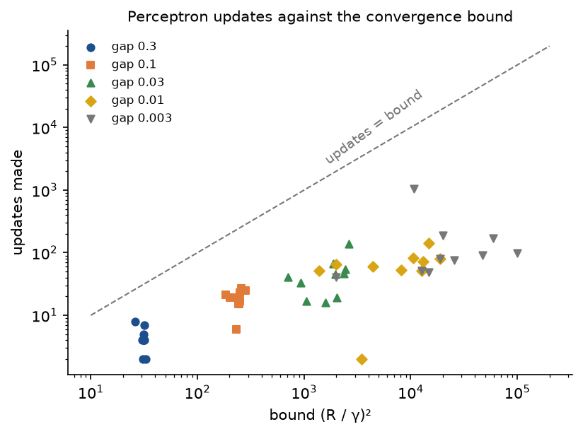
Updates made against the bound for 50 random separable sets of 200 points on logarithmic axes, coloured and shaped by the empty gap around the true line from 0.3 to 0.003; every point lies well below the dashed diagonal where the two would be equal

The gap is typical. On 50 random separable sets of 200 points, visited in a fresh random order every epoch, the updates never exceed 0.305 times the bound, and the gap widens as the margin shrinks: with an empty gap of 0.003 around the true line the median bound is 19,420 updates and the median count 86.

XOR in matrix form¶

The four inputs form a batch X with the rows (0, 0), (0, 1), (1, 0) and (1, 1), one example per row. Through the step network of the section on XOR:

The hidden net inputs Z1 = X W1ᵀ + b1 have the rows (-1, 3), (1, 1), (1, 1) and (3, -1). For the second row, hidden unit 1 computes 2 × 0 + 2 × 1 - 1 = 1 and hidden unit 2 computes -2 × 0 - 2 × 1 + 3 = 1.
The hidden activations A1 = H(Z1) have the rows (0, 1), (1, 1), (1, 1) and (1, 0), the hidden-space points of the figure above.
The output net inputs are -1, 1, 1 and -1, and the outputs 0, 1, 1 and 0, which is XOR.

Now the smooth version: every step replaced by a sigmoid and every weight and bias multiplied by c = 3, so W1 has the rows (6, 6) and (-6, -6), b1 = (-3, 9), W2 = (6, 6) and b2 = -9. The net inputs are three times those above:

The hidden activations are σ(-3) = 0.0474 and σ(9) = 0.9999 for (0, 0), σ(3) = 0.9526 twice for each of (0, 1) and (1, 0), and 0.9999 and 0.0474 for (1, 1).
For the first row the output net input is 6 × (0.0474 + 0.9999) - 9 = -2.7162. For the second it is 6 × (0.9526 + 0.9526) - 9, which is 2.4312 from the rounded terms and 2.4309 at full precision.
The output net inputs are -2.7162, 2.4309, 2.4309 and -2.7162, and the outputs 0.0620, 0.9192, 0.9192 and 0.0620.

The smooth network is right with some confidence to spare. With c = 1 its outputs are 0.3642 and 0.4811, both below one half, so it gets the two class-1 inputs wrong; with c = 10 they agree with XOR to four decimals.

The code¶

The package perceptron_and_mlp is plain NumPy, split into one module per idea. SciPy, scikit-learn and PyTorch are imported only inside the functions that need them.

arrays.py holds the Array type and as_matrix, which insists on one example per row.
activations.py holds the step, sigmoid, tanh, ReLU and identity with their derivatives in ACTIVATIONS, and softmax for output layers.
perceptron.py holds the frozen Perceptron with net_input, predict and augmented_weights, and the helpers signed_labels, augment and decision_line.
gates.py holds LOGIC_GATES with the hand-chosen weights, the reference truth tables GATE_TRUTH, truth_table, and the four binary inputs with the XOR labels.
learning_rule.py holds train_perceptron, with a fixed or seeded random order, either convention at z = 0 and optional recording of every step, and format_perceptron_trace, which prints a run as above.
convergence.py holds data_radius, margin, mistake_bound, proof_quantities and margin_support, the SciPy checks is_linearly_separable (a linear program) and max_margin_separator (quadratic programming), and bound_experiment for random data.
datasets.py generates the worked points, random separable sets and the two spirals from a seed.
propagation.py holds the batch forward pass, the matched costs and the backward pass as plain functions of the parameters.
network.py holds the frozen MLP class with forward, forward_one for a single column vector, cost, gradients, step, classify and parameter_count, and initialize_mlp.
training.py runs mini-batch gradient descent with a reproducible batch order and measures accuracy; gradient_check.py compares the gradients with central differences.
xor.py builds the hand-made XOR network in its step and sigmoid versions, fits XOR with an affine map, and trains small networks on XOR from random starts.
approximation.py holds the ReLU interpolant, the sigmoid staircase, their error bounds and sup_error; depth.py holds the linear collapse, the sawtooth networks, count_linear_pieces and the widths that fit a parameter budget.
comparisons.py holds the copies to and from scikit-learn's Perceptron and MLPClassifier and PyTorch's nn.Sequential.
plotting.py, perceptron_plots.py and network_plots.py draw every figure in the handbook's four colours.

Python counts from zero, so weights[0] is W1, and activations[l] of a forward pass is the activation of layer l, starting with the inputs. The heart of the learning rule is

z = float(x @ weights + bias)
if boundary_is_mistake:
    mistake = t * z <= 0.0
else:
    mistake = (t > 0.0 and z <= 0.0) or (t < 0.0 and z > 0.0)
if mistake:
    weights = weights + learning_rate * t * x
    bias = bias + learning_rate * t

and the forward pass is the matrix form above, one line per equation:

for w, b, name in zip(weights, biases, activations):
    z = a @ w.T + b
    a = activation_function(name)(z)

The examples and the project import the package, so install the repository first as described in the main README. Each example demonstrates one idea; three run in a few seconds, and the three that train many networks take ten to fifteen seconds:

examples/logic_gates.py prints the truth tables and lines of the gates, shows that NOT needs a bias, checks separability with a linear program and watches the rule cycle on XOR.
examples/perceptron_rule.py prints the worked trace, the bound and the quantities of the proof, the largest-margin separator, the bound against the true count on random data, the rescaling by the learning rate and the effect of the convention at z = 0.
examples/xor_hidden_layer.py runs the XOR networks in matrix form, shows the zero gradients of step units, the collapse of linear layers, the network learned by gradient descent and the success rate of random starts.
examples/universal_approximation.py builds both constructions for growing widths, compares their errors with the bounds and with trained networks, and measures the error outside the interval.
examples/depth_versus_width.py counts the pieces of shallow and deep ReLU networks and prints the sizes each needs for the same sawtooth.
examples/compare_with_libraries.py checks the rule against scikit-learn's Perceptron, the forward pass and SGD steps against MLPClassifier, and the forward pass and gradients of a trained network against PyTorch.

python neural-networks/perceptron-and-mlp/examples/logic_gates.py
python neural-networks/perceptron-and-mlp/examples/perceptron_rule.py
python neural-networks/perceptron-and-mlp/examples/xor_hidden_layer.py
python neural-networks/perceptron-and-mlp/examples/universal_approximation.py
python neural-networks/perceptron-and-mlp/examples/depth_versus_width.py
python neural-networks/perceptron-and-mlp/examples/compare_with_libraries.py

The sample project, project/spiral_classifier.py, applies everything to a problem no line can solve. It generates two interleaved spirals of 250 points each with two and a quarter turns and noise of standard deviation 0.04, and a second draw with the next seed as the test set. The two arms are images of each other under a half turn about the origin, so any line through the origin classifies about half the points correctly. It trains a perceptron as the baseline, then for every depth in --depths a network whose hidden layers share one width chosen so that the parameter count comes closest to --budget, from --restarts random starts each. By default these are a wide network of one hidden layer with 84 tanh units and a deep network of two hidden layers with 16, both with exactly 337 parameters, a sigmoid output and the cross-entropy cost, trained by mini-batch gradient descent with batches of 16, learning rate 0.1 and 2,000 epochs. Before the first start of each network it checks the gradients on eight examples. Options such as --depths, --budget, --activation, --epochs and --restarts change the setup, and --figures sends the three PNGs to another folder so a custom run does not overwrite the ones shown here; the default run takes about 20 seconds.

python neural-networks/perceptron-and-mlp/project/spiral_classifier.py
python neural-networks/perceptron-and-mlp/project/spiral_classifier.py --depths 1 2 3 4

With the defaults the results are:

The perceptron never converges. After 100 epochs it still makes 232, 240 and 238 mistakes per epoch, and its last weights classify 59.0 % of the training points and 54.8 % of the test points correctly.
The wide 2-84-1 network ends at training costs 0.1464, 0.1655 and 0.2498 from its three starts, with training accuracies 0.9620, 0.9600 and 0.8700 and test accuracies 0.9160, 0.8840 and 0.8340, a mean of 0.8780.
The deep 2-16-16-1 network ends at training costs 0.0047, 0.0097 and 0.0057, with training accuracies 1.0000, 0.9980 and 1.0000 and test accuracies 0.9940, 0.9860 and 0.9800, a mean of 0.9867.

With this budget the deeper network wins from every start. That is one problem and one training budget, not a law, but it matches the counting argument: following a spiral needs many folds, and composing layers produces folds far more cheaply than adding units side by side. The second command extends the comparison: three hidden layers of 12 units (361 parameters) fit the training set from two of three starts but reach a mean test accuracy of 0.9713, and four hidden layers of 9 units (307 parameters) stall at training costs around 0.2 with a mean test accuracy of 0.8553. Layers that narrow and that many tanh layers deep are hard for plain gradient descent to train, so depth pays only up to a point.

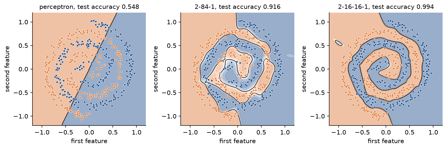
Decision regions on the test points for the perceptron, the 2-84-1 network and the 2-16-16-1 network, each from its first start: the perceptron splits the plane with one straight line at test accuracy 0.548, the wide network follows the arms roughly with gaps and stray islands at 0.916, and the deep network traces both spiral arms cleanly at 0.994, apart from one small island outside the data

The shading is the predicted probability of class 1 and the black curve its 0.5 contour. The wide network gets the outer turns right but blurs the centre, where the arms are close together and change direction fastest. Both networks also draw small islands far from any training point, where nothing constrains them.

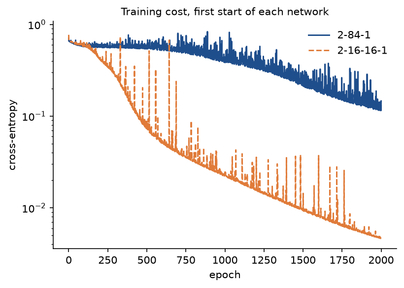
Training cross-entropy over 2,000 epochs on a logarithmic axis for the first start of the two networks: the wide network creeps down to about 0.15 with heavy noise, the deep network drops below 0.01, with occasional short spikes

The deep network's cost ends about thirty times lower. The spikes are mini-batch steps that briefly overshoot; plain gradient descent with a constant learning rate recovers from each of them.

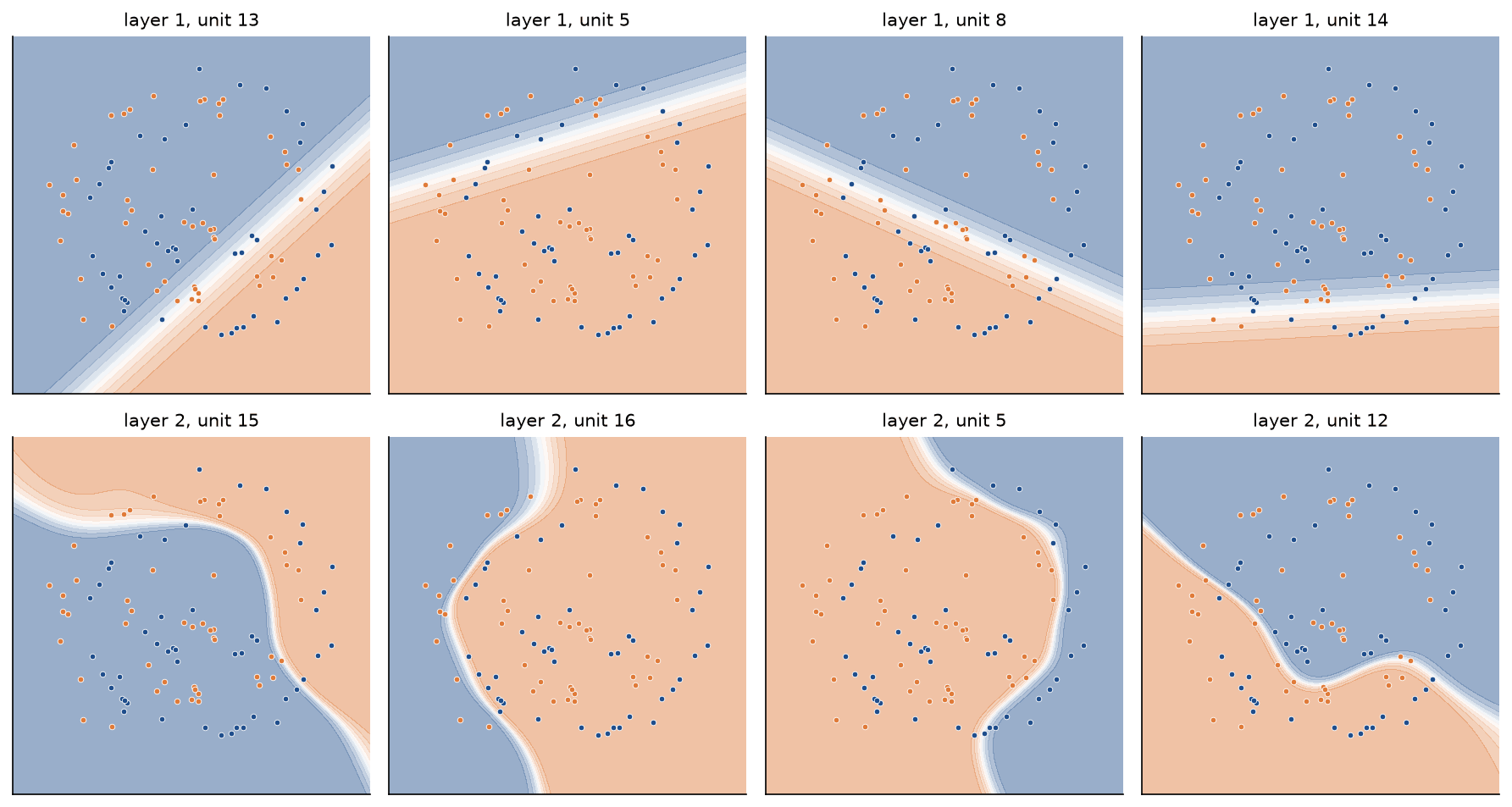
Activations of the four hidden units with the largest outgoing weights in each layer of the trained 2-16-16-1 network, over the input plane: first-layer units are soft half-planes with straight edges, second-layer units are regions with curved edges

The hidden units show what each layer computes. Every first-layer unit is tanh of an affine function of the input, a soft half-plane that changes only across one direction. Every second-layer unit combines sixteen of them into a region with a curved edge, and the output unit combines those into the spiral.

The notebook perceptron_and_mlp.ipynb is a guided tour in the order of this page: the logic gates, the learning rule and its bound, XOR and its two-layer network, sigmoid neurons, the forward pass in matrix form, XOR learned by gradient descent, the universal approximation constructions, depth against width, the pitfalls below, the spirals and the library comparison. The tests in tests check the worked example value by value, the mathematical properties above and the agreement with scikit-learn and PyTorch, and run in a few seconds:

python -m pytest neural-networks/perceptron-and-mlp

Every dataset on this page is synthetic, generated from a seed by worked_points, separable_data and two_spirals, so nothing is downloaded and no licence is involved.

In practice¶

Nobody trains a single perceptron in production, and multilayer networks are written in a deep learning framework. The from-scratch code agrees with the libraries exactly where it should, as examples/compare_with_libraries.py shows:

from perceptron_and_mlp import sklearn_perceptron, train_perceptron, worked_points

inputs, labels = worked_points()
model = sklearn_perceptron(inputs, labels, epochs=5)
print(model.coef_, model.intercept_)
print(train_perceptron(inputs, labels).perceptron.augmented_weights)

sklearn.linear_model.Perceptron implements the rule with the update at z = 0 included: it is stochastic gradient descent on the perceptron criterion with learning rate eta0. With penalty=None, eta0=1, shuffle=False and tol=None it ends with exactly our weights (1, 2) and bias -2 on the worked example, and with weights identical to the last bit after 20 epochs on the spirals, where neither converges. Its defaults shuffle the data every epoch and stop when the training loss stops improving by tol, which is not the same as reaching zero mistakes.
sklearn.neural_network.MLPClassifier stores the weights of layer l in coefs_[l - 1] with shape (inputs, outputs), the transpose of our W. After copying our initial 2-16-16-1 network into it, its predicted probabilities agree with ours to 1.1 × 10⁻¹⁶, and with plain SGD (momentum=0, alpha=0, shuffle=False) five epochs of partial_fit reproduce five epochs of train_mlp to 2.2 × 10⁻¹⁶ in every weight. Trained from its own start with the project's settings, it reaches 0.9980 on the training set and 0.9760 on the test set, against 1.0000 and 0.9940 for our first start. Its loss_curve_ averages the batch losses seen during each epoch, so it differs from the end-of-epoch cost that train_mlp records.
A PyTorch nn.Sequential of nn.Linear layers uses our (outputs, inputs) layout. to_torch copies a network into it; on the trained deep network the outputs agree with ours to 2.0 × 10⁻¹⁵ over the test set and autograd's gradients to 1.5 × 10⁻¹⁶ on a batch of 32.

When to use which:

Use the from-scratch code to see each idea work: the rule and its bound, the hidden-space construction, the approximation and depth arguments. Every function is small enough to read.
Use sklearn.linear_model.Perceptron only as a baseline; for a linear classifier in earnest prefer logistic regression or a linear support vector machine, which also behave sensibly on data that no line separates.
Use MLPClassifier for small tabular problems where a few lines of code matter more than control; it trains with SGD, Adam or L-BFGS but exposes no gradients or custom layers.
Use PyTorch for anything larger or anything non-standard. MNIST from scratch builds a complete classifier both ways.

Pitfalls¶

Expecting a perceptron to learn XOR. On data that no hyperplane separates, the rule never stops and the last weights can be poor. On XOR in the order (0, 0), (0, 1), (1, 0), (1, 1) the four updates of every epoch cancel exactly, so the weights return to zero after each epoch forever, as examples/logic_gates.py prints. Check separability first, with a linear program as is_linearly_separable does, or use a method designed for overlapping classes.
Tuning the learning rate of a perceptron started at zero. It only rescales the weights: the mistakes and predictions are identical for every η > 0, and examples/perceptron_rule.py prints the same three epochs for η = 0.01, 1 and 100. It does matter for a nonzero start and for every gradient-based method.
Ignoring the convention at z = 0. Whether a point exactly on the boundary counts as a mistake changes the run. On the five points (3, 3) and (2, 2) of class 1 and (-1, 1), (2, 0) and (1, -1) of class 0, the rule used here stops at w = (1, 1), b = -3 after 5 updates and the y - ŷ rule at w = (0, 2), b = -2 after 4, with the class-0 point (-1, 1) left exactly on its line (examples/perceptron_rule.py). Hand calculations often hit z = 0 at the very first step from zero weights without saying which convention they use.
Leaving out the bias. Without it every boundary passes through the origin, and NOT becomes impossible: the input 0 has net input 0 whatever the weight, so the unit outputs 0 for it (examples/logic_gates.py).
Believing that small weight changes give small output changes in a perceptron. That is the property of the sigmoid neuron. A threshold unit's output is piecewise constant in the weights, so its gradient is zero: the backward pass through the step-activation XOR network returns all-zero gradients even when every target is flipped (examples/xor_hidden_layer.py).
Stacking layers without nonlinear activations. Any number of linear layers is one affine map, and the best affine fit to XOR outputs 0.5 for every input (examples/xor_hidden_layer.py, notebook section "The forward pass in matrix form").
Too few hidden units, or one unlucky start. The cost of a network is not convex. A 2-2-1 sigmoid network solves XOR from 39 of 50 random starts, a 2-3-1 network from 48 and a 2-4-1 network from all 50; the failed runs end on a plateau with cost about 0.3484 (examples/xor_hidden_layer.py). Use a few more hidden units than a hand construction needs, or several restarts.
Reading the universal approximation theorem as a promise about learning. It guarantees that good weights exist on a bounded region. The width-64 ReLU interpolant is within 0.0047 of the target on [-2, 2] and 1.7750 off on [2, 3], and tanh networks trained by gradient descent stall near an error of 0.15 from 16 units on, while the construction with 128 units reaches 0.0012 (examples/universal_approximation.py).
Making a deep network too narrow. Depth multiplies the pieces a network can form, but four tanh layers of 9 units train far worse on the spirals than two layers of 16 with about the same budget (project/spiral_classifier.py --depths 1 2 3 4).
Copying weights between libraries without transposing. scikit-learn's coefs_ are (inputs, outputs); our W and torch.nn.Linear.weight are (outputs, inputs). For square layers the wrong orientation raises no error and silently computes a different network; to_sklearn_mlp and from_sklearn_mlp transpose explicitly, and examples/compare_with_libraries.py prints both sets of shapes.