Object detection

A classifier says what is in an image; a detector says what is where. Its output is a set of boxes, each with a class and a score, and the number of objects is not known in advance. That one change brings a family of problems with it: describing a box, deciding when two boxes describe the same object, removing the duplicate boxes a dense predictor produces, turning a grid of network outputs into boxes and back, and scoring one set of boxes against another. This page derives the overlap measures IoU, GIoU and DIoU, greedy and soft non-maximum suppression, anchor matching, the YOLO-style grid encoding with sigmoid offsets and exponential sizes, the box-regression parameterization of the R-CNN family and the common definitions of average precision. Every step is worked through with small numbers, implemented in NumPy and tested, and a small grid detector is then trained on synthetic coloured shapes and scored with the same code. Afterwards you will be able to compute any of these quantities on paper, read the post-processing and evaluation code of a real detector, and notice when a reported mAP is not the number it claims to be. It builds on Convolutional networks, which supply the feature maps every modern detector starts from.

To run the code in this topic, install the base group, the deep group for the shape detector and the autograd comparison, and the ml group for the comparison with scikit-learn.

Intuition

A box is four numbers, and there are several ways to choose them: two corners, or a centre with a width and a height, in pixels or as fractions of the image. Mixing two conventions produces boxes that look valid and are wrong, so every function on this page states which form it takes.

Two boxes describe the same object when they overlap enough. The standard measure is intersection over union, IoU: the area they share divided by the area they cover together. It is 1 for identical boxes and 0 for disjoint ones, and it does not care about the size of the boxes, so a 5-pixel error on a small object counts for more than on a large one. A detection is usually called correct when its IoU with a ground-truth box is at least 0.5.

A detector does not look for objects one at a time. It scores thousands of candidate boxes at once, at every position of a grid and for several reference shapes per position, so one object lights up many neighbouring candidates. Non-maximum suppression, NMS, cleans this up greedily: keep the best-scoring box, delete every box that overlaps it too much, repeat.

The reference shapes are anchors. Instead of predicting a box from nothing, the network predicts a small correction to an anchor: a shift of its centre and a rescaling of its width and height. During training each ground-truth box is handed to the anchors that resemble it, measured again by IoU, and those anchors learn to reproduce it. Two-stage detectors of the R-CNN family use the same idea twice: a first stage proposes regions, a second stage classifies each region and corrects its box.

Finally, a detector is scored by sorting all its detections by confidence and walking down the list. Each detection either finds a new object, a true positive, or not, a false positive. That traces a precision-recall curve, and average precision, AP, summarizes the curve in one number per class. The mean over classes is mAP. The details of the summary differ between benchmarks, and the differences are larger than many of the improvements reported with them.

The diagram shows where each piece sits. Solid arrows run at inference time and dashed orange arrows only during training. A one-stage detector takes the upper path, a two-stage detector the lower one, and both end in the same decoding and suppression.

Evaluation runs offline and needs ground truth. Note the second arrow from the ground truth: recall divides by every object of the class, including those that no detection ever finds.

How it works

Notation and box formats

Image coordinates have x to the right and y downwards, with the origin at the top-left corner of the image. Coordinates are continuous: a pixel covers a unit square, so a box from x1 = 2 to x2 = 5 is 3 wide. The quantities used below are:

• Corner form (x1, y1, x2, y2): the top-left and bottom-right corners, with x2 at least x1 and y2 at least y1.
• Centre form (bx, by, bw, bh): the centre, the width and the height.
• |B| for the area of a box B, A ∩ B and A ∪ B for the region two boxes share and the region they cover, and C for the smallest axis-aligned box enclosing both.
• ρ for the distance between the centres of A and B, and d for the length of the diagonal of C.
• τ for an IoU threshold.
• S for the grid size in cells per side, s for the stride in pixels (the image size divided by S), and (cx, cy) for the column and row of a cell.
• (pw, ph) for the width and height of an anchor or proposal, and tx, ty, tw, th for the raw network outputs of one box.
• σ for the logistic sigmoid.
• Pk and Rk for precision and recall after the k highest-scoring detections, and N for the number of ground-truth boxes of a class.

The two main forms convert into each other by halving the size on either side of the centre:

A third form is common in annotation files: COCO stores (x1, y1, bw, bh), the top-left corner with the size. YOLO label files store the centre form divided by the image width and height, so every number lies between 0 and 1. Areas and intersections are simplest in corner form, the encodings below are simplest in centre form.

Intersection over union and its extensions

The intersection of two axis-aligned boxes is itself a box, or empty. Its width is the overlap of the two intervals on the x axis, from the larger left edge to the smaller right edge, clipped at zero, and its height likewise. The union follows by inclusion and exclusion:

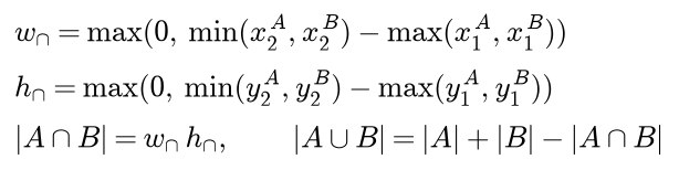
IoU is their ratio:

IoU lies between 0 and 1, is symmetric, and does not change when both boxes are shifted or scaled by the same factor. One minus IoU is the Jaccard distance, a true metric. Its weakness is that it is exactly zero for every pair of disjoint boxes, however far apart, so as a training loss 1 - IoU gives no gradient until the predicted box already touches its target.

Generalized IoU subtracts the share of the enclosing box C that neither box covers:

When one box contains the other, C is the union and GIoU equals IoU. As two boxes move apart the empty share approaches 1, so GIoU lies between -1 and 1 and keeps decreasing with distance after IoU has stopped at zero. It can be negative even for overlapping boxes, when they cover an L-shaped region whose enclosing box is mostly empty.

Distance IoU subtracts the squared distance between the centres, divided by the squared diagonal of C so that the penalty does not depend on scale:

The penalty pulls centres together directly, which in its authors' experiments makes training converge faster than with GIoU, whose penalty can also be reduced by first growing the predicted box. Complete IoU, CIoU, adds a third term for the mismatch of aspect ratios. Each measure gives a box loss of the form one minus the measure.

Non-maximum suppression

Greedy NMS with threshold τ keeps the highest-scoring remaining box, removes every remaining box whose IoU with it is greater than τ, and repeats until no boxes remain.

The removed boxes are those that overlap the kept box by more than the threshold. Boxes that overlap it little are left alone, because they may be other objects. Whether a box with IoU exactly τ is removed is a convention that matters only for exact ties; the package and torchvision.ops.nms keep it.

Two boxes of different classes are not duplicates of each other: a person standing in front of a car may overlap the car's box heavily. Detectors therefore run NMS separately for each class, called per-class or batched NMS. Pooling all classes together is called class-agnostic NMS and suits classes that cannot overlap in space. Greedy NMS compares every kept box with every remaining box, so it costs a number of IoU evaluations that grows with the square of the number of candidates, which is why a score threshold is applied first.

The hard cut has a cost in crowded scenes: two real objects whose boxes overlap by more than τ cannot both survive. Soft-NMS replaces the deletion by a decay of the score. With M the box just kept and Bi every remaining box with score si:

The next box kept is the one with the highest decayed score. A heavily overlapping box ends up with a low score rather than none, and the score threshold applied afterwards, or the evaluation itself, decides what that means. Greedy NMS is the special case whose decay factor is 0 above τ and 1 below it.

Anchors and matching

An anchor is a fixed reference box. A detector places k anchors of chosen widths and heights at the centre of every cell of a feature map, which gives S times S times k anchors per feature map, and predicts for each one a class score and a correction of the box. Training needs a rule that says which anchors should predict which ground-truth box. The rule of Faster R-CNN's region proposal network, SSD and RetinaNet compares every anchor with every ground-truth box by IoU and uses two thresholds, a lower one and an upper one:

• An anchor whose best IoU reaches the upper threshold is positive and learns that ground-truth box.
• An anchor whose best IoU is below the lower threshold is negative and learns the background class.
• An anchor in between is ignored and contributes nothing to the loss.
• Afterwards every ground-truth box also claims its single best anchor, even below the upper threshold, so that small or oddly shaped objects are not left without one.

RetinaNet uses 0.5 and 0.4, the region proposal network 0.7 and 0.3. Almost all anchors end up negative, which is why one-stage detectors need a remedy for class imbalance. SSD keeps only the hardest negatives, at three negatives per positive. RetinaNet's focal loss down-weights the many easy ones, where pt is the probability the model gives the correct class and γ, typically 2, sets how strongly confident predictions are discounted:

YOLO-style detectors use a simpler rule. The cell that contains the centre of a ground-truth box is responsible for it, and among that cell's anchors the one whose shape fits best predicts it. Shape is compared with both boxes centred on the same point, which turns IoU into a function of the widths and heights alone:

Good anchor shapes can be learned from the data: k-means clustering of the training boxes' widths and heights with the distance one minus shape IoU gives anchors that match the typical objects, the recipe introduced with YOLOv2. Clustering covers k-means itself.

YOLO-style encoding and decoding

For the anchor in cell (cx, cy) with size (pw, ph), the network outputs four box numbers tx, ty, tw, th, an objectness logit to and one logit per class. Decoding turns them into a box in pixels with the sigmoid; encoding will need its inverse, the logit:

The objectness is σ(to), the class probabilities π are a softmax over the class logits ℓ, or one sigmoid per class when a box may carry several labels, and the score of the box for class k is the objectness times the probability of class k:

One image therefore gives an output tensor of shape S by S by k by (5 + K) for K classes.

Each choice has a reason. The sigmoid keeps the offset between 0 and 1, so the predicted centre can never leave its cell; without it, an early, untrained network can place a box anywhere, and training is unstable. The exponential keeps widths and heights positive, and it makes the size error symmetric on a log scale: predicting half the true width costs as much as predicting twice the width.

Encoding inverts decoding. For a ground-truth box in centre form, the responsible cell is the integer part of the centre divided by the stride, and the offset u is what remains. Solving the decoding equation for tx gives σ(tx) = ux, so the target is the logit of the offset, and the size targets are logarithms of ratios:

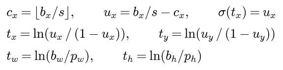
The logit is infinite at u = 0, a centre exactly on a cell boundary, so the package clips u to the range from 10⁻⁶ to 1 - 10⁻⁶ before taking it. Training usually avoids the logit altogether by comparing σ(tx) with ux directly, with a squared error or a binary cross-entropy whose gradient with respect to tx is simply σ(tx) - ux, as in logistic regression. The shape detector at the end of this page does that.

The R-CNN family and box regression

R-CNN (2014) turned a convolutional classifier into a detector in the most direct way. Selective search, a hand-designed grouping of superpixels, proposes about 2000 regions per image; each region is cropped, warped to the fixed input size of an ImageNet-pretrained network and passed through it; a linear SVM per class scores the features; and a regressor per class corrects the box. Every proposal costs a full forward pass, so an image costs about 2000 of them, and the pieces are trained separately.

Fast R-CNN (2015) runs the backbone once per image. Each proposal is projected onto the shared feature map, and RoI pooling max-pools the features under it into a fixed grid, for example 7 by 7, so every region, whatever its size, yields a feature tensor of the same shape. A small network on top has two sibling outputs, a softmax over the K classes plus background and box corrections for every class, trained together with a multi-task loss. Here p is the predicted class distribution, u the true class, the bracket [u ≥ 1] switches the box term off for background regions, the sum runs over the four box targets x, y, w and h, and d* are the regression targets defined below:

The proposals still come from selective search, which now dominates the running time. Faster R-CNN (2015) learns the proposals too. A region proposal network slides a small convolution over the shared feature map and predicts, at every position and for each of 9 anchors (three sizes times three aspect ratios), an objectness score and four box corrections, using the matching rule above with thresholds 0.7 and 0.3. Its proposals are cleaned up by NMS at 0.7, and the best few hundred go to the Fast R-CNN head. Proposals now cost almost nothing, and the whole detector trains end to end. Mask R-CNN later replaced RoI pooling by RoIAlign, which samples the feature map bilinearly instead of rounding coordinates to the grid, and added a mask branch; feature pyramid networks attach the heads to several feature-map resolutions so that small and large objects are each handled at a suitable scale.

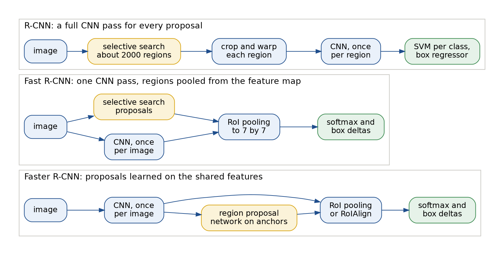
Read from top to bottom, the diagram shows the expensive steps disappearing one at a time: first the per-region CNN pass, then the hand-designed proposals, highlighted in amber.

All three correct a proposal P towards its ground-truth box G with the same parameterization. With (px, py, pw, ph) the centre form of the proposal and (gx, gy, gw, gh) that of the ground truth, the targets are

and a prediction d is decoded with the inverse:

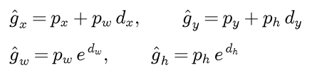
Horizontal quantities are divided by the proposal's width and vertical quantities by its height, never the other way round. That makes the targets invariant to shifting both boxes and to scaling both by the same factor, so a regressor learns one correction for a given relative error whatever the size of the object. The size terms are logarithms for the same reason as the exponential in the YOLO decoding. Implementations often multiply the four targets by fixed weights, (10, 10, 5, 5) in torchvision's Faster R-CNN box head, to bring them to unit scale, and clip dw and dh before the exponential so that an untrained network cannot produce an overflow.

One-stage, two-stage and what came after

A two-stage detector first proposes regions and then classifies and refines each one; a one-stage detector predicts classes and boxes for every anchor of a dense grid in a single pass. YOLO (2016) divided the image into a 7 by 7 grid whose cells regress boxes directly; YOLOv2 added anchors from k-means and the sigmoid offsets above; SSD (2016) placed default boxes on several feature maps of different resolution; RetinaNet (2017) showed that the accuracy gap to two-stage detectors came from the imbalance between a handful of positive and a hundred thousand easy negative anchors, and closed it with the focal loss.

The two designs differ in a few concrete ways:

• Candidates: a two-stage detector such as Faster R-CNN, Mask R-CNN or Cascade R-CNN classifies a few hundred proposals per image, while a one-stage detector such as YOLO, SSD or RetinaNet scores every anchor or grid location, often more than ten thousand.
• Imbalance: in a two-stage detector the proposal stage filters out most of the background and the head trains on sampled mini-batches of regions; a one-stage detector needs hard negative mining or the focal loss.
• Per-region features: two-stage detectors pool them with RoI pooling or RoIAlign, one-stage detectors read the feature map directly.
• Typical strength: two-stage detectors localize more accurately and extend naturally to masks; one-stage detectors are faster and simpler.

Two later departures change the pieces on this page rather than the overall pipeline.

• Anchor-free detectors drop the reference boxes. FCOS predicts, at every feature-map location inside an object, the distances to the four sides of its box plus a centre-ness score; CenterNet predicts a heatmap of object centres and the box size at each peak, and finding local maxima of the heatmap replaces most of NMS. Recent YOLO-style detectors are also anchor-free and choose their positive locations dynamically during training, with label assignment schemes such as SimOTA or task-aligned label assignment that rank locations by a combination of classification score and IoU rather than by a fixed IoU rule.
• DETR treats detection as set prediction. A transformer decoder turns a fixed number of learned object queries, for example 100, into 100 predictions; during training the Hungarian algorithm finds the one-to-one matching between predictions and ground-truth boxes with the lowest total cost, built from the class probability, an L1 distance and the GIoU, and every unmatched prediction is trained to say "no object". Because each object is matched to exactly one prediction, the model learns not to produce duplicates, and neither anchors nor NMS are needed. The price was slow convergence, which Deformable DETR and its successors reduced.

IoU-based measures stay central in both: GIoU appears in DETR's matching cost and loss, and IoU decides what counts as a correct detection in every benchmark.

Precision, recall and average precision

Evaluation compares a set of detections with a set of ground-truth boxes, separately for each class. Sort the detections of the class by decreasing score, over all images together, and visit them in that order. A detection is a true positive if, among the ground-truth boxes of the same class in the same image that are not yet matched, the one with the highest IoU reaches the threshold τ; that ground-truth box is then marked as matched. Otherwise the detection is a false positive. A second detection of an already matched object is therefore a false positive, and so is a correctly placed box with the wrong class.

After the k highest-scoring detections, with TPk of them true positives:

N counts every ground-truth box of the class, including those no detection ever finds, so recall stops below 1 when some objects are missed. Recall never decreases with k. Precision zigzags: it jumps up at every true positive and decays at every false positive. The interpolated precision, or envelope, removes the zigzag by taking the best precision at any recall at least as large, which gives a non-increasing function of the recall level r:

Average precision summarizes the envelope, and benchmarks disagree on how:

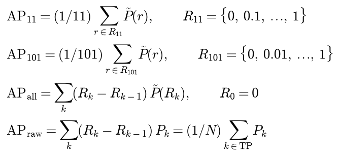
• The 11-point AP was used by PASCAL VOC 2007.
• The all-point AP, the area under the envelope, has been used by PASCAL VOC since 2010.
• The 101-point AP is what COCO computes at each IoU threshold.
• The non-interpolated sum, written AP raw above, is what ranking metrics such as scikit-learn's compute.

In the two sums only the true positives contribute, since recall does not move at a false positive. The mean of AP over the classes that have at least one ground-truth box is mAP. COCO's headline number averages the 101-point mAP over ten IoU thresholds and is reported simply as AP:

COCO also reports AP at single thresholds, AP50 and AP75, and AP for small, medium and large objects, and caps the evaluation at 100 detections per image. The definitions are not ordered: the 11-point value can lie above or below the all-point value depending on where the curve drops, as the worked example and the simulated set below show. Numbers computed with different definitions cannot be compared.

Worked example

Every value is computed in double precision and shown to four decimals; the tests assert each one, and the example scripts print them.

Box formats and overlap

Box A has corners (1, 2, 7, 6) and box B has corners (4, 3, 10, 9). In centre form they are A = (4, 4, 6, 4) and B = (7, 6, 6, 6), in COCO's top-left form (1, 2, 6, 4) and (4, 3, 6, 6), and their areas are 6 × 4 = 24 and 6 × 6 = 36.

• Intersection: x overlaps from max(1, 4) = 4 to min(7, 10) = 7, width 3; y from max(2, 3) = 3 to min(6, 9) = 6, height 3. The intersection is 9.
• Union: 24 + 36 - 9 = 51, so IoU = 9 / 51 = 3 / 17 = 0.1765.
• Enclosing box: from (1, 2) to (10, 9), area 9 × 7 = 63, of which 63 - 51 = 12 is empty. GIoU = 3 / 17 - 12 / 63 = -5 / 357 = -0.0140. The boxes overlap, yet GIoU is negative, because they form an L shape that leaves a fifth of the enclosing box empty.
• Centres (4, 4) and (7, 6): the squared centre distance is 3² + 2² = 13, the squared diagonal of the enclosing box 9² + 7² = 130, and DIoU = 3 / 17 - 13 / 130 = 13 / 170 = 0.0765.

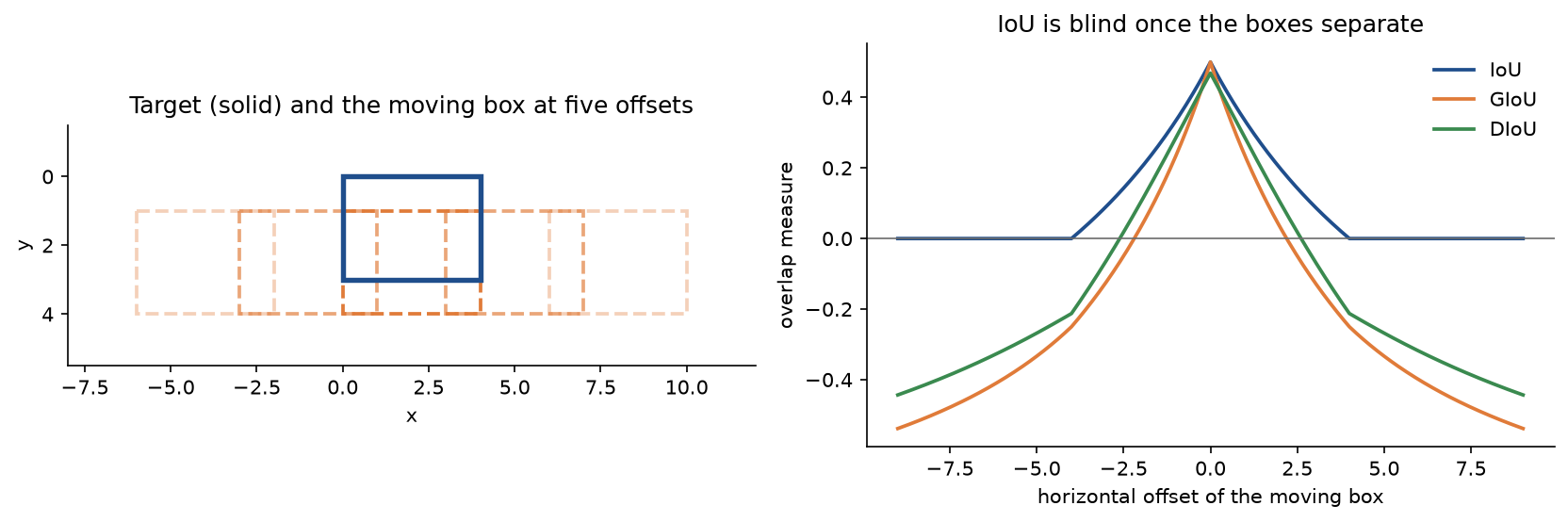
The plot slides a box past a fixed target. Once the boxes separate, IoU cannot tell a near miss from a distant one, while GIoU and DIoU keep falling: at an offset of 6 they are -0.4000 and -0.3190, at 9 they are -0.5385 and -0.4432.

Non-maximum suppression

Six candidate boxes and an NMS threshold of 0.5. A, B and F cover one car, C and E a second car, and D is a person in front of the first car:

• A: corners (24, 28, 72, 74), car, score 0.94.
• B: corners (20, 30, 70, 70), car, score 0.87.
• C: corners (60, 34, 100, 72), car, score 0.76.
• D: corners (30, 26, 64, 76), person, score 0.68.
• E: corners (64, 30, 104, 70), car, score 0.55.
• F: corners (26, 36, 68, 70), car, score 0.41.

Per-class NMS on the cars takes two rounds:

1. Keep A, the highest score. Its IoU with the remaining cars: with B, the intersection is 46 × 40 = 1840 and the union 2208 + 2000 - 1840 = 2368, so 0.7770; with C, 456 / 3272 = 0.1394; with E, 320 / 3488 = 0.0917; with F, which lies entirely inside A, 1428 / 2208 = 0.6467. B and F exceed 0.5 and are removed.
2. Keep C, the better of C and E. IoU(C, E) = 1296 / 1824 = 0.7105, so E is removed.

The result is A and C, one box per car. The person D is handled in its own run and kept, so per-class NMS returns A, C and D. Class-agnostic NMS would remove D, because IoU(A, D) = 1564 / 2344 = 0.6672 is above 0.5.

Gaussian soft-NMS with σ = 0.5 on the cars removes nothing. After A is kept, B's score becomes 0.87 × exp(-0.7770² / 0.5) = 0.2601, C's 0.7310, E's 0.5408 and F's 0.1776. C is kept next and lowers the others again, and so on. The final scores, in the order the boxes are kept, are A 0.9400, C 0.7310, B 0.2534, E 0.1950 and F 0.0625. A score threshold of 0.3 afterwards gives the same two cars as greedy NMS, while a lower one would let the duplicates back in with honest, low scores.

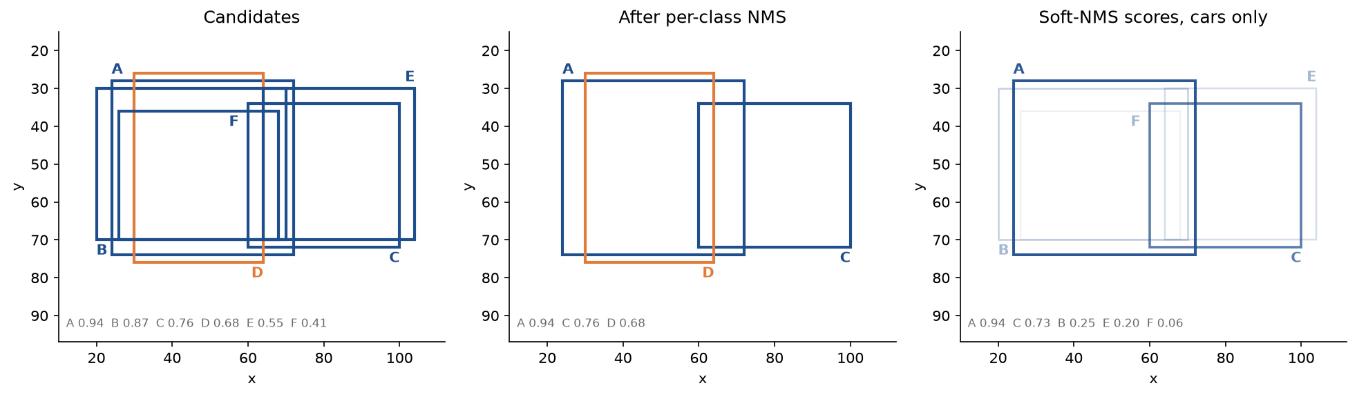
The middle panel is the output of per-class NMS. The right panel shows soft-NMS on the cars: the duplicates survive, but faded to the scores listed along the bottom.

Matching anchors to ground truth

Six anchors and two ground-truth boxes, g1 = (36, 18, 76, 58) and g2 = (60, 62, 84, 94), with the thresholds 0.5 and 0.4:

• a1 = (30, 20, 70, 60): IoU 0.6771 with g1 and 0 with g2, positive for g1 under both rules.
• a2 = (46, 10, 86, 50): IoU 0.4286 with g1, in the ignored band.
• a3 = (50, 30, 90, 70): IoU 0.2945 with g1 and 0.0882 with g2, negative.
• a4 = (10, 50, 50, 90): IoU 0.0363 with g1, negative.
• a5 = (56, 56, 96, 96): IoU 0.0127 with g1 and 0.4800 with g2, ignored under the thresholds alone, positive for g2 with the best-anchor rule.
• a6 = (0, 0, 30, 30): no overlap with either, negative.

For a1, the intersection with g1 is 34 × 38 = 1292 and both boxes have area 1600, so the IoU is 1292 / (3200 - 1292) = 0.6771. The small box g2 lies entirely inside a5, so their IoU is 768 / 1600 = 0.48, in the ignored band. Without the best-anchor rule g2 would have no positive anchor at all, and the detector would never learn it.

Encoding and decoding on a grid

A 128 by 128 image, a 4 by 4 grid with stride 32, three anchors of width and height (20, 36), (48, 28) and (64, 64), and two classes, so the output tensor has shape 4 by 4 by 3 by 7. A ground-truth box of class 1 has centre (75, 50), width 52 and height 30, corners (49, 35, 101, 65). Encoding it:

• Cell: column 75 / 32 rounded down, 2, and row 50 / 32 rounded down, 1; offsets ux = 75 / 32 - 2 = 0.34375 and uy = 50 / 32 - 1 = 0.5625.
• Anchor: the shape IoUs with the three anchors are 600 / 1680 = 0.3571, 1344 / 1560 = 0.8615 and 1560 / 4096 = 0.3809, so anchor 1, the wide one, is responsible.
• Targets: tx = ln(0.34375 / 0.65625) = -0.6466, ty = ln(0.5625 / 0.4375) = 0.2513, tw = ln(52 / 48) = 0.0800 and th = ln(30 / 28) = 0.0690.

The target tensor is zero except at row 1, column 2, anchor 1, which holds (-0.6466, 0.2513, 0.0800, 0.0690, 1, 0, 1): the four box targets, objectness 1 and the one-hot class. Decoding these four numbers gives back (75, 50, 52, 30) exactly.

Now decode a prediction. Suppose the network outputs (tx, ty, tw, th) = (0.2, -0.4, 0.3, -0.1), objectness logit 1.5 and class logits (-0.3, 1.1) at that same cell and anchor. Then σ(0.2) = 0.549834, σ(-0.4) = 0.401312, e to the 0.3 is 1.349859 and e to the -0.1 is 0.904837, shown to six decimals because the stride and the anchor sizes multiply them by up to 48:

• Centre x: 32 × (0.549834 + 2) = 81.5947.
• Centre y: 32 × (0.401312 + 1) = 44.8420.
• Width: 48 × 1.349859 = 64.7932.
• Height: 28 × 0.904837 = 25.3354.

In corner form that is (49.1981, 32.1743, 113.9913, 57.5097). The objectness is σ(1.5) = 0.8176, the class probabilities are (0.1978, 0.8022), and the score for class 1 is 0.8176 × 0.8022, which is 0.6559 from the rounded factors and 0.6558 at full precision. The decoded box overlaps the ground truth with IoU 0.5728: a correct detection at τ = 0.5, not at 0.75.

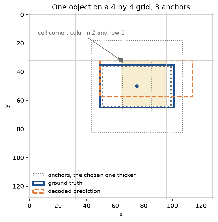
The centre of the ground truth falls in the shaded cell, so only that cell's anchors may predict it. The decoded prediction sits a few pixels off, which is exactly why it passes at IoU 0.5 and fails at 0.75.

R-CNN box regression

A proposal with centre (60, 45), width 40 and height 70, corners (40, 10, 80, 80), and a ground-truth box with centre (66, 40), width 50 and height 56, corners (41, 12, 91, 68). Their IoU is 2184 / 3416 = 0.6393. The regression targets are:

• dx = (66 - 60) / 40 = 0.1500.
• dy = (40 - 45) / 70 = -0.0714.
• dw = ln(50 / 40) = 0.2231.
• dh = ln(56 / 70) = -0.2231.

Decoding them returns the ground-truth box. The two size terms are equal and opposite because 50 / 40 = 1.25 and 56 / 70 = 0.8 = 1 / 1.25. With the weights (10, 10, 5, 5) the targets become (1.5, -0.7143, 1.1157, -1.1157) and decode to the same box.

Average precision on a tiny case

One class, two images and four ground-truth boxes: g1 = (10, 10, 50, 50) and g2 = (60, 20, 90, 70) in image 0, g3 = (20, 30, 60, 60) and g4 = (65, 55, 95, 95) in image 1, so N = 4. Six detections, already sorted by score, matched at τ = 0.5:

1. Score 0.95, image 0, box (11, 11, 51, 50): best IoU 0.9280 with g1, a true positive. Precision 1.0000, recall 0.25, envelope 1.0000.
2. Score 0.83, image 1, box (24, 32, 64, 64): IoU 0.6848 with g3, a true positive. Precision 1.0000, recall 0.50, envelope 1.0000.
3. Score 0.74, image 0, box (16, 4, 52, 46): IoU 0.6483 with g1, but g1 is taken, so a false positive. Precision 0.6667, recall 0.50, envelope 0.6667.
4. Score 0.66, image 1, box (0, 70, 30, 98): no overlap, a false positive. Precision 0.5000, recall 0.50, envelope 0.6667.
5. Score 0.52, image 0, box (60, 34, 92, 80): IoU 0.5708 with g2, a true positive. Precision 0.6000, recall 0.75, envelope 0.6667.
6. Score 0.31, image 1, box (68, 57, 98, 96): IoU 0.7634 with g4, a true positive. Precision 0.6667, recall 1.00, envelope 0.6667.

Detection 3 overlaps g1 well, but g1 already belongs to detection 1, so it is a duplicate and counts against the detector. The four summaries:

• 11-point: the envelope is 1 at the six recall levels 0, 0.1 up to 0.5 and 2/3 at the five levels 0.6 up to 1, so the AP is (6 + 5 × 2/3) / 11 = 28 / 33 = 0.8485.
• All-point: the recall rises by 0.25 at each true positive, where the envelope is 1, 1, 2/3 and 2/3, so the AP is 0.25 × (1 + 1 + 2/3 + 2/3) = 5 / 6 = 0.8333.
• 101-point: the 51 recall levels from 0 to 0.50 see an envelope of 1 and the other 50 see 2/3, so the AP is (51 + 50 × 2/3) / 101 = 0.8350.
• Non-interpolated: (1 + 1 + 0.6 + 0.6667) / 4 = 0.8167, lower than all-point because the precision at rank 5, 0.6, is used as it is instead of being lifted to the 0.6667 that rank 6 reaches.

The 11-point value is the largest here because 6 of its 11 samples fall in the stretch where the envelope is 1. COCO-style AP repeats the matching at stricter thresholds. A detection whose IoU falls below the threshold becomes a false positive, and its object stays unmatched. Writing T for a true and F for a false positive in rank order:

• τ = 0.50 and 0.55: TTFFTT, all-point AP 0.8333, 101-point AP 0.8350.
• τ = 0.60 and 0.65: TTFFFT, all-point 0.6250, 101-point 0.6287.
• τ = 0.70 and 0.75: TFFFFT, all-point 0.3333, 101-point 0.3399.
• τ = 0.80, 0.85 and 0.90: TFFFFF, all-point 0.2500, 101-point 0.2574.
• τ = 0.95: FFFFFF, both 0.

At τ = 0.75, for example, only detections 1 and 6 remain true positives: precision is 1, 0.5, 0.3333, 0.25, 0.2 and 0.3333, recall reaches 0.25 at rank 1 and 0.5 at rank 6, and the all-point AP is 0.25 × 1 + 0.25 × 0.3333 = 0.3333. The mean of the 101-point values over the ten thresholds is the COCO-style AP, (2 × 0.8350 + 2 × 0.6287 + 2 × 0.3399 + 3 × 0.2574 + 0) / 10, which is 0.4379 from the rounded terms and 0.4380 at full precision: about half of the AP at 0.5, because this detector finds its objects but places the boxes loosely.

A larger simulated set

simulate_detector imitates a detector on 300 images with one to four objects of three classes, 769 ground-truth boxes in all. Each object is found with probability 0.85, with a jittered box and a high score; a quarter of the found objects get a second, looser box with a lower score; and about one spurious box per image appears with a low score, 1077 detections in all. At IoU 0.5 the four definitions give a mAP of 0.7785 (11-point), 0.8022 (all-point), 0.7997 (101-point) and 0.8009 (non-interpolated), and the COCO-style AP is 0.3862. The all-point APs of the three classes are 0.8145, 0.7755 and 0.8164.

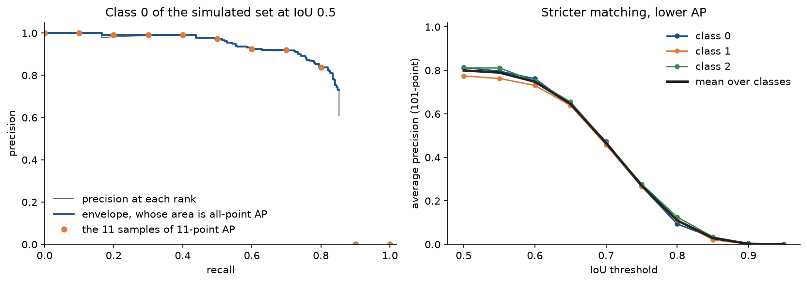
The left panel shows why the 11-point AP is lower here than the all-point AP: the curve ends at recall 0.85, so two of the eleven samples are zero. The right panel shows how strongly the number depends on the matching threshold.

The code

The package object_detection is NumPy throughout, split into one module per idea. PyTorch is imported only inside the functions of detector.py, training.py and comparisons.py, and scikit-learn only inside comparisons.py, so everything else works without them.

• arrays.py holds the array types and the checks for boxes and scores; a box whose corners are reversed raises ValueError.
• boxes.py converts between corner, centre and top-left forms and computes areas, on arrays of shape (..., 4).
• overlap.py holds overlap, which returns every intermediate quantity of the worked example, and box_iou, generalized_iou and distance_iou, pairwise by default and box by box with aligned=True.
• suppression.py holds nms_rounds, which records each round of greedy NMS, non_maximum_suppression, batched_nms for per-class NMS and soft_nms with Gaussian, linear and hard decay.
• anchors.py holds shape_iou, kmeans_anchors, grid_anchors and match_anchors with the NEGATIVE and IGNORED labels.
• yolo_grid.py holds YoloGrid, the sigmoid and logit, encode_offsets and decode_offsets, assign_to_grid and encode_targets, which builds the target tensor of one image.
• decoding.py holds decode_output and postprocess, which turn a raw output tensor into scored, suppressed boxes.
• box_regression.py holds encode_deltas and decode_deltas, with optional weights.
• detections.py holds the GroundTruth and Detections containers, one row per box with its image id.
• matching.py, average_precision.py and evaluation.py hold the three steps of evaluation: match_detections; precision_recall, precision_envelope and average_precision with the methods in AP_METHODS; and evaluate for per-class AP and mAP and coco_average_precision.
• simulation.py generates random boxes and the simulated detector, and shapes.py renders the synthetic shape images with their tight boxes.
• detector.py and training.py build, train and run the small grid detector in PyTorch.
• worked_examples.py builds every example above, so the tests, scripts and notebook share the same numbers.
• pitfalls.py holds deliberately wrong versions of the methods for the Pitfalls section.
• comparisons.py checks the overlap losses against PyTorch's autograd and AP against scikit-learn.
• plotting.py and scenes.py draw every figure in the handbook's four colours and save it reproducibly.

The output tensor of a grid detector is indexed [row, column, anchor, channel], which puts the row before the column, while every box is stored x before y; cell_positions builds the (column, row) pairs that decoding adds to the sigmoid offsets. Decoding is then the formula above, broadcast over the whole grid:

centres = (sigmoid(t[..., :2]) + np.asarray(cells, dtype=np.float64)) * stride
sizes = np.asarray(anchors, dtype=np.float64) * np.exp(t[..., 2:])

Greedy NMS is a loop over rounds, each removing the remaining boxes that overlap the kept one by more than the threshold:

order = np.argsort(-scores, kind="stable")
while order.size:
    best, rest = order[0], order[1:]
    ious = box_iou(boxes[best], boxes[rest])[0]
    suppress = ious > iou_threshold
    ...
    order = rest[~suppress]

and all-point AP is the recall step times the envelope, summed:

steps = np.diff(np.concatenate([[0.0], recall]))
heights = precision_envelope(precision) if method == "all-point" else precision
return float(np.sum(steps * heights))

Two simplifications are deliberate. match_anchors gives each ground-truth box its first best anchor, where torchvision's Matcher also accepts every anchor tied with it. encode_targets lets a later object overwrite an earlier one when both choose the same cell and anchor; the project counts these collisions, and there are none on the shape data.

The examples and the project import the package, so install the repository first as described in the main README. Each example demonstrates one idea and runs in a few seconds from the repository root:

• examples/overlap_measures.py prints the box formats and every overlap quantity of the worked example and saves the plot of the three measures for a sliding box.
• examples/suppress_duplicates.py runs greedy NMS round by round, compares per-class with class-agnostic NMS, runs soft-NMS and saves the NMS figure.
• examples/encode_and_decode.py matches the anchors, encodes and decodes the grid example, checks a round trip over 500 random boxes, runs the R-CNN box regression and saves the grid figure.
• examples/average_precision.py prints the tiny case rank by rank with its four APs and COCO-style AP, evaluates the simulated detector and saves the precision-recall figure.
• examples/common_mistakes.py puts a number on every mistake of the Pitfalls section.
• examples/compare_with_libraries.py compares the overlap losses with PyTorch's autograd and the AP with scikit-learn.

python computer-vision/object-detection/examples/overlap_measures.py
python computer-vision/object-detection/examples/suppress_duplicates.py
python computer-vision/object-detection/examples/encode_and_decode.py
python computer-vision/object-detection/examples/average_precision.py
python computer-vision/object-detection/examples/common_mistakes.py
python computer-vision/object-detection/examples/compare_with_libraries.py

The sample project, project/shape_detector.py, applies everything to a small detection task. It renders 2000 training and 400 test images of 48 by 48 pixels holding one to three filled rectangles, ellipses and triangles in random colours on a noisy light background; the class is the shape, and the colour is a distraction. It learns three anchors of about 11.1 by 15.6, 16.4 by 11.3 and 20.7 by 20.9 pixels with k-means on the training boxes, encodes every training image on a 6 by 6 grid, and trains a detector of 16,248 parameters for 15 epochs with Adam and a one-cycle learning-rate schedule. It then decodes the test outputs, keeps every box scoring at least 0.05, applies per-class NMS at 0.5, and reports AP per class, mAP at IoU 0.5 and 0.75 and the COCO-style AP.

Each pooling stage halves the resolution, so after three of them the feature map has one position per grid cell, and the 1 by 1 convolution gives each cell 3 anchors times 8 numbers. The loss has one term per part of the output: binary cross-entropy on objectness at every slot, with the empty slots weighted by one half; binary cross-entropy between σ(tx), σ(ty) and the target offsets; twice the squared error on tw and th; and cross-entropy on the class, the last three only at responsible slots.

Options such as --seed, --train-images, --grid-size, --anchors, --width, --epochs and --learning-rate change the setup, and --figures sends the two PNGs to another folder so a custom run does not overwrite the ones shown here. The default run takes about 20 seconds on one CPU thread and stays near half a gigabyte of memory.

python computer-vision/object-detection/project/shape_detector.py
python computer-vision/object-detection/project/shape_detector.py --width 16 --epochs 30 --figures /tmp/shapes

With the defaults the mean training loss falls from 44.4988 in the first epoch to 4.4329 in the last, and the 400 test images, holding 743 shapes, give 1257 detections and these APs:

• Rectangles: 0.9528 at IoU 0.5 and 0.5538 at IoU 0.75.
• Ellipses: 0.9489 and 0.6663.
• Triangles: 0.9673 and 0.5586.
• Mean: 0.9563 at IoU 0.5 and 0.5929 at IoU 0.75, and a COCO-style AP of 0.5568.

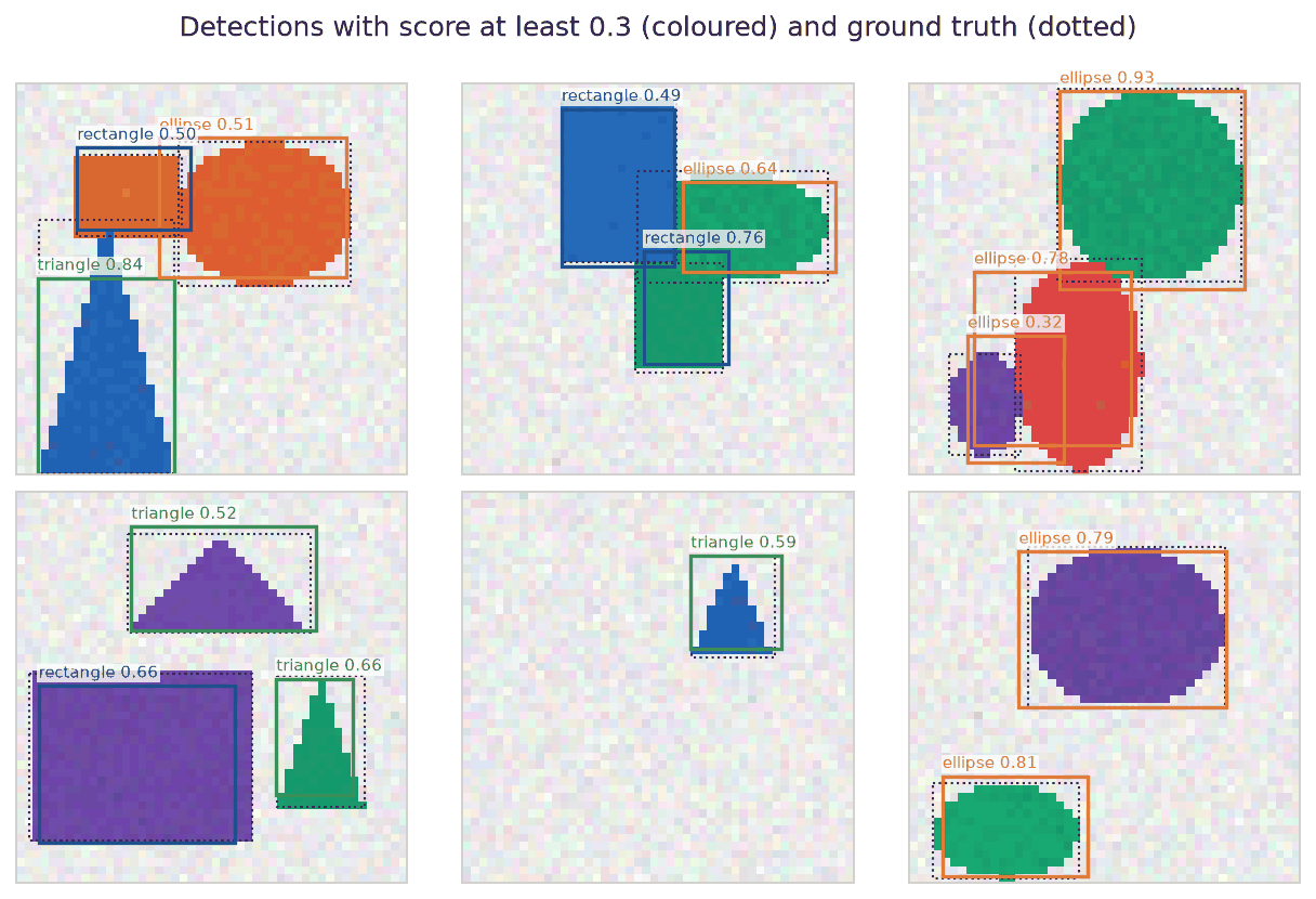
The detector finds nearly every object but places its boxes only roughly, which the drop from 0.9563 at IoU 0.5 to 0.5929 at IoU 0.75 shows and a single AP50 number would hide.

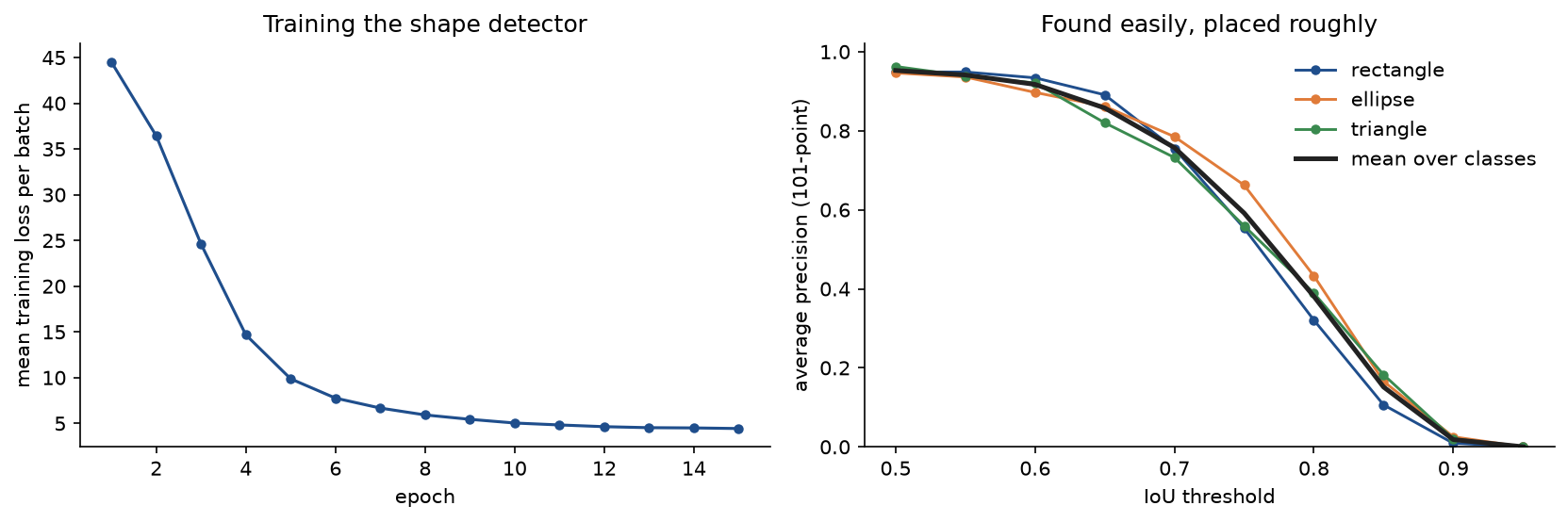
The right panel is the whole COCO-style evaluation in one picture: the left end measures whether the objects are found, the right end how precisely they are placed.

The notebook object_detection.ipynb is a guided tour in the order of this page: the overlap measures, NMS round by round, anchor matching, the grid encoding and decoding, the box regression, the tiny AP case and the simulated set, each pitfall, the shape detector and the library comparisons. The tests in tests check the worked example value by value, the mathematical properties above and the agreement with the libraries, and run in a few seconds:

python -m pytest computer-vision/object-detection

All data on this page are synthetic: simulate_detector and make_shapes generate boxes and images from a seed, so nothing is downloaded and no licence is involved.

In practice

The library functions that correspond to the package are:

• corners_to_centres and top_left_to_corners match torchvision.ops.box_convert with the formats "xyxy", "cxcywh" and "xywh", the last being the top-left form.
• box_iou, generalized_iou and distance_iou match torchvision.ops.box_iou, generalized_box_iou and distance_box_iou, and complete_box_iou adds CIoU; the losses one minus the measure are generalized_box_iou_loss, distance_box_iou_loss and complete_box_iou_loss.
• non_maximum_suppression and batched_nms match torchvision.ops.nms and torchvision.ops.batched_nms.
• encode_deltas, decode_deltas and match_anchors match the box coder and the Matcher inside torchvision's Faster R-CNN and RetinaNet.
• evaluate and coco_average_precision match pycocotools (COCOeval) and torchmetrics.detection.MeanAveragePrecision, which wraps a COCO evaluator.

torchvision and pycocotools are not part of this handbook's dependency groups, so the agreement checks here use the libraries that are. PyTorch's autograd, applied to the same overlap formulas written with tensors, reproduces the NumPy loss values exactly on 20 random box pairs, and its gradients agree with central differences of the NumPy functions to 1.5 × 10⁻¹⁰:

from object_detection import compare_overlap_losses

value_gap, gradient_gap = compare_overlap_losses(pairs=20, seed=3)
print(f"{value_gap:.1e} {gradient_gap:.1e}")

scikit-learn's average_precision_score is the non-interpolated sum computed over the detections it is given. On the tiny case, where every object is eventually found, it equals our non-interpolated AP of 0.8167. On the simulated set it equals our value only after multiplication by each class's recall ceiling, the share of objects ever matched (0.8525, 0.8224 and 0.8578 for the three classes), to ten decimals.

When moving between the package and the libraries, check these conventions. torchvision expects corner boxes in absolute pixels; its nms returns indices sorted by decreasing score and removes boxes with IoU strictly greater than the threshold, like non_maximum_suppression. COCO annotation files store top-left boxes, and its evaluator uses 101 recall points, ten IoU thresholds, at most 100 detections per image, and the annotated object area rather than the box area for the small, medium and large split.

When to use which:

• Use the from-scratch functions to learn the definitions, to reproduce a number by hand, and to debug a detector whose outputs look plausible but score badly: printing nms_rounds or the matching of the detections usually shows the problem.
• Use torchvision's operators inside a model. They run batched on accelerators, batched_nms avoids the Python loop over classes, and the IoU losses are differentiable.
• Report results with the evaluator of the benchmark you compare against, pycocotools for COCO-style numbers, and state which AP definition and which IoU thresholds the numbers use.

Running a trained detector on a phone or another device adds its own coordinate pitfalls, letterboxing and rotated camera frames among them, which the edge AI part of this handbook takes up.

Pitfalls

• Inverting the suppression rule. NMS removes the boxes whose IoU with the kept box is greater than the threshold. Some written descriptions say to discard the boxes with IoU at most the threshold, which keeps exactly the duplicates and removes the other objects. On the worked example the inverted rule returns A, B and F, three boxes on the first car and none on the second (examples/common_mistakes.py, nms_with_inverted_rule).
• Suppressing across classes. Class-agnostic NMS removes the person D in the worked example, because its box overlaps the car A with IoU 0.6672. Run NMS per class unless the classes cannot overlap in space (examples/suppress_duplicates.py).
• Mixing box formats. A COCO box (x1, y1, bw, bh) read as corners is still a valid box, just the wrong one: box A becomes (1, 2, 6, 4), a 5 by 2 box with IoU 0.4167 against the real A, and nothing raises an error. A centre-form box read as corners often has x2 below x1; the package raises ValueError for such boxes rather than returning a number. Convert at the boundary of your code and keep one format inside it.
• The extra pixel. The PASCAL VOC evaluation code and several older detection libraries measure widths as x2 - x1 + 1, treating coordinates as inclusive pixel indices. For boxes A and B that gives an IoU of 0.2353 instead of 0.1765; at twenty times the size the two conventions differ only in the third decimal, 0.1796 against 0.1765. Small objects are the most affected, and mixing the conventions between training and evaluation shifts every IoU (iou_plus_one).
• Encoding without the inverse sigmoid. If the decoder computes σ(tx) + cx, the target must be the logit of the offset, or the network must be trained so that σ(tx) matches the offset. Writing the target as the plain offset, as some descriptions do, places a perfectly trained prediction elsewhere: for the worked example the decoded centre moves from (75, 50) to (82.7232, 52.3850), almost 8 pixels to the right (decode_plain_offsets). The round trip from box to targets and back is the test that catches it (tests/test_decoding.py).
• Swapping width and height in the regression targets. The size targets are ln(gw / pw) and ln(gh / ph), width over width and height over height, and the shifts are divided by pw and ph respectively. A typo found in written versions of the R-CNN formulas divides the target width by the proposal height and vice versa. With the correct decoder, the swapped targets of the worked example decode to a 28.5714 by 98 box whose IoU with the target is 0.4000, worse than the 0.6393 of the uncorrected proposal. The mistake is invisible for square proposals, which is why it survives tests on square anchors (tests/test_pitfalls.py).
• An IoU loss for boxes that do not touch. One minus IoU is 1 with a zero gradient for every disjoint pair, so a prediction that starts away from its target never moves. For the predicted box (12, 2, 15, 6) next to box A, autograd gives a gradient of exactly zero for the IoU loss and (0.0714, -0.0268, -0.0255, 0.0268) with respect to the four corners for the GIoU loss (examples/compare_with_libraries.py, and the sliding-box plot under Worked example).
• Computing recall from the wrong denominator. Recall divides by all ground-truth boxes, including those never detected. Dividing by the number of matched objects makes every class reach recall 1 and raises the simulated set's all-point mAP at IoU 0.5 from 0.8022 to 0.9501 (map_with_recall_from_matched_objects).
• Thresholding scores before evaluation. AP is computed from the whole ranked list. Dropping the detections that score below 0.6 before evaluating cuts the curve short and lowers the simulated set's all-point mAP from 0.8022 to 0.7038; in general it can only lower it (map_after_score_threshold). A deployment threshold is chosen after evaluation, from the precision-recall curve.
• Using a ranking metric as detection AP. scikit-learn's average_precision_score on the true-positive flags knows nothing about the objects that were never detected and reports a mean of 0.9486 over the simulated set's classes, against a detection mAP of 0.8022; it also skips the interpolation (examples/compare_with_libraries.py).
• Comparing APs computed differently. On the tiny case the 11-point, all-point and 101-point APs are 0.8485, 0.8333 and 0.8350, and the COCO-style AP is 0.4380; on the simulated set the order of the first two is reversed, 0.7785 against 0.8022, and the COCO-style AP is 0.3862. A difference of a few points between two papers can be nothing but a difference of definition. The matching rule also varies: the VOC code compares a detection only with its single best-overlapping ground-truth box and calls it a false positive if that box is taken, where COCO and the package look for the best box still free.

Further reading

• R. Girshick, J. Donahue, T. Darrell and J. Malik, "Rich feature hierarchies for accurate object detection and semantic segmentation", CVPR 2014. R-CNN, with the box-regression parameterization in its appendix.
• R. Girshick, "Fast R-CNN", ICCV 2015. RoI pooling and the multi-task loss with smooth L1.
• S. Ren, K. He, R. Girshick and J. Sun, "Faster R-CNN: Towards real-time object detection with region proposal networks", NeurIPS 2015. Anchors and the region proposal network.
• K. He, G. Gkioxari, P. Dollar and R. Girshick, "Mask R-CNN", ICCV 2017. RoIAlign and instance masks.
• J. R. R. Uijlings, K. E. A. van de Sande, T. Gevers and A. W. M. Smeulders, "Selective search for object recognition", International Journal of Computer Vision 104, 154-171, 2013.
• J. Redmon, S. Divvala, R. Girshick and A. Farhadi, "You only look once: Unified, real-time object detection", CVPR 2016.
• J. Redmon and A. Farhadi, "YOLO9000: Better, faster, stronger", CVPR 2017. k-means anchors and the sigmoid offsets used on this page.
• W. Liu et al., "SSD: Single shot multibox detector", ECCV 2016.
• T.-Y. Lin, P. Goyal, R. Girshick, K. He and P. Dollar, "Focal loss for dense object detection", ICCV 2017. RetinaNet.
• T.-Y. Lin, P. Dollar, R. Girshick, K. He, B. Hariharan and S. Belongie, "Feature pyramid networks for object detection", CVPR 2017.
• N. Bodla, B. Singh, R. Chellappa and L. S. Davis, "Soft-NMS: Improving object detection with one line of code", ICCV 2017.
• H. Rezatofighi, N. Tsoi, J. Gwak, A. Sadeghian, I. Reid and S. Savarese, "Generalized intersection over union: A metric and a loss for bounding box regression", CVPR 2019.
• Z. Zheng, P. Wang, W. Liu, J. Li, R. Ye and D. Ren, "Distance-IoU loss: Faster and better learning for bounding box regression", AAAI 2020. DIoU and CIoU.
• Z. Tian, C. Shen, H. Chen and T. He, "FCOS: Fully convolutional one-stage object detection", ICCV 2019.
• X. Zhou, D. Wang and P. Krahenbuhl, "Objects as points", arXiv:1904.07850, 2019. CenterNet.
• N. Carion, F. Massa, G. Synnaeve, N. Usunier, A. Kirillov and S. Zagoruyko, "End-to-end object detection with transformers", ECCV 2020. DETR.
• M. Everingham, L. Van Gool, C. K. I. Williams, J. Winn and A. Zisserman, "The PASCAL Visual Object Classes (VOC) challenge", International Journal of Computer Vision 88, 303-338, 2010. The 11-point AP and the matching rule.
• T.-Y. Lin et al., "Microsoft COCO: Common objects in context", ECCV 2014. The COCO benchmark and its AP.
• R. Padilla, W. L. Passos, T. L. B. Dias, S. L. Netto and E. A. B. da Silva, "A comparative analysis of object detection metrics with a companion open-source toolkit", Electronics 10(3), 279, 2021. How the published AP definitions differ in practice.
• Evaluation metrics in this handbook treats precision, recall and ranking metrics for classification, the starting point of detection AP.