Q-learning¶

An agent that learns by trial and error has to find out which action is best in each situation without being told, from rewards that may arrive many steps after the decision that earned them. Q-learning keeps a table with one number per state and action, an estimate of the return from taking that action and acting optimally afterwards, and after every step corrects one entry using only the reward just received and its own estimate for the next state. It needs no model of the environment, and it learns the optimal values even while it behaves exploratorily. This page derives the Bellman optimality equation, computes the exact optimal table of a small maze by value iteration, works the first eleven Q-learning updates on that maze by hand, and trains until the learned table matches the exact one to four decimals. It then covers exploration, the learning rate and the discount factor, compares Q-learning with SARSA on a cliff, checks the cliff against Gymnasium, and states the conditions under which the method provably converges. Afterwards you will be able to carry out Q-learning on paper, implement it in a few lines, train an agent on any grid world you can draw as a text map, and tell a converged table from one that only looks finished. It builds on Markov decision processes.

To run the code in this topic, install the base group, and the rl group for the comparison with Gymnasium.

Intuition¶

Picture the agent standing in a maze with a notebook that has one line per cell and one column per direction. Each entry is the agent's current guess of how much reward it will collect if it takes that direction from that cell and plays well from then on. At first every entry is zero. After each move the agent looks at what happened, the reward it got and the cell it landed in, and asks: if my guesses for the new cell were right, what should the entry I just used have been? The answer is the reward plus the best guess in the new cell, discounted a little because it lies one step in the future. The agent moves its old guess part of the way towards that answer and walks on.

Two features make this work. The correction uses a guess to improve a guess, so information about a distant reward spreads backwards through the table one step at a time; in the hand-worked example below, the reward of the side exit reaches the start cell only in the second episode. And the correction always uses the best entry of the new cell, whatever the agent actually does next, so the table converges to the values of the best behaviour even while the agent wanders around to explore. This is what off-policy means.

The agent-environment loop: inside the agent the table Q feeds the row of the current state to an epsilon-greedy choice of action; the action goes to the environment, which returns a reward and the next state to the update step, and the update writes a new entry back into the table

The diagram shows one turn of the loop. The agent reads the row of its current state, picks an action, receives a reward and the next state from the environment, corrects one entry, and the next state becomes the current one. Nothing else is stored: no model of the maze, no list of past episodes.

How it works¶

Notation¶

The formula images write the time step as a subscript and the next state and action with a prime. In the text these are written plainly: s, a and r for the state, action and reward of one step, s' and a' for the next state and action, Q*(s, a) for the optimal value of action a in state s, and Q(s, ·) for the whole row of state s.

S and A are the finite sets of states and actions, and |A| is the number of actions.
P(s' | s, a) is the probability that action a in state s leads to state s', and r(s, a) is the expected reward of that action.
γ is the discount factor, between 0 and 1, and G is the return, the discounted sum of the rewards that follow a step.
π(a | s) is a policy, the probability of choosing a in state s, with action values Q^π and state values V^π.
Q and V are the optimal action and state values, and Q is the table being learned.
α is the step size, also called the learning rate, δ the temporal-difference error and ε the exploration probability of the epsilon-greedy policy.
The largest absolute entry of a table, the maximum over all s and a of |Q(s, a)|, is written with double bars and an infinity subscript.

States, actions, rewards and returns¶

At each step the agent observes the state s, chooses an action a, and the environment answers with a reward r and a next state s' drawn from P(· | s, a). The Markov property says that this distribution depends on the current state and action only, not on how the agent got there. An episode ends when the agent enters a terminal state, and nothing happens after that, so every value of a terminal state is zero. The return is the discounted sum of the rewards that follow:

The return at step t is r t plus 1 plus gamma times r t plus 2 plus gamma squared times r t plus 3 and so on, the sum over k of gamma to the k times r t plus k plus 1, which equals r t plus 1 plus gamma times the return at step t plus 1

With γ below 1 the sum stays finite even in tasks that never end, a reward k steps away counts γ to the power k as much as one received now, and 1 / (1 - γ) acts as an effective horizon: 20 steps for γ = 0.95. In an episodic task that is certain to end, γ = 1 is allowed. The action value of a policy is its expected return after a given first action, and the state value averages the action values over the policy's choices:

The action value of policy pi is the expected return given the state s and the first action a; the state value is the sum over actions of pi of a given s times the action value

Markov decision processes treats these definitions in full, together with the Bellman expectation equations and policy evaluation. This page needs only the optimal versions.

The Bellman optimality equation for Q¶

The optimal action value Q(s, a) is the best expected return available after taking a in s. Split the return into the first reward and the rest, as in the last form of the return above. The first reward has expectation r(s, a) whatever happens later. From the next state s' the best that can be done is V(s'), the largest entry of Q*(s', ·), and averaging over the next state gives

The optimal value of action a in state s is the expected reward plus gamma times the sum over next states of their probability times the best optimal value in that state

with the maximum taken as zero when s' is terminal. This is the Bellman optimality equation for Q. Once Q* is known, any policy that picks the best action in every state is optimal:

The optimal state value is the largest optimal action value, and an optimal policy picks an action that attains it

Choosing that action needs no model of the environment, which is the reason to learn action values rather than state values: V* alone would still require P and r to compare actions. Write the right-hand side of the optimality equation as an operator T that turns one table into another. The equation then says that the optimal table is a fixed point of T:

The operator T maps a table Q to the table whose entry for s and a is the expected reward plus gamma times the expected best entry of the next state; the optimal table satisfies Q star equals T Q star

Learning Q* therefore means finding the one table that T leaves unchanged. With the model in hand this can be done by applying T over and over; without it, by applying a sampled version of T one entry at a time, which is what Q-learning does.

Value iteration and why it converges¶

Value iteration starts from any table, usually zeros, and applies the operator repeatedly, so the table after k + 1 sweeps is T applied to the table after k sweeps. It converges because T is a contraction in the largest-entry norm. First, for any two rows of numbers, the maxima differ by at most the largest entrywise difference. Suppose the first row has the larger maximum and let a1 attain it. Then

The difference between the two maxima is at most Q1 minus Q2 at the action a1, which is at most the largest entrywise difference between Q1 and Q2

and the other case is symmetric. Second, the rewards cancel in the difference of two backed-up tables, and the next-state probabilities sum to one, so

The difference between T Q1 and T Q2 at any entry is at most gamma times the probability-weighted largest difference, which is gamma times the largest difference between Q1 and Q2

For γ below 1 the Banach fixed-point theorem then gives a unique fixed point and geometric convergence from any start:

The distance from the table after k sweeps to the optimum equals the distance between T applied to the previous table and T applied to the optimum, which is at most gamma times the previous distance, and so at most gamma to the k times the initial distance

The same inequality gives a test that does not need Q. Insert TQ between Q and Q, use the triangle inequality and the contraction, and collect the two distances to Q* on one side:

The distance from Q to the optimum is at most the distance from Q to T Q plus gamma times the distance from Q to the optimum; therefore it is at most the distance from T Q to Q divided by 1 minus gamma

The distance from TQ to Q is the Bellman residual, the largest amount by which any entry violates the optimality equation. A residual of ρ certifies that the table is within ρ / (1 - γ) of the optimum, 20 times ρ for γ = 0.95.

The temporal-difference idea¶

Value iteration needs P and r to compute the expectation inside T. An agent that only interacts with the environment does not have them, but every step hands it one sample (s, a, r, s'), and the sample target

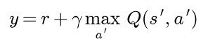
The sample target y is the reward plus gamma times the best entry of the next state

has expectation (TQ)(s, a) under the next-state distribution. The remaining question is how to average such samples one at a time. The mean of n numbers can be updated as each one arrives:

The mean of n numbers equals the mean of the first n minus 1 plus the difference between the new number and that mean, divided by n

Replacing 1 / n by a step size α gives the general rule "move the estimate a fraction α of the way towards the new sample". Applied to the sample target it becomes

Q of s, a moves by alpha times delta, where the temporal-difference error delta is the reward plus gamma times the best entry of the next state minus Q of s, a

The difference δ is the temporal-difference error: two estimates of the same quantity, made one step apart, disagree by δ. The target contains an estimate, which is called bootstrapping. Compared with waiting until the end of the episode and using the actual return, as Monte Carlo methods do, temporal-difference updates happen after every step and use a target with far less variance, at the price of a bias while the table is still wrong.

The data flow of one update: the row of the next state and the terminal flag give the bootstrap value, the reward and gamma times the bootstrap give the target, the target minus the old entry gives the TD error, and the old entry plus alpha times the TD error gives the new entry

The diagram follows one update from its inputs to the new entry. The terminal flag is the one detail that is easy to get wrong: when the next state ends the episode, the bootstrap is zero, whatever the row of that state holds.

The Q-learning update¶

Putting the pieces together, Q-learning applies after every step

$Q of s t, a t moves towards r t plus 1 plus gamma times the maximum over a prime of Q of s t plus 1, a prime, by a fraction alpha of the difference$

dropping the maximum when the next state is terminal. One episode runs as follows.

Set s to the start state.
Choose an action a, for example epsilon-greedily from the row Q(s, ·).
Take it and observe the reward r and the next state s'.
Update Q(s, a) with the rule above.
If s' is terminal, stop; otherwise set s to s' and go back to step 2.

The target uses the best next action whatever action the agent takes next, so the behaviour that generates the data does not enter the target. Q-learning is off-policy: it learns Q from any behaviour that keeps trying every action in every state. Two consequences are worth checking against the update. In a deterministic environment Q is a fixed point: if every entry already equals Q, the target equals Q(s, a) exactly and δ = 0. And with α = 1 in a deterministic environment the update replaces an entry by its target, which is value iteration applied to one entry at a time.

SARSA, the on-policy relative¶

SARSA, named after the five quantities s, a, r, s' and a' it uses, bootstraps from the action actually taken next:

Q of s t, a t moves towards r t plus 1 plus gamma times Q of the next state and the next action actually taken

It is on-policy: it learns the value of the policy it follows, exploration included. With a constant epsilon-greedy policy derived from its own table, its fixed point solves the Bellman equation with the maximum replaced by the epsilon-greedy average of the next row:

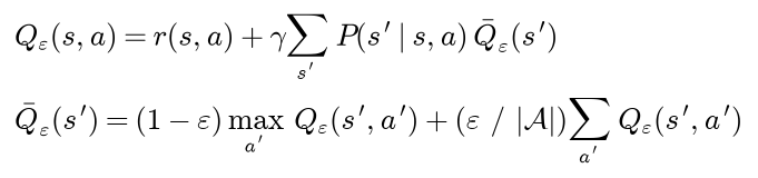
Q epsilon of s, a is the expected reward plus gamma times the expected epsilon-greedy average of the next state, which is 1 minus epsilon times the best entry plus epsilon over the number of actions times the sum of all entries

The average is the expected value of the next entry when the next action is chosen epsilon-greedily; ties for the maximum share the greedy probability, which does not change the value. It is a convex combination of the maximum and the mean of a row, and both are non-expansive, so this operator is also a γ-contraction and value iteration solves it. Expected SARSA uses this average itself as its target. If ε is decreased to zero while every action keeps being tried, SARSA converges to Q* as well.

From state s and action a the agent reaches s prime; Q-learning's target always uses the best entry of s prime, SARSA's uses the entry of whichever action its epsilon-greedy choice picks

The diagram puts the two targets side by side. They agree whenever the agent's next action happens to be the greedy one and differ only on exploratory steps, which is exactly where the cliff example below separates them.

Exploration with epsilon-greedy¶

The epsilon-greedy policy picks an action uniformly at random with probability ε and the greedy action otherwise. A random pick can land on the greedy action too, so with a unique greedy action

With a unique greedy action, epsilon-greedy picks it with probability 1 minus epsilon plus epsilon over the number of actions, and every other action with probability epsilon over the number of actions

and when several actions tie for the maximum they share the 1 - ε equally. Ties must be broken at random: at the start every entry is zero, and np.argmax would always return the first action. Common schedules lower ε over time, for example exponential decay to a floor after k episodes,

Epsilon after k episodes is the larger of a floor and the initial epsilon times d to the k

or linear decay, or ε = 1/k. A schedule is called greedy in the limit with infinite exploration (GLIE) when every state-action pair is still tried infinitely often while ε goes to zero; ε = 1/k is an example. GLIE is what on-policy methods such as SARSA need to end up with the optimal policy. Q-learning needs only the infinite exploration, because its target does not depend on the behaviour; how fast exploration decays then affects how much reward the agent collects while learning and how evenly the table gets updated, not where the table converges.

When Q-learning converges¶

The convergence theorem (Watkins and Dayan 1992, with general proofs by Jaakkola, Jordan and Singh 1994 and by Tsitsiklis 1994) says: for finite state and action sets, bounded rewards and γ below 1, the table converges to Q* with probability one provided every state-action pair is updated infinitely often, and the step sizes used for each pair at its first, second and later updates satisfy the Robbins-Monro conditions:

The sum over n of the step sizes of a pair diverges, while the sum of their squares converges

The first sum must diverge so that the steps are large enough in total to forget the initial value and reach any target. The second must converge so that the noise in the targets averages out. Per-pair schedules of the form below satisfy both, and ω = 1 is the running average:

The n-th step size is 1 over n to the omega, with omega greater than one half and at most 1

Undiscounted episodic tasks, such as the cliff below, need extra conditions on termination: Tsitsiklis (1994) covers the case in which every policy ends with probability one, and Yu and Bertsekas (2013) the case in which a policy that never ends collects an unboundedly negative return, as a policy that keeps walking into a wall does on the cliff. Two refinements matter in practice.

In a deterministic environment the target is not random, and any constant α in (0, 1] converges given infinitely many visits. An entry whose target has already settled closes the gap by the factor 1 - α at each update, so the error shrinks geometrically, as fast as the least-visited entry is updated.
With a constant α in a stochastic environment the table never settles. For a single entry whose targets are independent with variance σ², the update is a weighted average, and its variance v reaches a floor where one update leaves it unchanged:

The update m becomes 1 minus alpha times m plus alpha times y; the variance v satisfies v equals 1 minus alpha squared times v plus alpha squared sigma squared, so v equals alpha sigma squared over 2 minus alpha

A smaller α lowers that floor and slows learning. The running average α = 1/n removes the floor but can be extremely slow when γ is close to one; Even-Dar and Mansour (2003) show that 1/n to the power ω with ω below 1 converges much faster.

The theorem is a statement about the limit. It says nothing about how many episodes a particular table needs, which is governed by the pairs the behaviour visits least.

What the learning rate and the discount factor control¶

The step size trades speed against noise. In a deterministic environment larger is faster, up to α = 1; in a stochastic one a constant α sets the size of the remaining fluctuations, and a decaying schedule removes them. The discount factor belongs to the problem as much as to the algorithm. It sets the effective horizon and the scale of the values for rewards bounded in size by r_max:

The effective horizon is 1 over 1 minus gamma, and every action value is at most r max over 1 minus gamma in size

When rewards at different distances compete, γ decides which is preferred, and so it can change the optimal policy, as the maze shows below. It is also the contraction factor, so value iteration's worst-case error shrinks only like γ to the power k; in tasks whose episodes end quickly, termination does much of the shrinking and convergence is faster than that bound.

Worked example¶

The maze¶

The maze has four rows and four columns, cells named (row, column) from the top-left corner. Reading from the top, row 0 has three open cells and the goal G in column 3; row 1 is open, wall, open, open; row 2 is open, open, wall, open; and row 3 holds the start S in column 0, an open cell, the side exit E in column 2 and an open cell. Entering G ends the episode with reward +12, entering E ends it with reward +3, and every other move has reward -1, including a move into a wall or off the edge, which leaves the agent where it was. The four actions are up, right, down and left, numbered 0 to 3 in that order as in Gymnasium's grid worlds.

The discount factor is γ = 0.95 and the step size α = 0.4. Twelve cells are not terminal, so the table has 48 entries that matter; the rows of G and E stay zero. Every value is computed in double precision and shown with four decimals.

Exact values by value iteration¶

Starting from zeros, the first sweep gives every entry its immediate reward: 12 for the two moves into G, 3 for the two moves into E and -1 for everything else. From the second sweep on, values spread outwards. In sweep 2, moving right from (0, 1) is worth -1 + 0.95 × 12 = 10.4, and moving right from the start is worth -1 + 0.95 × 3 = 1.85, because E is two moves away. In sweep 3, (0, 0) learns -1 + 0.95 × 10.4 = 8.88, while (1, 0), which has not yet heard from either exit, is at -1 + 0.95 × (-1.95) = -2.8525. The state values, the best entry of each row, listed row by row from the top with the walls and exits skipped:

After sweep 1: -1, -1, 12; -1, -1, 12; -1, -1, -1; -1, 3, 3.
After sweep 2: -1.95, 10.4, 12; -1.95, 10.4, 12; -1.95, 1.85, 10.4; 1.85, 3, 3.
After sweep 3: 8.88, 10.4, 12; -2.8525, 10.4, 12; 0.7575, 1.85, 10.4; 1.85, 3, 8.88.
Final: 8.88, 10.4, 12; 7.4360, 10.4, 12; 6.0642, 4.7610, 10.4; 4.7610, 3.5229, 8.88.

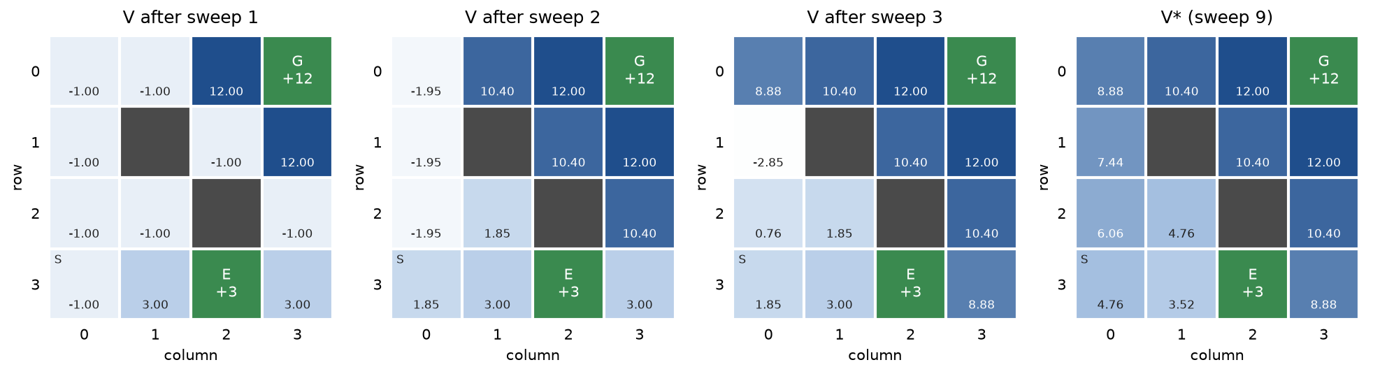
Four copies of the maze shaded by state value: after sweep 1 only the cells next to an exit carry their reward, after sweeps 2 and 3 the values spread one cell further per sweep, and the final panel shows the optimal values from 3.52 at cell (3, 1) to 12 next to the goal

The figure shows the values spreading outwards from the two exits one cell per sweep. The cell (3, 1) keeps the value 3 of its move into E until sweep 7, when the route to G finally reaches it and its value rises to 3.5229. The state values are final after sweep 7, every entry of Q after sweep 8, and sweep 9 changes nothing, so value iteration stops with the exact optimal table. The largest change per sweep was 12, 11.4, 10.83, 10.2885, 9.7741, 5.0414, 2.7654, 0.4968 and 0. The finite count is a property of deterministic mazes: exact values move one cell per sweep, and the longest optimal route, from (3, 1), is seven moves.

The values have a closed form that confirms the table. A cell k moves from an exit with reward R collects k - 1 step rewards of -1 and then R, so along that route it is worth

The value of a route of k moves to an exit with reward R is minus the sum of gamma to the j for j from 0 to k minus 2, plus gamma to the k minus 1 times R, which equals minus 1 minus gamma to the k minus 1 over 1 minus gamma plus gamma to the k minus 1 times R

The start is six moves from G and two from E, so the two routes are worth

Via G: minus 1 minus 0.95 to the 5 over 0.05 plus 0.95 to the 5 times 12, which is minus 4.5244 plus 9.2854, equals 4.7610; via E: minus 1 plus 0.95 times 3 equals 1.8500

and G wins. The full optimal table, with the rows of the two exits omitted, lists the values of up, right, down and left for each cell:

(0, 0): 7.4360, 8.8800, 6.0642, 7.4360.
(0, 1): 8.8800, 10.4000, 8.8800, 7.4360.
(0, 2): 10.4000, 12.0000, 8.8800, 8.8800.
(1, 0): 7.4360, 6.0642, 4.7610, 6.0642.
(1, 2): 10.4000, 10.4000, 8.8800, 8.8800.
(1, 3): 12.0000, 10.4000, 8.8800, 8.8800.
(2, 0): 6.0642, 3.5229, 3.5229, 4.7610.
(2, 1): 3.5229, 3.5229, 2.3468, 4.7610.
(2, 3): 10.4000, 8.8800, 7.4360, 8.8800.
(3, 0): 4.7610, 2.3468, 3.5229, 3.5229.
(3, 1): 3.5229, 3.0000, 2.3468, 3.5229.
(3, 3): 8.8800, 7.4360, 7.4360, 3.0000.

Moves into a wall or the edge are worth -1 + γ V*(s), the cost of a wasted step: moving down from the start gives -1 + 0.95 × 4.7610 = 3.5229. Two cells have two optimal actions: (1, 2), where up and right both reach G in two moves, and (3, 1), where going up or going left both begin a seven-move route to G. At (3, 1) the side exit is one move away and worth 3, yet both ways round to G are worth more, 3.5229, so at γ = 0.95 no cell should ever use E.

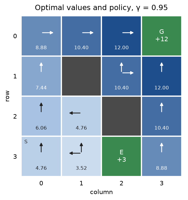
The maze coloured by the optimal state values, with an arrow for every optimal action: the start and the left column point up, the top row points right towards G, and cells (1, 2) and (3, 1) show two arrows each

The map is the optimal table in one picture: the colour and number of each cell are its value, and the arrows are the optimal policy, which never heads for E.

The first updates by hand¶

Two short episodes from an all-zero table, with α = 0.4 and γ = 0.95. The actions are a plausible random walk; the update does not depend on how they were chosen. For each step, the bootstrap is the best entry of the next state in the table as it stands before the update, taken as zero when the move ends the episode; the target is the reward plus γ times the bootstrap; the TD error is the target minus the old entry; and the new entry is the old one plus α times the TD error.

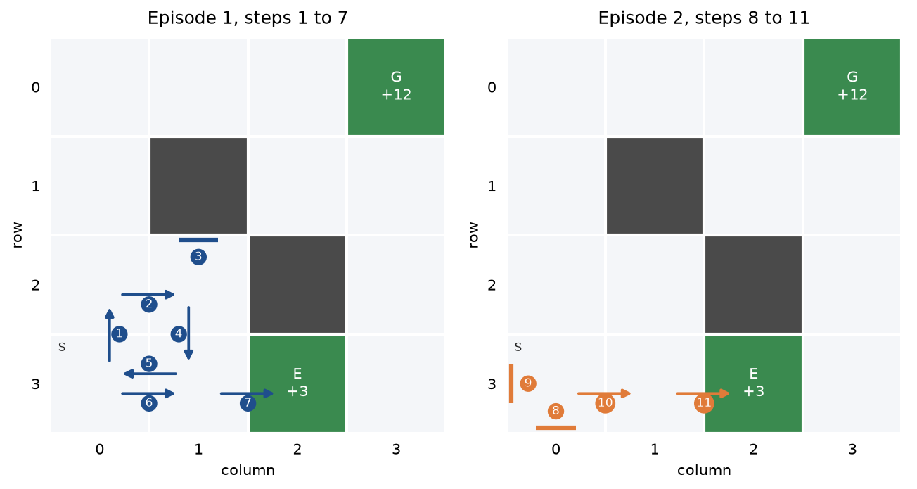
Two copies of the maze with the hand-played episodes drawn as numbered arrows: episode 1 goes up, right, bumps into the wall at step 3, comes down, steps left and right along the bottom row and enters E at step 7; episode 2 bumps into the bottom and left edges at steps 8 and 9 and then walks right into E

The figure shows where the agent went. Bumps into a wall or the edge, which leave it in place, are drawn as bars on the blocked side. Episode 1 takes up, right, up, down, left, right, right:

Step 1: from (3, 0) up to (2, 0), reward -1, bootstrap 0, target -1, TD error -1, new entry -0.4.
Step 2: from (2, 0) right to (2, 1), reward -1, bootstrap 0, target -1, TD error -1, new entry -0.4.
Step 3: from (2, 1) up into the wall, staying at (2, 1), reward -1, bootstrap 0, target -1, TD error -1, new entry -0.4.
Step 4: from (2, 1) down to (3, 1), reward -1, bootstrap 0, target -1, TD error -1, new entry -0.4.
Step 5: from (3, 1) left to (3, 0), reward -1, bootstrap 0, target -1, TD error -1, new entry -0.4.
Step 6: from (3, 0) right to (3, 1), reward -1, bootstrap 0, target -1, TD error -1, new entry -0.4.
Step 7: from (3, 1) right into E, reward +3, the episode ends, bootstrap 0, target 3, TD error 3, new entry 1.2.

Step 1 is the generic case: Q((3, 0), up) = 0 + 0.4 × (-1 + 0.95 × 0 - 0) = -0.4. In step 3 the agent bumps into the wall at (1, 1) and stays at (2, 1), so the bootstrap is the maximum of its own row, still all zeros. Step 5 is the subtle one: the row of the next state, (3, 0), is -0.4, 0, 0, 0 for up, right, down and left, and its maximum is 0, an action not yet tried. With negative step rewards, untried entries at zero look better than tried ones, which pushes a greedy agent towards actions it has not taken. Step 7 ends the episode, so there is no bootstrap and the target is the exit reward: 0.4 × 3 = 1.2.

Episode 2 starts again at (3, 0) and takes down, left, right, right:

Step 8: from (3, 0) down into the edge, staying, reward -1, bootstrap 0, target -1, TD error -1, new entry -0.4.
Step 9: from (3, 0) left into the edge, staying, reward -1, bootstrap 0, target -1, TD error -1, new entry -0.4.
Step 10: from (3, 0) right to (3, 1), reward -1, old entry -0.4, bootstrap 1.2, target 0.14, TD error 0.54, new entry -0.184.
Step 11: from (3, 1) right into E, reward +3, old entry 1.2, bootstrap 0, target 3, TD error 1.8, new entry 1.92.

Steps 8 and 9 bump into the edge; each time the row of (3, 0) still contains a zero, so the bootstrap is 0. Step 10 is the first update that uses a value learned earlier: the best entry of (3, 1) is now Q((3, 1), right) = 1.2, so

Target equals minus 1 plus 0.95 times 1.2, which is 0.14; delta equals 0.14 minus minus 0.4, which is 0.54; the new entry Q of (3, 0), right equals minus 0.4 plus 0.4 times 0.54, which is minus 0.184

The reward of E has travelled one cell backwards, from (3, 1) to the start, in one episode. Step 11 moves the exit entry again: 1.2 + 0.4 × (3 - 1.2) = 1.92. After the two episodes the rows that are no longer zero are, for up, right, down and left:

(2, 0): 0, -0.4, 0, 0.
(2, 1): -0.4, 0, -0.4, 0.
(3, 0): -0.4, -0.184, -0.4, -0.4.
(3, 1): 0, 1.92, 0, -0.4.

The agent has not seen G yet, and its table currently prefers the route to E from the start, the trap that the section on exploration returns to. An entry with a fixed target closes the gap by the factor 1 - α = 0.6 at each update. The entry for stepping from (3, 1) into E has the fixed target 3, so after n updates it holds 3 (1 - 0.6 to the power n): 1.2, 1.92, 2.352, 2.6112, 2.7667 and so on. An entry whose fixed target is the goal reward 12 needs the smallest n for which 12 × 0.6 to the power n is below 5 × 10⁻⁵, which is 25 updates. Every other entry bootstraps from entries that are themselves still moving, and cannot settle before they do.

The next decision at the start uses the row -0.4, -0.184, -0.4, -0.4. With ε = 0.2 the greedy action, right, has probability 1 - 0.2 + 0.2/4 = 0.85 and every other action 0.05. A uniform draw of 0.37 is not below 0.2, so the agent exploits and moves right; a draw of 0.13 is below 0.2, so it explores, and a second, uniform pick among the four actions chooses one, for example action 2, down. Every number in this section is asserted by tests/test_planning.py, tests/test_updates.py and tests/test_exploration.py, and printed by examples/value_iteration.py and examples/worked_updates.py.

Training until the table converges¶

To learn every entry, every state-action pair has to keep being tried. Because Q-learning is off-policy, the behaviour can be anything that does so, and the simplest choice for learning the whole table is the uniformly random policy, ε = 1. The run below starts from zeros at S, uses α = 0.4 and γ = 0.95, plays 4000 episodes with seed 0, and after each episode compares the table with the value-iteration table. The tolerance is 5 × 10⁻⁵, half a unit in the fourth decimal, the precision of every table on this page.

The greedy policy is optimal from episode 381 on.
The largest error, the largest difference between any entry and its exact value, falls below the tolerance at episode 1807, after 46,899 updates.
The residual bound, the Bellman residual divided by 1 - γ, falls below the tolerance at episode 2325.

After 4000 episodes the largest error was 8.0 × 10⁻⁹; the least visited pair had been updated 50 times and the most visited 5,751 times.

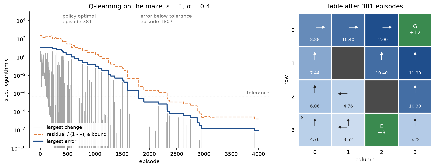
Left: largest error, residual bound and largest change per episode on a logarithmic axis over 4000 episodes, with the error falling in steps below the tolerance at episode 1807 and the bound always above it; right: the maze shaded by the table after 381 episodes, whose arrows are all optimal while the value of (3, 3) is still 5.22 instead of 8.88

The error falls in a staircase because it is set by whichever entry is currently furthest off, and that entry improves only when the random walk happens to visit it. The right panel shows the table at the moment its greedy policy became optimal for good.

How to tell when a table has converged¶

The run shows three signals that are commonly read as convergence and are not, and one that is.

The greedy policy is right long before the values are. From episode 381 on every greedy action is optimal, yet the largest error at that point is 6.4091, at (3, 3) down, a corner the random walk rarely reaches. Every arrow in the right panel agrees with the optimum while several numbers do not. A correct policy is often all that is needed, but it says little about the numbers in the table.
A small update does not mean a small error. The first episode in which no entry changed by more than 5 × 10⁻⁵ was episode 114, a two-move walk from the start into E whose two entries were already close to their targets; the largest error after it was 10.8. The grey curve in the figure, the largest change per episode, dips to tiny values throughout training.
A table that looks plausible can still break the Bellman equation. Computing the right-hand side of the optimality equation for every entry of the episode-381 table shows the culprits at once: Q((3, 3), up) = 5.2234 where the right-hand side is 8.8112, and three more entries at (3, 3) and (2, 3) whose right-hand side is 3.9622 while they hold 1.0269, 1.6632 and 2.6123.
The residual bound is a certificate. Once the residual divided by 1 - γ falls below the tolerance, the table is provably within it, without knowing Q*. Here that happened at episode 2325, later than the true error, because the bound multiplies the residual by 20. Computing the residual needs the model, or in a deterministic environment one recorded transition per state-action pair.

Without a model and in a noisy environment there is no exact certificate. Then the honest checks are: the visit count of every pair, since a pair updated a handful of times cannot be accurate whatever the rest of the table says; whether the table is stable over long windows rather than single episodes; agreement between runs with different seeds; and, for the policy, its average return measured by running it greedily for many episodes. Every number in this section is printed by examples/convergence.py and asserted by tests/test_training.py and tests/test_inspection.py.

The code¶

The package q_learning is plain NumPy, split into one module per idea. Gymnasium is imported only inside make_cliff_walking in comparisons.py, so everything else works without it.

model.py holds the array types, the Environment interface that every learner trains on, and TabularModel, the next-state probabilities, expected rewards and terminal flags of a finite environment.
gridworld.py holds GridWorld, built from rows of characters: open cells, walls, one start, cliff cells and exits, with a step reward, exit rewards, a fall reward and a slip probability of moving sideways. It steps like any environment and writes out its own tabular model.
worlds.py reads text maps: parse_map, load_map for a file or a built-in name, and maze and cliff_walk for the two worlds on this page, written in the same format as MAZE_MAP and CLIFF_MAP.
planning.py holds bellman_backup, bellman_residual, value_iteration, evaluate_policy for the exact values of a fixed policy, the error measures and route_value, the closed form above. The backup, the residual and value iteration take an optional epsilon that turns the maximum into the epsilon-greedy average of SARSA's equation.
exploration.py holds epsilon_greedy with random tie-breaking, its probabilities and policy matrix, epsilon_schedule and step_size for per-pair step sizes α / n to the power ω.
updates.py holds the Q-learning and SARSA targets, q_learning_update and sarsa_update, which return an Update record with every intermediate quantity, and replay_episode, which applies Q-learning along a given action sequence.
training.py holds train, which runs Q-learning or SARSA on any environment and returns a TrainingRun with the table, returns, episode lengths, visit counts and, given a model and a reference table, the largest and mean error, the Bellman residual and whether the greedy policy is optimal after every episode.
inspection.py reads a learned table: greedy_policy, optimal_actions, greedy_matches, first_below, settled_from, worst_entries, greedy_path and evaluate_greedy, which runs the greedy policy many times.
formatting.py prints updates, tables, value grids and policies as arrows in the layout of this page.
worked.py holds the settings and the two episodes of the worked example, and ScriptedDraws, which replays an epsilon-greedy decision with fixed random numbers.
experiments.py holds the exploration behaviours and step-size schedules compared under In practice, with runners for them; pitfalls.py holds the demonstrations for the Pitfalls section.
comparisons.py holds the bridge to Gymnasium; plotting.py and drawing.py draw every figure in the handbook's four colours.

States are numbered in reading order, skipping walls and cliff cells, and world.cell_name(state) turns a number back into (row, column). The heart of train is the update after each step:

next_state, reward, terminal = environment.step(state, action, rng)
stop_bootstrap = terminal or (truncation_is_terminal and steps == max_steps)
target = q_learning_target(q, reward, next_state, stop_bootstrap, gamma)
visits[state, action] += 1
rate = step_size(int(visits[state, action]), alpha, alpha_power)
q[state, action] += rate * (target - q[state, action])

For Q-learning the next action is chosen after the update, from the updated row; for SARSA it is chosen before, because the target needs it. The examples and the project import the package, so install the repository first as described in the main README. Each example demonstrates one idea and runs in a few seconds from the repository root:

examples/value_iteration.py computes the exact table sweep by sweep, checks it against the closed form, and compares the discount factors 0.8 and 0.95, including the number of sweeps the slippery maze needs. It saves the sweep, optimal-table and discount figures.
examples/worked_updates.py prints the eleven hand updates, repeats them in a bare NumPy loop, shows the geometric approach to a fixed target and replays two epsilon-greedy decisions. It saves the figure of the two episodes.
examples/convergence.py trains until convergence and prints the three misleading signals and the certificate. It saves the convergence figure.
examples/exploration_and_step_sizes.py compares four exploration behaviours and then constant and decaying step sizes in the deterministic and the slippery maze. It saves the exploration and step-size figures.
examples/cliff_walking.py works one cliff update by hand, solves both fixed points exactly, runs twenty learners of each kind and checks the grid against Gymnasium's CliffWalking-v1. It saves the cliff figure.
examples/common_mistakes.py demonstrates the pitfalls below: a table that only looks finished, no exploration, a time limit treated as termination, bootstrapping through a terminal state, misreading epsilon and the maximization bias.

python reinforcement-learning/q-learning/examples/value_iteration.py
python reinforcement-learning/q-learning/examples/worked_updates.py
python reinforcement-learning/q-learning/examples/convergence.py
python reinforcement-learning/q-learning/examples/exploration_and_step_sizes.py
python reinforcement-learning/q-learning/examples/cliff_walking.py
python reinforcement-learning/q-learning/examples/common_mistakes.py

The sample project¶

The sample project, project/gridworld_agent.py, is a command-line tool that trains a tabular agent on any grid world written as a text map. A map is a block of rows using . for open cells, # for walls, S for the start, C for cliff cells and any other letter for an exit, then a blank line and one setting per line: step for the reward of a move, fall for stepping into a cliff cell, slip for the chance of moving sideways and one line per exit letter with its reward. --map takes a file or the built-in names maze and cliff.

The project pipeline: a text map becomes a GridWorld; its model feeds value iteration, which gives the exact table, while its transitions feed Q-learning with a step-size schedule, a discount and an exploration schedule; the learned table and its greedy policy go to the evaluation, which also uses the exact table, and the evaluation writes the figures

The diagram shows how the pieces fit. The learner only ever sees transitions; the map also gives the full model, so value iteration supplies the exact answer to measure the learner against. The project trains with per-pair step sizes α / n to the power ω, a discount γ and ε decaying from a start value to a floor, prints progress every tenth of the run, the learned greedy policy as arrows, the learned values and the optimal policy, and then evaluates: how many pairs were never tried, in how many states the greedy action is optimal, overall and among the states the policy actually visits, the exact discounted value of the learned policy from the start against the optimum, and the share of greedy episodes ending at each exit with their mean return and length. Options such as --slip, --method, --episodes, --alpha, --alpha-power, --gamma, --epsilon-start, --epsilon-end, --epsilon-decay, --initial-value and --seed change the setup, and --figures sends the two PNGs to another folder so a custom run does not overwrite the ones shown here. The default run takes about three seconds.

python reinforcement-learning/q-learning/project/gridworld_agent.py
python reinforcement-learning/q-learning/project/gridworld_agent.py --map maze --alpha 0.4 --alpha-power 0
python reinforcement-learning/q-learning/project/gridworld_agent.py --slip 0 --initial-value 50

The default map, project/maps/shortcut.txt, has seven rows and eleven columns. A row of five traps T worth -50 lies between the start S on the left and the goal G worth +50 on the right, with a corridor on each side of the traps and a long ring round the outside; every move has reward -1 and slips sideways with probability 0.1. A corridor beside the traps is the short way, twelve moves, but each move there risks a slip into a trap, so with slipping the optimal policy takes the ring. The default run trains for 10,000 episodes with α = 1 / n to the power 0.6 per pair, γ = 0.95 and ε decaying from 1 by a factor of 0.9995 per episode to 0.05. The mean return per block of 1000 episodes climbs from -42.281 in the first block to 32.066 in the last. The evaluation reports:

8 of the 196 state-action pairs were never tried, so the largest error stays at 47.1232 from the first thousand episodes on.
The greedy action is optimal in 42 of the 49 states, and in all 17 states the greedy policy visits.
The discounted value of the learned policy from the start is 9.4227, exactly the optimum.
In 2000 greedy episodes the learned policy reached G every time, with mean return 33.036 and 17.96 moves; the optimal policy, run with the same seed, scored 33.029 and 17.97.

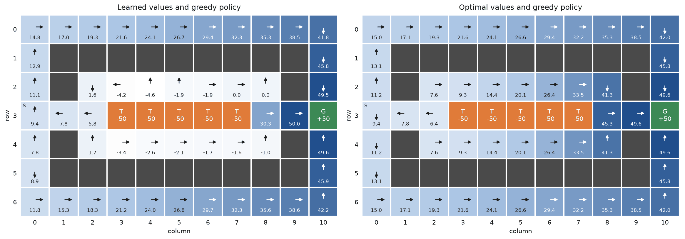
The shortcut map twice, learned and optimal, shaded by value with an arrow for each greedy action: both policies take the outer ring to G, the learned one round the top and the optimal one round the bottom, while the corridor cells next to the traps show low learned values and arrows that differ from the optimum

The learned policy goes round the top where the optimal policy goes round the bottom, two mirror-image routes of exactly the same value. Inside the ring the two maps differ: the agent learned to stay away from the traps and so never learned the corridor cells well, which costs nothing because the policy never goes there.

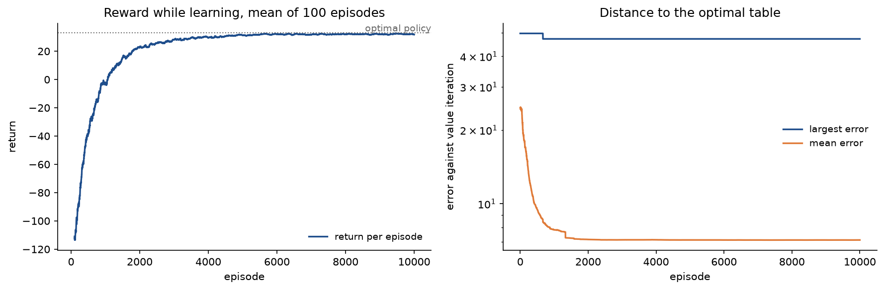
Left: the return per episode, averaged over 100 episodes, rising from about -110 to just below the optimal policy's 33; right: the largest and mean error against value iteration on a logarithmic axis, the largest error flat near 47 and the mean error falling quickly to about 7

The reward curve reaches the level of the optimal policy while the error curves stay high: the table is wrong where it does not matter and right where it does. Without slipping, --slip 0, the corridor becomes optimal and the start is worth 19.8160, but with the default schedule the agent never learns the far end of the corridor and keeps the ring, whose value from the start is 12.4304: random steps beside a row of traps rarely survive long enough to get there. Optimistic initial values fix this. With --initial-value 50 every untried action looks as good as the goal, the greedy choice keeps trying them until their entries come down, and the agent takes the corridor in 12 moves with the optimal value 19.8160.

The notebook q_learning.ipynb is a guided tour in the order of this page: value iteration on the maze, the hand-worked episodes and the same updates in bare NumPy, epsilon-greedy decisions with scripted random numbers, the training run and the convergence checks, exploration, step sizes and the discount factor, the pitfalls, the cliff comparison, the Gymnasium check and the shortcut map. The tests in tests check the worked example value by value, the contraction and residual properties, convergence, the cliff fixed points and the agreement with Gymnasium, and run in a few seconds:

python -m pytest reinforcement-learning/q-learning

Data: none is downloaded. The maze, the cliff and the shortcut map are defined in the package and in project/maps; Gymnasium's CliffWalking-v1, used for comparison, ships with Gymnasium under the MIT licence.

In practice¶

Exploration: learning the table versus earning while learning¶

Four behaviours on the maze, each for 4000 episodes with the same seed: uniformly random, a constant ε = 0.5, ε decaying from 1 by a factor of 0.99 per episode to a floor of 0.1, and pure greedy. The optimal policy collects 5 × (-1) + 12 = 7 per episode.

ε = 1: final largest error 8.0 × 10⁻⁹, greedy route to G in 6 moves, no pair left untried, mean return over the last 500 episodes -17.764.
ε = 0.5: final largest error 8.88, greedy route to G in 6 moves, 3 pairs never tried, mean return 0.404.
ε from 1 to 0.1: final largest error 12, greedy route to E in 2 moves, 16 pairs never tried, mean return 1.776.
ε = 0: final largest error 12, greedy route to E in 2 moves, 31 pairs never tried, mean return 2.000.

The side exit is a trap. From the start a random walk usually reaches E within a few moves, the table soon values the route to it at about -1 + 0.95 × 3, and an agent that explores little never travels the six moves needed to discover that G is worth more. The greedy agent earns the most while learning, 2.000 per episode, and learns the wrong policy; the random agent earns -17.764 per episode and ends with the exact table. With the decaying schedule the agent entered G only twice in 4000 episodes; the greedy agent never reached G. Only enough exploration finds G, and only exhaustive exploration fixes every entry.

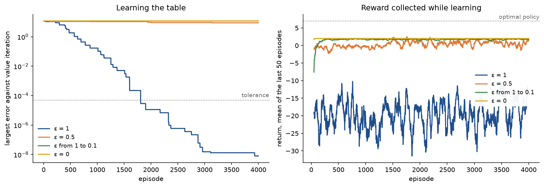
Left: largest error against value iteration over 4000 episodes for the four behaviours, only the uniformly random one falling below the tolerance while the other three stay near 9 to 12; right: the return per episode averaged over 50 episodes, the greedy and decaying behaviours flat near 2, the constant 0.5 near 0 and the random one between -30 and -10

The two panels pull in opposite directions: the behaviour that learns the table best earns the least while learning. In practice the two goals are separated where possible: explore heavily while learning, then act greedily. When reward during learning matters, decay ε slowly and keep a floor, or replace blind randomness with directed exploration, for example optimistic initial values, which make every untried action look attractive, as the sample project shows, or count-based bonuses.

Choosing the learning rate¶

With the uniformly random behaviour the episodes do not depend on the table, so runs with different step sizes see exactly the same transitions. In the deterministic maze:

α = 0.1 never brings the largest error below the tolerance; it is 0.69 after 4000 episodes.
α = 0.4 reaches the tolerance at episode 1807 and ends at 8.0 × 10⁻⁹.
α = 0.7 reaches it at episode 1013 and ends exactly at the optimum.
α = 1 reaches it at episode 391, where every entry already equals Q* in double precision.

Larger is faster here, and α = 1, asynchronous value iteration, reaches the exact table first. Noise changes the picture. In the slippery maze a move goes the intended way with probability 0.8 and sideways with probability 0.1 to each side; value iteration on its model takes 44 sweeps to reach a change below 10⁻¹², and every value drops, the start to 2.5292 from 4.7610. The largest error over all entries is dominated by the few pairs the random walk rarely reaches, so the comparison uses the mean absolute error over the 48 entries after 1000, 3000 and 10,000 episodes, again with identical episodes for every schedule:

Constant α = 0.4: 0.523, 0.308 and 0.703.
Constant α = 0.1: 0.953, 0.281 and 0.243.
Per-pair α = 1 / n to the power 0.6: 0.256, 0.118 and 0.073.
Per-pair α = 1 / n: 1.195, 0.859 and 0.594.

The constant step sizes stall at a noise floor, lower for the smaller α, and the error of α = 0.4 is larger after 10,000 episodes than after 3,000. The decaying schedule with power 0.6 keeps improving, as the Robbins-Monro conditions promise, while the running average 1/n, which also satisfies them, is the slowest of all.

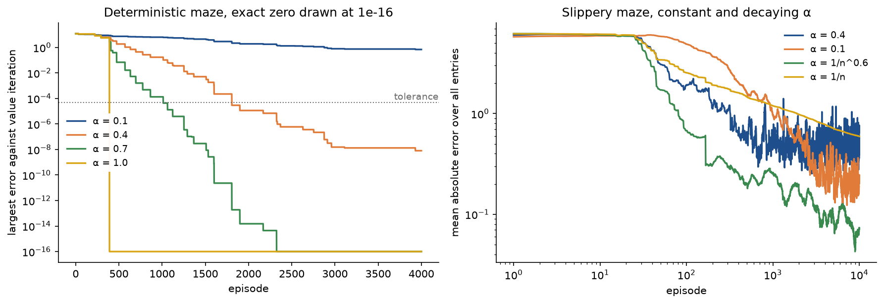
The left panel draws an exact zero at 10⁻¹⁶ so that it fits on the logarithmic axis. In a deterministic or nearly deterministic task any constant α in (0, 1] converges and a large one, up to 1, is fastest; in a noisy task, a per-pair schedule 1 / n to the power ω with ω around 0.6 to 0.8, or a constant α lowered in stages, gives both early progress and a final answer that keeps improving.

Choosing the discount factor¶

With γ = 0.8 the goal six moves from the start is worth less than the side exit two moves away: the start row becomes 0.5706, 1.4000, 0.1200 and 0.1200 for up, right, down and left, and the start, (2, 1) and (3, 1) switch to E. From the start, the two route values cross at γ ≈ 0.847.

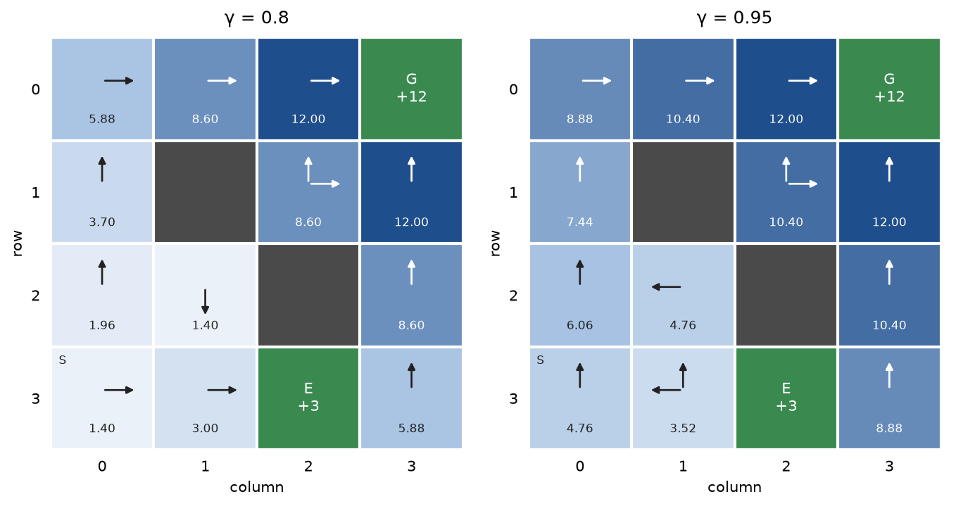
The maze shaded by optimal values for gamma 0.8 and gamma 0.95: with gamma 0.8 the bottom-left cells point right and down towards E and every value is lower, with gamma 0.95 every cell heads for G

The two maps share the shape of the maze but not the policy: a smaller discount shortens the horizon until the nearby small exit wins. The discount factor also sets the contraction rate of value iteration. In the slippery maze, value iteration needs 21, 31, 35, 39 and 46 sweeps for γ = 0.5, 0.8, 0.9, 0.95 and 0.99 to bring the largest change below 10⁻¹⁰, against 37, 115, 243, 498 and 2539 sweeps after which the worst-case bound 12 γ to the power k guarantees it. The number of sweeps grows with γ, but far more slowly than the bound, because from every cell the optimal policy reaches an exit within a few moves, so termination does most of the shrinking. Tasks without such exits, or with very long episodes, do approach the bound. Choose γ to express how far ahead the task actually looks, not as a tuning knob: a value that is too small changes the optimal policy, as above.

SARSA versus Q-learning on the cliff¶

Gymnasium's cliff-walking grid has four rows and twelve columns. The agent starts at (3, 0) and the goal is (3, 11); the ten cells between them are a cliff. Every move has reward -1, stepping into the cliff costs 100 and sends the agent back to the start, and the episode ends at the goal. The task is undiscounted, γ = 1, so Q*(s, a) is minus the number of moves to the goal, plus the penalty for any fall. Both learners use α = 0.4 and a constant ε = 0.1.

One step by hand shows where the two methods part. Start from the exact table and let the agent move right from (2, 5) to (2, 6), along the cliff edge. The row of (2, 6) holds -8, -6, -113 and -8 for up, right, down and left, where down falls into the cliff: -100 for the fall plus -13 for the walk from the start. Q-learning's target is -1 + max(-8, -6, -113, -8) = -7, exactly Q*((2, 5), right), so the TD error is 0. SARSA's target depends on the action it takes next. If the exploration draws down, which happens with probability 0.1/4 = 0.025, the target is -1 - 113 = -114, the TD error -107, and the entry drops to -7 + 0.4 × (-107) = -49.8. Averaged over SARSA's next action, with probabilities 0.925 for right and 0.025 for each other action, the target is

Minus 1 plus 0.925 times minus 6 plus 0.025 times minus 8 minus 113 minus 8 equals minus 1 minus 5.55 minus 3.225, which is minus 9.775

not -7: SARSA charges every cell next to the cliff for the falls its own exploration will cause. Each method has an exact fixed point. Q-learning's is Q, whose greedy route runs along the cliff edge in 13 moves, with value -13. SARSA's is the solution of the epsilon-greedy equation, which value_iteration(model, 1.0, epsilon=0.1) computes; its greedy route keeps one row away from the edge, along row 1, in 15 moves, and its start value is -20.7077. Evaluating the epsilon-greedy policy of each table exactly with evaluate_policy predicts the average return each learner should collect per episode while it keeps exploring: -50.8000 for epsilon-greedy behaviour on Q, where one exploratory step down from the edge is a fall, against -20.7077 for the epsilon-greedy fixed point. Twenty independent runs of 500 episodes per method:

Q-learning: mean return over the last 300 episodes -49.37, against the predicted -50.80; the greedy route after 500 episodes runs along the edge in 13 moves in all 20 runs.
SARSA: mean return -23.77, against the predicted -20.71; the greedy route takes 17 moves through the top row in 16 runs and loops forever in 4.

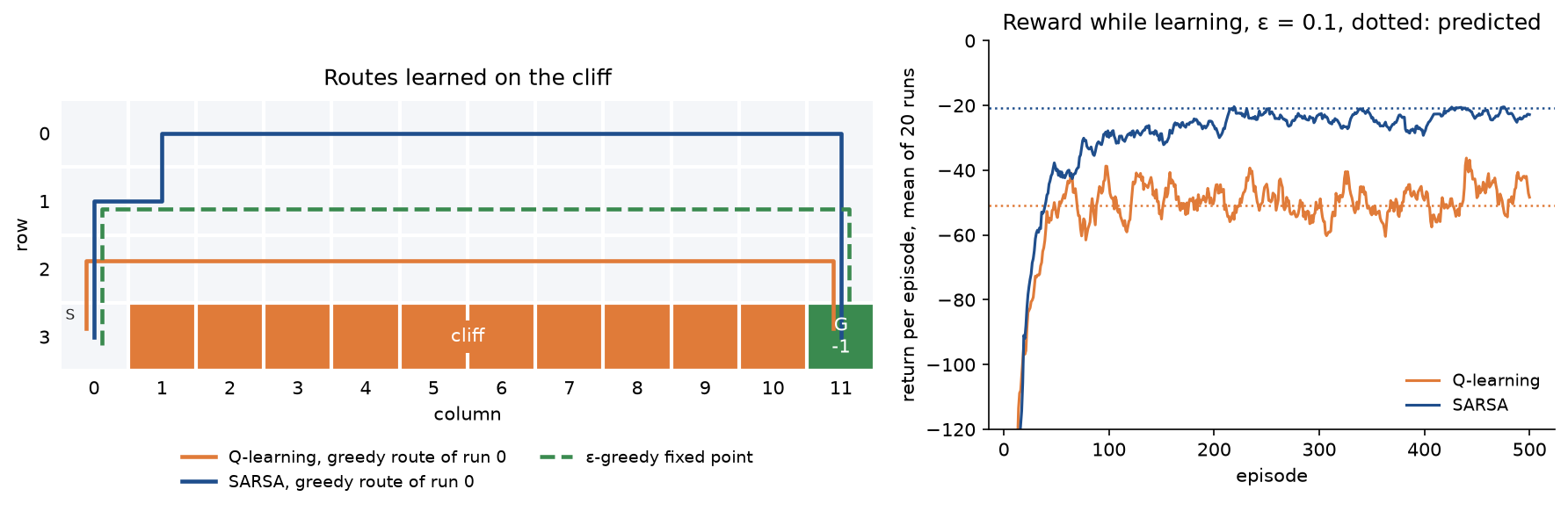
Left: the cliff grid with the greedy routes of the first run, Q-learning's along the edge in row 2, SARSA's through the top row and the epsilon-greedy fixed point along row 1; right: the return per episode averaged over 20 runs, SARSA levelling off near -23 and Q-learning near -50, each close to its dotted predicted line

Q-learning finds the optimal route and keeps falling off the cliff while it explores; SARSA collects more reward during learning and settles on a longer, safer route. With α = 0.4 its noisy estimates push it further from the edge than its exact fixed point: each of its 17-move routes climbs to the top row and spends between 5 and 12 of its cells there. In four runs SARSA's greedy route never reaches the goal: at some cell of the top row the greedy action is up, a bump into the edge, because noise has pushed its estimate just above that of the move the route needs. Which method is right depends on how the policy will be used. If exploration stops at deployment, Q-learning's route is better; if the agent keeps acting with some randomness, or mistakes are expensive while learning, SARSA's caution is worth its two to four extra moves.

The same environment in Gymnasium¶

Gymnasium supplies environments, not tabular learners; tabular Q-learning is the dozen lines of train. Its toy-text environments expose their whole transition table in env.unwrapped.P, a dictionary mapping each state and action to a list of (probability, next state, reward, terminated) tuples, which model_from_gymnasium turns into a TabularModel for value iteration:

import gymnasium as gym

from q_learning import GymnasiumEnvironment, model_from_gymnasium, train, value_iteration

env = gym.make("CliffWalking-v1")
optimum = value_iteration(model_from_gymnasium(env), gamma=1.0)
environment = GymnasiumEnvironment(env, seed=0)
run = train(environment, episodes=500, alpha=0.4, gamma=1.0, epsilon=0.1, seed=0)

examples/cliff_walking.py, the notebook and tests/test_comparisons.py check three things. The transition model of CliffWalking-v1 equals the one cliff_walk builds, entry by entry, both for the deterministic grid and for is_slippery=True, in which a move goes to the intended cell or to either side with probability one third each, our slip=2/3. Value iteration on Gymnasium's model gives the same table. And training through env.step with the same seed produces exactly the same table and returns as training on our grid, because both use the same random numbers for every decision. After 500 such episodes the table is still 3.3530 away from Q* in its worst entry although its greedy route is already the optimal 13 moves: the cliff repeats the lesson of the maze.

Gymnasium separates terminated, the episode has ended inside the task, from truncated, a time limit stopped it. Only the first may stop the bootstrap; GymnasiumEnvironment passes on terminated alone and lets train handle its own step limit. CliffWalking-v1 has no time limit by default, while FrozenLake-v1, for example, is registered with one of 100 steps.

From tables to function approximation¶

A table needs one entry per state and action and learns each entry separately, from visits to that exact pair. The maze has 48 entries, the cliff 148 and the shortcut map 196, but a robot's position measured to the centimetre, a board game or a screen of pixels has far too many states to visit each one, let alone often. The remedy is to replace the table by a parametric function with parameters θ, for example a neural network, and to move θ along the gradient of the squared difference to the same target:

The loss is the squared difference between the target y and the network's value Q of s, a with parameters theta, where y is the reward plus gamma times the network's best value in the next state

Similar states then share what is learned. The convergence theorem above does not survive this change: with function approximation, bootstrapping and off-policy updates together, the estimates can diverge. Experience replay and target networks are the measures that make it work in practice; Deep Q-networks builds them.

When to use which¶

Value iteration, when the model is known and the state space small enough to sweep: it is exact, fast, and the right way to get ground truth for testing a learner.
Q-learning, when the model is unknown and states and actions are few and discrete, and the goal is the optimal greedy policy, including learning from data collected by another policy.
SARSA or Expected SARSA, when the reward collected during learning matters, or when the agent will keep exploring after deployment and must account for its own mistakes.
Deep Q-networks or other function approximators, when the states are too many to tabulate or continuous.

Pitfalls¶

Declaring convergence too early. A greedy policy that has stopped changing, a small largest update in the latest episode and a table that looks reasonable are all compatible with large errors. In the maze run the policy was optimal at episode 381 with an error of 6.4091, and an episode with no change above 5 × 10⁻⁵ occurred at episode 114 with an error of 10.8. Check the Bellman residual of every entry and its bound when a model is available, and visit counts otherwise. examples/convergence.py and the notebook sections on training and on convergence print all of these.
Tables presented as trained that have not converged. In a deterministic task a converged table satisfies the optimality equation for every entry, so every entry for a move into an exit equals that exit's reward exactly. An exit entry equal to α times the reward has been updated once, and entries upstream that were computed from it can agree with one another and still all be wrong, because the equation fails at the exit. examples/common_mistakes.py builds such a table with frozen_exit_table: every entry except the four exit entries satisfies the equation exactly, yet the residual is 7.2 = 0.6 × 12, the largest error is 7.2, and the greedy policy heads for E from the start. Checking every entry of a printed table against the equation, or computing bellman_residual(world.model, table, gamma), takes a minute.
Too little exploration. An agent that decays ε quickly or explores not at all settles on whatever it found first. In the maze both settle on the side exit, with 16 and 31 pairs never tried and the largest error stuck at 12 (tests/test_experiments.py). On the shortcut map without slipping the default schedule keeps the ring, worth 12.4304 from the start against the optimum 19.8160, until optimistic initial values push the agent into the corridor.
A constant step size in a noisy environment. The table keeps fluctuating with a variance proportional to α and never converges; more data does not help. In the slippery maze the mean error with α = 0.4 was 0.703 after 10,000 episodes against 0.073 for α = 1 / n to the power 0.6 (examples/exploration_and_step_sizes.py).
Treating a time limit as the end of the episode. A step limit truncates the episode but the task goes on, so the last update must still bootstrap. Stopping the bootstrap there teaches the table that the world ends at the limit. With a 50-step limit in the maze, 14.5 % of random episodes were cut; bootstrapping across the cut reached a largest error of 2.3 × 10⁻⁶, stopping at it left 4.0. Starting from the exact table, a single truncated step treated as terminal moves an entry by 0.4 × (4.7610 + 1) = 2.3044 (examples/common_mistakes.py). In Gymnasium, use terminated, never terminated or truncated, to stop the bootstrap.
Bootstrapping through a terminal state. The value of a terminal state is zero by definition, not whatever its row of the table holds. With an optimistic table that starts at 20 everywhere, the target for stepping into G becomes 12 + 0.95 × 20 = 31 instead of 12 when the terminal flag is ignored, and nothing ever corrects it, because no action is taken in G (examples/common_mistakes.py).
Misreading epsilon. With ε = 0.2 and four actions the greedy action is taken with probability 0.85, not 0.8, because random picks include it. Ties for the greedy action must be broken at random: np.argmax(np.zeros(4)) is always 0, so an all-zero table would always try up first, while epsilon_greedy picks each of four tied actions about a quarter of the time.
Maximization bias. The target maximizes over noisy estimates, and the maximum of unbiased estimates is biased upwards:

The expected maximum of the estimates is at least the maximum of their expectations; for two independent standard normal variables the expected maximum is 1 over the square root of pi, about 0.5642

For two actions whose true values are both 0 and whose estimates carry independent standard normal noise, 200,000 draws give an average maximum of 0.5665 against the theoretical 0.5642. In noisy tasks Q-learning therefore overestimates, and bootstrapping passes the bias on. Double Q-learning, which selects the maximizing action with one table and evaluates it with another, removes it; the deep version appears in Deep Q-networks.

Trusting a greedy route without running it. The greedy policy of a noisy table can loop: in four of twenty cliff runs, SARSA's greedy policy bumps into the top edge forever, at (0, 5), (0, 8), (0, 2) and (0, 11). Follow the greedy policy from the start and check that it terminates before reporting a route, as greedy_path and evaluate_greedy make easy (examples/cliff_walking.py).
Comparing methods by the reward collected while learning. Q-learning looks worse than SARSA on the cliff, -49.37 against -23.77 per episode, yet its greedy route is the shorter one. Report whether a number measures behaviour during learning, with exploration, or the greedy policy afterwards, as the sample project does by evaluating the greedy policy separately.