Dimensionality reduction

Data sets with dozens or thousands of features are the rule, yet the points rarely fill the space those features span: the pixels of a handwritten digit move together, the chemical measurements of a wine are correlated, and many features are mostly noise. Dimensionality reduction finds a handful of new coordinates that keep what matters, so the data can be plotted, stored compactly, cleaned of noise and fed to models that run faster and generalize better. This page derives principal component analysis (PCA) twice, as the projection that keeps the most variance and as the one that loses the least in reconstruction, shows that both lead to the eigenvectors of the covariance matrix, computes the same answer through the singular value decomposition and explains why that route keeps more correct digits. It works a five-point example by hand, then covers explained variance and the choice of the number of components, centring and scaling, compression, whitening, the sign of a component, kernel PCA for curved structure, linear discriminant analysis as the supervised contrast, and t-SNE and UMAP for pictures. Everything is implemented from scratch in NumPy, run on the handwritten digits that ship with scikit-learn and checked against scikit-learn. Afterwards you will be able to compute principal components on paper, choose and justify the number to keep, decide whether to standardize, read a t-SNE map without over-reading it, and avoid the mistakes that make a projection lie. It builds on Linear algebra for machine learning.

To run the code in this topic, install the base and ml groups; scikit-learn, from the ml group, supplies the digits and wine data and the reference implementations.

Intuition

There are five common reasons to reduce dimensions:

• Visualization. Two or three coordinates can be plotted, and a good map shows groups and outliers. On this page 1,797 images of 64 pixels each become points in the plane.
• Compression. Fewer numbers per example, with a known reconstruction error: 20 of the 64 components keep 89 % of the digits' variance.
• Noise removal. Directions with little variance are often mostly noise, so dropping them cleans the data. Projecting noisy digits onto 15 components more than halves their error.
• Speed. Every distance, kernel and weight costs in proportion to the dimension. A nearest-neighbour classifier on 15 components is as accurate as on all 64 pixels, at a quarter of the cost per distance.
• The curse of dimensionality. In high dimension, volume hides in corners and distances concentrate, so methods built on distances lose their footing, as How it works measures and k-nearest neighbours shows for classification.

PCA is the workhorse. Picture a cloud of points shaped like a rugby ball floating in space. Its centre is the mean. Its longest axis is the direction along which the points differ most, the second longest is the longest direction perpendicular to the first, and so on. PCA moves the origin to the mean, rotates the coordinate system onto these axes and orders them by how much the cloud spreads along each. Keeping the first k axes and dropping the rest casts the cloud's shadow onto the k-dimensional plane that shows it largest. That plane is also the one closest to the points: of all planes of that dimension, the sum of squared distances from the points to it is smallest. The spread along each axis, measured as a variance, is an eigenvalue of the covariance matrix, and the direction of the axis is the matching eigenvector.

PCA is linear and ignores labels, and both limits matter. Points on two concentric circles have no straight-line projection that separates them; kernel PCA performs PCA in a feature space defined by a kernel, where the circles do come apart. And the direction of largest spread need not be the direction that separates classes; linear discriminant analysis uses the labels and looks for directions in which the classes lie far apart relative to their own spread. For pictures only, t-SNE and UMAP give up on preserving distances and try to keep each point's neighbours as neighbours, which yields much clearer maps of clusters at the cost of geometry that cannot be read literally.

The diagram is the whole page in one picture. Each method answers a different question, and none of them is finished until the result has been checked on data the method did not see, with more than one setting.

How it works

Notation

Vectors are columns, and a data matrix holds one example per row, as in NumPy and scikit-learn. There are m examples and n features. Example i is the vector x with index i, the sample mean is x̄, and the centred data matrix X has row i equal to the transposed difference between example i and the mean. The sample covariance matrix S is n by n, symmetric and positive semidefinite:

The eigenvalues of S are λ1 ≥ λ2 ≥ … ≥ λn ≥ 0 with orthonormal eigenvectors q1 to qn, so that S times qj equals λj times qj. PCA keeps k components; W is an n by k matrix with orthonormal columns, and the scores z of an example x, its coordinates along those columns, are Wᵀ(x − x̄). The thin singular value decomposition of the centred data is X = UΣVᵀ with singular values σ1 ≥ σ2 ≥ … ≥ 0. The trace of a matrix is the sum of its diagonal, and the squared Frobenius norm is the sum of its squared entries. The formula images write indices as subscripts; the text writes them plainly, as in λ1, q2 or σj. Later sections add the kernel matrix K of kernel PCA, the class means and scatter matrices of LDA, and the affinities of t-SNE, each defined where it first appears.

Why high dimension hurts

Two calculations show what goes wrong. The ball of radius 1 in d dimensions sits inside a cube of side 2. The share of the cube that the ball fills is

which is 0.7854 in the plane, 0.5236 in three dimensions, 0.00249 in ten and 2.461 × 10⁻⁸ in twenty. Uniformly spread points therefore sit almost entirely in the corners, far from the centre.

Distances also stop discriminating. Take two independent points uniform in the unit cube and let t be their difference in one coordinate. Its density falls linearly from 1 at zero to 0 at plus or minus one, and its moments follow from two short integrals:

The squared distance D between the two points is a sum of d independent copies of t squared, so its mean and variance both grow in proportion to d, and its relative spread shrinks like one over the square root of d:

At d = 2 that relative spread is 0.8367; at d = 1000 it is 0.0374. All pairwise distances crowd around the same value, so the nearest and the farthest neighbour differ little. Among 1,000 random points, the gap between the farthest and the nearest, relative to the nearest, falls from 134.6 in the plane to 0.41 in 100 dimensions and 0.12 in 1,000.

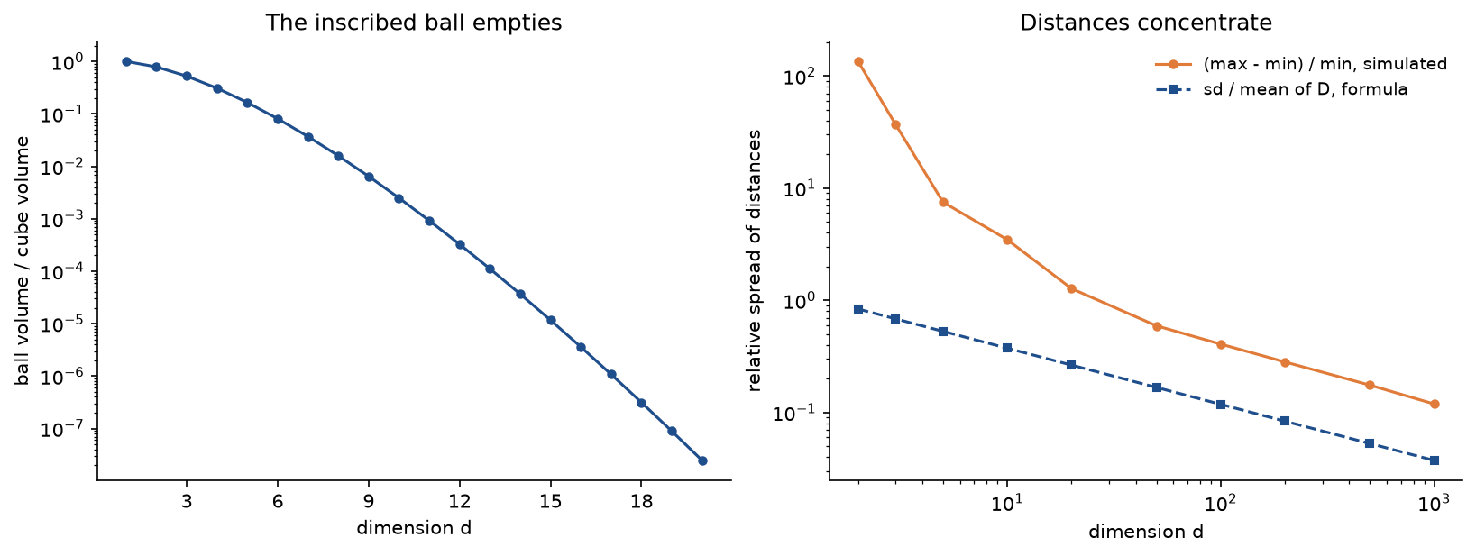
Real data escape the worst of this when they lie near a low-dimensional set, which is exactly the structure dimensionality reduction tries to find. The figure comes from examples/how_many_dimensions.py.

PCA as variance maximization

Project every centred example onto a unit vector w. The projections z are the entries of Xw. They have mean zero, because the columns of X sum to zero, and their sample variance is a quadratic form in the covariance matrix:

The first principal direction maximizes w transposed S w subject to w having unit length. With a Lagrange multiplier λ for the constraint, the gradient condition is an eigenvalue equation:

So every stationary point is a unit eigenvector, and at an eigenvector the objective equals its eigenvalue. The maximum is the largest eigenvalue λ1, reached at q1: the variance along the first principal direction is λ1.

The second direction maximizes the same objective subject to unit length and orthogonality to q1. A second multiplier γ adds a term γq1 to the gradient condition. Multiplying that condition from the left by q1 transposed, and using that q1 transposed S w equals λ1 times q1 transposed w, which is zero, leaves γ = 0, so again S w = λw. The best eigenvector orthogonal to q1 is q2, with variance λ2, and continuing in this way, the j-th principal direction is qj with variance λj.

The same result follows for all k directions at once, which also shows that choosing them jointly cannot do better. Write the total variance kept by W as a weighted sum of the eigenvalues, with weights hj that measure how much of each eigenvector W captures:

Each weight lies between 0 and 1, because W Wᵀ is an orthogonal projection and cannot lengthen the unit vector qj, and the weights add up to k, the squared Frobenius norm of Wᵀ times the orthogonal matrix of all eigenvectors. A sum of the eigenvalues with weights between 0 and 1 that add up to k is largest when weight 1 goes to the k largest eigenvalues. Any rotation of those k columns attains the maximum too, so what the optimization really determines is the subspace. If λk is strictly larger than λk+1, that subspace is unique; the individual components inside it are then fixed by asking for uncorrelated scores in order of decreasing variance. The scores along different eigenvectors are indeed uncorrelated, because qj transposed S ql equals λl times qj transposed ql, which is zero for j ≠ l.

PCA as minimum reconstruction error

Now look for the k-dimensional affine subspace closest to the data: approximate each example by a point μ plus a combination W z of k orthonormal directions, and minimize the total squared error J over μ, W and the coefficients z. For fixed μ and W, each z is a small least-squares problem whose solution is the projection, and the best μ is the mean:

The residual is then the part of the centred example that lies outside the subspace, and Pythagoras splits every centred example into the part W keeps and the part it loses. Summing over the examples turns the error into the total scatter minus the variance kept:

The first term does not depend on W, so minimizing the reconstruction error is exactly maximizing the variance kept, and the previous section solved that problem: W = [q1, …, qk], with a minimum error of m − 1 times the variance left out. The two views are one optimization written twice; the worked example traces both along every direction of a two-dimensional cloud. The same subspace is learned by a linear autoencoder trained with squared error, which is the starting point of the reconstruction-error detectors in Anomaly detection.

PCA through the singular value decomposition

The centred data have a thin singular value decomposition X = UΣVᵀ, with orthonormal columns in U and V and the singular values on the diagonal of Σ. Substituting it into the covariance matrix gives an eigen-decomposition of S directly:

The principal directions are the right singular vectors, the variances are the squared singular values divided by m − 1, and the scores of all examples are UΣ. Keeping k components reconstructs the centred data as the first k columns of U times the first k singular values times the first k rows of Vᵀ, which by the Eckart-Young theorem is the best approximation of X of rank k in the Frobenius norm. Linear algebra for machine learning derives the decomposition and that theorem.

The diagram shows both routes to the components. fit_pca takes the solid path by default and the dashed covariance route with method="eigen".

Why the SVD route is numerically preferred

Both routes are exact in exact arithmetic; they differ in what rounding does to them. A stable symmetric eigensolver returns the eigenvalues of S with absolute errors of the order of ε times λ1, where the machine epsilon ε is about 2.2 × 10⁻¹⁶, and forming XᵀX in floating point already commits errors of that size. A stable SVD of X returns singular values with absolute errors of the order of ε times σ1. For the smallest component, with the condition number κ the ratio of the largest to the smallest singular value, the relative errors are therefore:

The covariance route squares the condition number and keeps about 16 − 2 log₁₀ κ correct digits of the small variances, the SVD route about 16 − log₁₀ κ. A cloud whose variances along three axes are exactly 1, 0.25 and 10⁻¹⁸ has κ = 10⁹. The SVD finds the smallest variance with a relative error of 3.4 × 10⁻⁹, while the covariance matrix returns −5.1 × 10⁻¹⁹, a negative variance with no correct digit at all; examples/common_mistakes.py prints both.

Cost and memory point the same way when n is large: the SVD never forms the n by n covariance matrix, and when n exceeds m, the m by m Gram matrix XXᵀ or a truncated SVD is far cheaper. For tall data with many more rows than columns, the covariance route is faster and can be accumulated in chunks, and when only the leading components matter its precision is ample. scikit-learn's PCA with the default svd_solver="auto" uses it when there are at least ten times as many rows as columns and at most 1,000 columns. For a few components of a very large matrix, randomized SVD and Lanczos methods compute only the top of the spectrum.

Explained variance and choosing the number of components

The total variance is the trace of S, the sum of all eigenvalues and also the sum of the variances of the original features: PCA only redistributes it. The explained variance ratio of component j and the cumulative ratio of the first k components are

The denominator is the total variance, not the sum of the kept eigenvalues. A scree plot draws the eigenvalues against their index, often on a logarithmic axis. Five common ways to choose k:

• A variance threshold keeps the smallest k whose cumulative ratio reaches 0.9 or 0.95. It is simple and common, but the threshold is arbitrary, and a high threshold keeps noise.
• The elbow keeps the components before the scree curve flattens. It is subjective, and many spectra have no clear elbow.
• The Kaiser rule keeps the components of the correlation matrix whose eigenvalue exceeds 1, so each kept component explains more than one standardized feature. On unstandardized data it is meaningless, because the eigenvalues then carry units.
• Parallel analysis keeps the leading components whose eigenvalue beats the 95th percentile of the eigenvalues of data with every column shuffled on its own. Shuffling destroys the correlations but keeps each column's variance, so it estimates the eigenvalues that sampling noise alone produces.
• Downstream validation keeps the k that maximizes the cross-validated performance of the model that uses the components, with PCA fitted inside each training fold. When there is a task, it is the most relevant rule.

On 300 points in 20 dimensions built from three latent factors plus noise, the first three ratios are 0.5526, 0.2544 and 0.1383, together 0.9453, and every later one is below 0.005. The 90 % threshold, the Kaiser rule and parallel analysis all pick 3, but 95 % asks for 4 components and 99 % for 16, keeping pure noise.

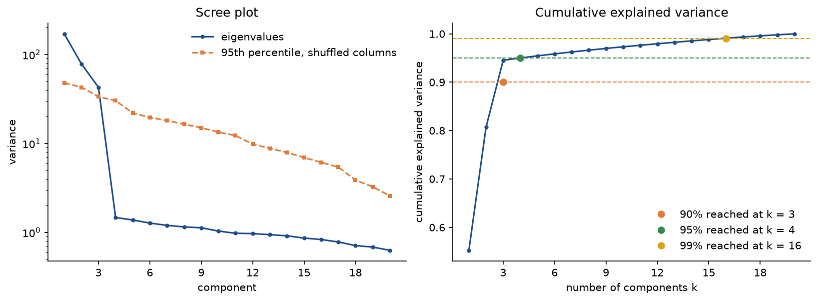
The scree plot shows three components standing clear of the noise floor, and the cumulative curve shows how far a fixed threshold can overshoot. Probabilistic PCA turns the choice into model selection; scikit-learn's n_components="mle" implements Minka's estimate.

Centring and scaling

Centring is part of the definition. The covariance matrix describes deviations from the mean, and an SVD of uncentred data describes deviations from the origin instead: when the mean is large compared with the spread, the first right singular vector of the raw data simply points at the mean. scikit-learn's TruncatedSVD deliberately skips centring, because centring would destroy the sparsity of a term-document matrix, so its first component is a mean direction.

Scaling is a choice, and it changes the answer. Measuring feature j in a unit aj times smaller multiplies column j by aj:

That is not a similarity transform unless all factors are equal, so the eigenvectors change, and a feature with a large numerical range captures the first component whether or not it matters. Standardizing every feature, subtracting its mean and dividing by its sample standard deviation sj, replaces S by the correlation matrix

whose eigenvectors do not depend on the units and whose eigenvalues add up to n. In two dimensions the correlation matrix, with ones on the diagonal and the correlation ρ off it, always has the same eigenvectors, whatever the variances were:

Standardize when features are in different units or their variances are not comparable, as for the wine measurements under Pitfalls. Do not standardize when all features share a unit and their variances carry meaning, as for pixel intensities or spectra, because standardizing inflates nearly constant features, which are mostly noise, to the same weight as the informative ones. scikit-learn's StandardScaler divides by the population standard deviation, with m in the denominator, so after it PCA reports eigenvalues m / (m − 1) times those of the correlation matrix, with identical components and ratios.

Reconstruction and compression

With k components an example is stored as its k scores and rebuilt as the mean plus W times the scores. A data set of m examples then costs mk scores, nk component entries and n numbers for the mean:

On the examples PCA was fitted on, the relative squared error is exactly the left-out share of the variance, one minus the cumulative ratio; new examples rebuild somewhat worse. PCA on blocks of pixels is the Karhunen-Loeve transform, the energy-optimal transform that the fixed discrete cosine transform of JPEG from scratch approximates without having to be fitted and transmitted. Because noise spreads its variance over all directions while signal concentrates in a few, rebuilding from a moderate number of components also removes noise.

Whitening

Whitening rescales the scores to unit variance by dividing each by the square root of its eigenvalue, with Λk the diagonal matrix of the first k eigenvalues and Q the matrix of all eigenvectors:

Any rotation of white data is white again, so whitening is not unique. ZCA whitening, short for zero-phase component analysis, rotates back with the full set of eigenvectors; of all whitening transforms it changes the data least, so whitened images still look like images. Euclidean distance after full whitening is the Mahalanobis distance of the data's covariance. Whitening divides by the square root of each eigenvalue, so components with tiny variance, often pure noise, are blown up to the same size as the strongest signal; keep only components with real variance, or add a small constant to every eigenvalue before dividing.

The sign and the uniqueness of components

If q is an eigenvector of S, so is −q, so each unit eigenvector is defined only up to sign, and its scores flip with it. Reconstructions are unaffected, because a score times its component is the same with both signs flipped. Different libraries, versions and even builds of the linear algebra library return different signs, so software fixes a convention to make its output reproducible: scikit-learn's PCA, like flip_signs here, flips each component so that its entry of largest magnitude is positive. When two entries tie in magnitude, rounding decides, as in the standardized worked example below.

When eigenvalues are equal the ambiguity is a rotation, not a sign: every orthonormal basis of the shared eigenspace is a valid set of components. When they are merely close, small changes in the data rotate the components freely within their span. Five bootstrap resamples of an isotropic Gaussian cloud put the first component at angles from 25 to 71 degrees. Only the subspace of components with nearly equal eigenvalues is meaningful, so compare such components by the angles between subspaces, and align signs, for example by the sign of a dot product with a reference, before comparing components across fits.

Kernel PCA

Kernel PCA performs PCA on φ(x), the images of the examples under a feature map φ into a space that may be infinite-dimensional, using only the kernel k(x, x′), the inner product of two mapped points. Assume for now that the mapped points are centred. Their covariance operator C has eigenvectors in the span of the mapped examples, and substituting that expansion into the eigenvalue equation and taking inner products with every mapped example turns the problem into one about the m by m kernel matrix K, whose entries are the kernel between every pair of examples:

Other solutions of the squared equation differ from these only by vectors in the null space of K, which do not change v. The feature-space vector must have unit length, which fixes the scale of the coefficients, and the projection of any point onto v then needs only kernel evaluations, with a the unit eigenvector of K:

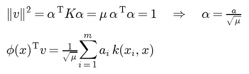
For a training point the projection simplifies to the square root of μ times its entry of a. Centring in feature space is done on the kernel matrix, with the m by m matrix whose entries are all 1/m:

A new point must be centred with the training statistics: from each of its kernel values subtract the mean of that training column, subtract the mean of its own row, and add the grand mean of the training kernel. With the linear kernel, the centred kernel matrix is XXᵀ, its eigenvalues are the squared singular values and the scores are UΣ: ordinary PCA. With the RBF kernel

the feature space is infinite-dimensional, kernel PCA can return up to m − 1 components, and the width γ decides which structure the leading components describe. The price is an m by m kernel matrix and an eigen-decomposition whose cost grows with the cube of m, and there is no exact way back to input space: the point whose image is closest to a reconstructed feature vector, the pre-image, has to be approximated.

Linear discriminant analysis

LDA uses labels. With classes c = 1 to C of sizes mc and means μc, and overall mean μ, define the within-class scatter matrix SW and the between-class scatter matrix SB:

They add up to the total scatter around the overall mean. Along a direction w the projected classes have within-class scatter wᵀ SW w and between-class scatter wᵀ SB w, and Fisher's criterion asks for classes far apart relative to their own spread. It does not depend on the length of w, and setting its gradient to zero gives a generalized eigenvalue problem:

The stationary directions are generalized eigenvectors, the value of J at each is its eigenvalue, and the best direction belongs to the largest. When SW is invertible this is the ordinary eigenproblem of SW⁻¹ SB. The C vectors that build SB, weighted by the class sizes, add up to zero, so SB has rank at most C − 1, and LDA yields at most C − 1 useful directions: one for two classes, nine for ten digits. For two classes SB always points along the difference of the class means, and the solution has a closed form:

A numerically sound solver whitens the within-class scatter first. With the eigen-decomposition of SW / (m − C), dropping eigenvalues that are numerically zero, the problem becomes an ordinary symmetric eigenproblem, and the discriminant directions are mapped back through the whitening. The projected data then have the identity as pooled within-class covariance, so Euclidean distance in LDA space is the Mahalanobis distance of the shared class covariance, and a nearest-centroid rule there is the LDA classifier for Gaussian classes with a common covariance and equal priors. Unlike principal directions, discriminant directions are not orthogonal in the input space. Where PCA keeps the directions of largest total variance, LDA keeps the directions of largest class separation; the figure under Pitfalls shows a case where the two disagree completely. LDA overfits when the number of features approaches the number of examples, and shrinking SW towards a multiple of the identity is the usual remedy.

t-SNE

t-SNE, t-distributed stochastic neighbour embedding, places points in two dimensions so that each point keeps its neighbours. It starts from similarities in the data. For point i, a Gaussian of width σi turns squared distances into conditional probabilities of picking point j as a neighbour:

The width is set separately for each point through the perplexity, two to the power of the entropy of the point's neighbour distribution in bits:

A distribution spread evenly over k neighbours has perplexity exactly k, so the perplexity is an effective number of neighbours. Entropy grows monotonically with σi, so a bisection finds the width that gives every point the same perplexity, typically between 5 and 50. Points in dense regions get small widths and points in sparse regions large ones, which is why t-SNE equalizes the apparent density of clusters. The conditional probabilities are symmetrized into joint ones,

which sum to one over all pairs and give every point a total of at least 1 / (2m), so outliers keep a say. In the map, similarities use a Student-t kernel with one degree of freedom:

The positions minimize the Kullback-Leibler divergence from P to Q:

Its asymmetry is the point. Neighbours placed far apart, with large p and small q, cost a lot, while distant points placed close, with small p and large q, cost little. t-SNE therefore protects local structure and has little incentive to get large distances right.

The gradient has a short derivation. Write w for the unnormalized Student-t weights and Z for their sum. Because the p add up to one, the cost splits into a constant, a sum over the weights and the logarithm of Z, and each pair containing i appears twice:

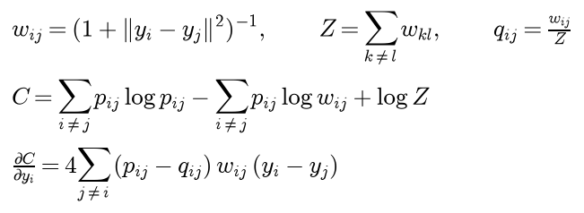
The derivative of log w with respect to yi is −2w(yi − yj), and the derivative of w itself is −2w² times the same difference; collecting the terms from the middle sum and from log Z gives the last line. Each pair acts as a spring along the line between the two points: attractive when p exceeds q, repulsive when q exceeds p.

The Student-t kernel answers the crowding problem. In ten dimensions a point can have eleven neighbours all at the same distance from one another; in the plane only three points can be mutually equidistant, and the area available at moderate distance from a point is tiny compared with the volume of the corresponding shell in high dimension. With a Gaussian kernel in the map too, moderately distant points would be squeezed together and the clusters would crush into one another. The heavy-tailed Student-t kernel lets them move far away. Ignoring the normalizations, the affinity a Gaussian assigns at distance r is assigned by the Student-t kernel at a larger distance s:

That distance is 0.8054 for r = 1, 2.5277 for r = 2 and 9.4349 for r = 3. Near neighbours stay near, moderate distances are stretched, and gaps open between clusters.

The optimization is gradient descent with momentum, 0.5 for the first 250 iterations and then 0.8, an individual adaptive gain per coordinate, and early exaggeration: for the first 250 iterations every affinity in P is multiplied by 12, which pulls clusters tight while they can still move through one another. tsne follows scikit-learn's defaults, a learning rate of the larger of m/48 and 50, and a start from the first two principal components scaled to a standard deviation of 10⁻⁴, which makes runs reproducible and preserves more of the global arrangement than a random start. The exact gradient costs time proportional to m² per iteration; the Barnes-Hut approximation computes the affinities from about three times the perplexity nearest neighbours and approximates the repulsion with a quadtree in time proportional to m log m, and interpolation with the fast Fourier transform goes further.

Reading a map

What a t-SNE map does and does not show:

• Reliable: which points are neighbours, and clusters that stay separated across perplexities and seeds.
• Not reliable: cluster sizes, because each point's width adapts to its local density; distances between clusters, which depend on the perplexity; the axes and the orientation, which are arbitrary; and apparent structure at low perplexity, where pure Gaussian noise breaks into small clumps.
• There is no mapping for new points: the map is the solution of one optimization for one set of points.

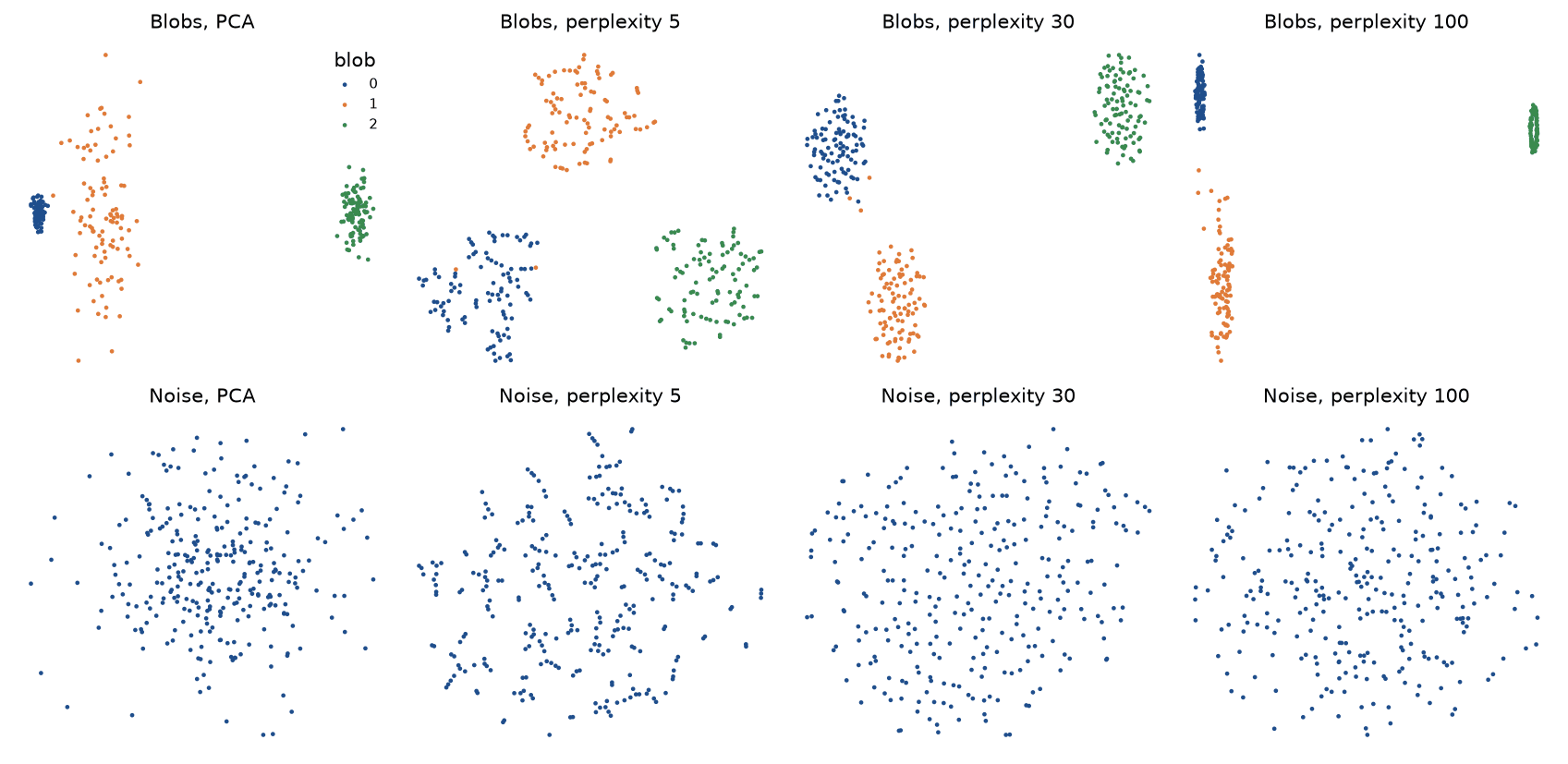
The blobs live in ten dimensions: blob 1 is five times wider than blob 0, and blob 2 is five times farther from blob 0 than blob 1 is. In the data the measured width ratio is 5.25 and the gap ratio 4.92. At perplexity 30 the map shows a width ratio of 1.20, and the gap ratio becomes 1.09, 2.87 or 9.11 at perplexities 5, 30 and 100. The bottom row is pure noise, which PCA shows as the round cloud it is and t-SNE at low perplexity tears into strands. examples/tsne_maps.py draws the figure and prints the ratios.

A map is judged by how well it preserves neighbourhoods. The trustworthiness of a map with k neighbours penalizes points that are among the k nearest neighbours of i in the map but not in the data, by how far down the data's neighbour ranking of i they are, where Ui is that set of intruders and r(i, j) the rank of j among the data neighbours of i:

A trustworthiness of 1 is perfect. The leave-one-out accuracy of the nearest point in the map, the share of points whose nearest map neighbour has the same label, adds a check of how well the classes stay apart.

UMAP

UMAP, uniform manifold approximation and projection, is not installed in the handbook's environment, so it is described here without code or tested claims. It also builds a neighbour graph and lays it out in the plane, but with different ingredients. For each point i it takes the k nearest neighbours, where n_neighbors plays the role of the perplexity, the distance ρi to the nearest one, and a scale σi chosen so that the edge weights below add up to log₂ k. Every point's nearest neighbour is fully connected, and the weights are symmetrized by a fuzzy union. In the map, the similarity is a curve with two fitted constants a and b that stays flat up to the distance min_dist, which controls how tightly points may pack:

The layout minimizes the cross-entropy between the two sets of fuzzy memberships, whose first part attracts neighbours and whose second repels non-neighbours, by stochastic gradient descent with negative sampling, starting from a spectral embedding of the graph. Compared with t-SNE it is usually faster on large data, scales to millions of points, and can place new points with transform. Its maps share t-SNE's caveats: cluster sizes and gaps are not to scale, and much of the global arrangement attributed to UMAP comes from its spectral start; t-SNE started from PCA arranges clusters comparably. In practice it is one line with the umap-learn package: umap.UMAP(n_neighbors=15, min_dist=0.1, random_state=0).fit_transform(features).

Worked example

Five points in the plane, small enough for pen and paper: (2, 2), (3, 4), (8, 4), (9, 6) and (8, 9). Every value below is computed in double precision and shown with four decimals where it is not exact.

Covariance and eigenvalues

The mean is ((2 + 3 + 8 + 9 + 8) / 5, (2 + 4 + 4 + 6 + 9) / 5) = (6, 5), and the centred points, the rows of X, are (−4, −3), (−3, −1), (2, −1), (3, 1) and (2, 4). The scatter matrix XᵀX has rows (42, 24) and (24, 28); for example, the off-diagonal entry is 12 + 3 − 2 + 3 + 8 = 24. Dividing by m − 1 = 4 gives the covariance matrix S with rows (10.5, 6) and (6, 7), whose trace, the total variance, is 17.5. The eigenvalues are the roots of the characteristic polynomial:

So λ1 = 15 and λ2 = 2.5. They add up to the trace and multiply to the determinant of S, 37.5.

Eigenvectors, in the right order

For λ1 = 15, the first row of (S − 15I)v = 0 reads −4.5v1 + 6v2 = 0, so v2 = 0.75v1 and the unit eigenvector is q1 = (4, 3) / 5 = (0.8, 0.6); the second row checks, 6 × 0.8 − 8 × 0.6 = 0. For λ2 = 2.5, the first row reads 8v1 + 6v2 = 0, which gives q2 = (−3, 4) / 5 = (−0.6, 0.8), signed so that its largest entry is positive. The two are orthogonal, 0.8 × (−0.6) + 0.6 × 0.8 = 0.

The first principal component is the eigenvector of the largest eigenvalue. np.linalg.eigh returns the eigenvalues in ascending order, (2.5, 15), so its first column belongs to λ2; the components must be sorted by eigenvalue, largest first, before they are numbered. The explained variance ratios are 15 / 17.5 = 0.8571 and 2.5 / 17.5 = 0.1429: one direction carries six sevenths of the variance.

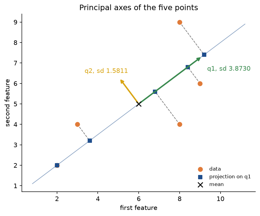
The arrows are drawn one standard deviation long, the square roots of the eigenvalues. Each dashed line is the residual a point loses when it is rebuilt from its first score alone.

Scores, reconstruction and the two views

The scores are the centred points in the new coordinates, z1 = 0.8x1 + 0.6x2 and z2 = −0.6x1 + 0.8x2 for each centred point. For point 1 they are 0.8 × (−4) + 0.6 × (−3) = −5 and −0.6 × (−4) + 0.8 × (−3) = 0. For all five points:

• The first scores are −5, −3, 1, 3 and 4, and the second scores are 0, 1, −2, −1 and 2.
• Rebuilt from the first score alone, the mean plus z1 times q1, the points become (2, 2), (3.6, 3.2), (6.8, 5.6), (8.4, 6.8) and (9.2, 7.4).
• The residuals, z2 times q2, are (0, 0), (−0.6, 0.8), (1.2, −1.6), (0.6, −0.8) and (−1.2, 1.6).

The variances of the score columns are (25 + 9 + 1 + 9 + 16) / 4 = 15 and (0 + 1 + 4 + 1 + 4) / 4 = 2.5, the eigenvalues, and their covariance is (0 − 3 − 2 − 3 + 8) / 4 = 0: the scores are uncorrelated. Point 1 lies exactly on the first axis. The squared residual lengths are 0, 1, 4, 1 and 4, a total reconstruction error of 10 = (m − 1)λ2 = 4 × 2.5, while the squared first scores add up to 60 = 4 × 15, and the two add up to the total scatter, the trace of XᵀX, 42 + 28 = 70.

That split holds for every direction, not only the best one. Sweeping a unit vector through all angles, m − 1 times the variance of the projections plus the squared reconstruction error is 70 throughout; the variance peaks at 15 and the error bottoms out at 10, both at 36.87 degrees, the angle of (0.8, 0.6).

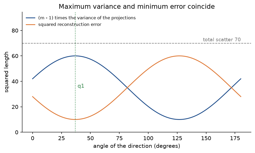
The two curves are reflections of each other in the line at 35, so maximizing one is minimizing the other: the two derivations of PCA describe one optimum.

The same through the SVD

The singular values of X are σ1 = √60 = 7.7460 and σ2 = √10 = 3.1623, so the squared singular values divided by m − 1 return the eigenvalues. The right singular vectors are q1 and q2, and the left singular vectors are the scores divided by the singular values:

• u1 = (−5, −3, 1, 3, 4) / √60 = (−0.6455, −0.3873, 0.1291, 0.3873, 0.5164).
• u2 = (0, 1, −2, −1, 2) / √10 = (0, 0.3162, −0.6325, −0.3162, 0.6325).

np.linalg.svd happens to return (0.8, 0.6) as the first right singular vector, while the eigenvector of the largest eigenvalue from np.linalg.eigh comes out as (−0.8, −0.6): equally correct, with every score negated. The sign convention turns both into (0.8, 0.6).

Whitening

Dividing the scores by √15 = 3.8730 and √2.5 = 1.5811 whitens them. The whitened points are (−1.2910, 0), (−0.7746, 0.6325), (0.2582, −1.2649), (0.7746, −0.6325) and (1.0328, 1.2649), which is √(m − 1) U = 2U and has the identity as covariance matrix. The ZCA matrix, the inverse square root of S, adds up the two eigenvector outer products divided by the square roots of their eigenvalues; it has rows (0.3929, −0.1796) and (−0.1796, 0.4977). It maps the first centred point (−4, −3), which lies on the first axis, to (−1.0328, −0.7746): the same direction, shrunk by 1/√15. PCA whitening sends the same point to (−1.2910, 0), coordinates along the principal axes; ZCA stays in the original axes.

Standardization and units

The standard deviations of the two features are √10.5 = 3.2404 and √7 = 2.6458, and their correlation is ρ = 6 / √73.5 = 0.6999. Standardized PCA therefore has eigenvalues 1 + ρ = 1.6999 and 1 − ρ = 0.3001, a first ratio of 0.8499, and components (0.7071, 0.7071) and (0.7071, −0.7071). The first direction moved from 36.87 to 45 degrees, and the second component's entries tie in magnitude, so the sign convention falls back on rounding: (−0.7071, 0.7071) is just as valid.

Now record the second feature in a unit ten times smaller, multiplying its column by 10. The covariance matrix gets rows (10.5, 60) and (60, 700), and its determinant is 100 × 37.5 = 3750:

The first component is (0.0861, 0.9963), almost the second axis, and it explains 0.9925 of the variance. Nothing about the points changed except a unit. Standardized PCA gives (0.7071, 0.7071) again in the new unit, because the correlation matrix does not see units.

Skipping the centring is the other classic slip. The first right singular vector of the raw points is (0.7728, 0.6346), close to the direction of the mean, (6, 5) / √61 = (0.7682, 0.6402), rather than q1. Move the same cloud so that its mean is (−12, 16) and the uncentred direction becomes (−0.6, 0.8), the minor axis.

t-SNE affinities by hand

Take one point with three neighbours at distances 1, 2 and 3, so the squared distances are 1, 4 and 9. With σ = 1 the Gaussian weights, e to the minus half the squared distance, are 0.6065, 0.1353 and 0.0111, which sum to 0.7530. Dividing by the sum:

• With σ = 1 the probabilities are (0.8055, 0.1797, 0.0148), the entropy is 0.7861 bits and the perplexity 2 to that power, 1.7244.
• With σ = 2 the weights are 0.8825, 0.6065 and 0.3247, the probabilities (0.4866, 0.3344, 0.1790), the entropy 1.4784 bits and the perplexity 2.7864.

As σ grows the perplexity approaches 3, the number of neighbours, and as σ shrinks it approaches 1. Bisection for a target perplexity of 2, one bit of entropy, finds σ = 1.1555 and the probabilities (0.7272, 0.2365, 0.0364). In the map the same three distances would get Student-t weights 1 / (1 + d²) of 0.5, 0.2 and 0.1 against Gaussian weights of 0.6065, 0.1353 and 0.0111: at distance 3 the Student-t kernel is nine times heavier, which is what lets t-SNE push moderately distant points away.

Every number in this section is printed by examples/worked_example.py and asserted by tests/test_trace.py and tests/test_affinities.py.

The code

The package dimensionality_reduction is plain NumPy, split into one module per idea. scikit-learn is imported only inside the functions that load its data sets or compare with it, so everything else works without it.

• arrays.py holds the Array type, as_data, which insists on one example per row, centring, the covariance and correlation matrices and all pairwise squared distances.
• eigen.py holds sorted_eigh, which puts the largest eigenvalue first, and the sign conventions flip_signs and align_signs.
• pca.py is the heart of the topic: the frozen PCAModel with transform, inverse_transform and reconstruct, components stored as rows as in scikit-learn, and fit_pca with the SVD and covariance routes, standardization and whitening.
• selection.py holds the rules for choosing k, components_for_variance, kaiser_count and parallel_analysis, and the reconstruction errors and storage counts.
• trace.py holds the worked example: trace_pca keeps every intermediate value, format_pca_trace prints them, and direction_sweep computes the variance and error along every direction.
• kernel_pca.py holds the kernels, the centring of training and test kernels, and fit_kernel_pca.
• lda.py holds the scatter matrices, fit_lda with the whitening solver, and Fisher's criterion for any direction.
• affinities.py holds the t-SNE affinities: Gaussian rows, perplexity, the bisection calibrate_row, the joint and Student-t affinities, the KL divergence and the worked perplexity trace.
• tsne.py holds the t-SNE cost, its gradient and the optimizer tsne.
• neighbours.py holds trustworthiness, neighbourhood overlap, leave-one-out accuracy, nearest-neighbour and nearest-centroid classifiers, and cluster widths and gaps.
• high_dimensions.py holds the ball fraction, the spread of distances and the relative contrast.
• datasets.py generates every synthetic data set from a seed and loads the digits and the wine data.
• experiments.py holds the small studies the examples, the project and the notebook share: accuracy on k components, denoising, compression, map quality and blob ratios.
• pitfalls.py holds deliberately wrong code for the Pitfalls section.
• comparisons.py runs every method's scikit-learn counterpart and measures the differences.
• plotting.py, pca_plots.py and image_plots.py draw every figure in the handbook's colours and save it reproducibly.

Python counts from zero, so components[0] is the first principal direction q1, stored as a row. The heart of fit_pca is a few lines in either route, followed by the sign convention:

if method == "svd":
    _, singular_values, vt = np.linalg.svd(prepared, full_matrices=False)
    variances = singular_values**2 / (count - 1)
    components = vt
elif method == "eigen":
    values, vectors = sorted_eigh(prepared.T @ prepared / (count - 1))
    variances = values[:limit]
    components = vectors[:, :limit].T

total_variance is computed from the prepared data, the squared Frobenius norm of X over m − 1, so the ratios of a truncated model are still shares of the whole. The t-SNE gradient is the formula derived above, written with the matrix of coupling strengths (p − q) times w:

q, weights = student_t_affinities(y)
coupling = (np.asarray(p, dtype=np.float64) - q) * weights
return 4.0 * (coupling.sum(axis=1)[:, None] * y - coupling @ y)

The examples and the project import the package, so install the repository first as described in the main README. Each example demonstrates one idea and runs in a few seconds from the repository root:

• examples/worked_example.py prints every value of the worked example in the order above, the sweep over directions and the perplexity by hand, and saves the two worked-example figures.
• examples/how_many_dimensions.py measures the curse of dimensionality and tries the rules for choosing k on the planted data, saving the two figures shown under How it works.
• examples/kernel_pca_and_lda.py unrolls the concentric circles with kernel PCA across five widths, compares PCA and LDA on two elongated classes and lets LDA overfit pure noise.
• examples/tsne_maps.py checks the calibrated affinities and the gradient, then maps the unequal blobs and pure noise at three perplexities.
• examples/common_mistakes.py demonstrates every mistake under Pitfalls and saves the wine scaling figure.
• examples/compare_with_sklearn.py measures the agreement with scikit-learn quoted under In practice.

python machine-learning/dimensionality-reduction/examples/worked_example.py
python machine-learning/dimensionality-reduction/examples/how_many_dimensions.py
python machine-learning/dimensionality-reduction/examples/kernel_pca_and_lda.py
python machine-learning/dimensionality-reduction/examples/tsne_maps.py
python machine-learning/dimensionality-reduction/examples/common_mistakes.py
python machine-learning/dimensionality-reduction/examples/compare_with_sklearn.py

The sample project

The sample project, project/digits_explorer.py, explores the 1,797 handwritten digits with every method of the topic in three stages. It first describes the data with PCA on all images: how the variance is spread, what the components look like and what compression costs. It then checks on held-out images what a reduction keeps: a stratified split puts 450 images aside, PCA and LDA are fitted on the other 1,347 only, noisy test images are denoised by projection, and a 1-nearest-neighbour classifier runs on k components, on LDA's nine discriminants and on the raw pixels. Finally it draws PCA, LDA and t-SNE maps of all images and scores how faithfully each keeps the neighbourhoods. Options such as --seed, --noise, --perplexity, --iterations and --tsne-per-digit change the setup, and --figures sends the five PNGs to another folder so a custom run does not overwrite the ones shown here. The default run takes well under a minute, most of it in the exact t-SNE of all 1,797 images.

python machine-learning/dimensionality-reduction/project/digits_explorer.py
python machine-learning/dimensionality-reduction/project/digits_explorer.py --tsne-per-digit 60 --perplexity 10

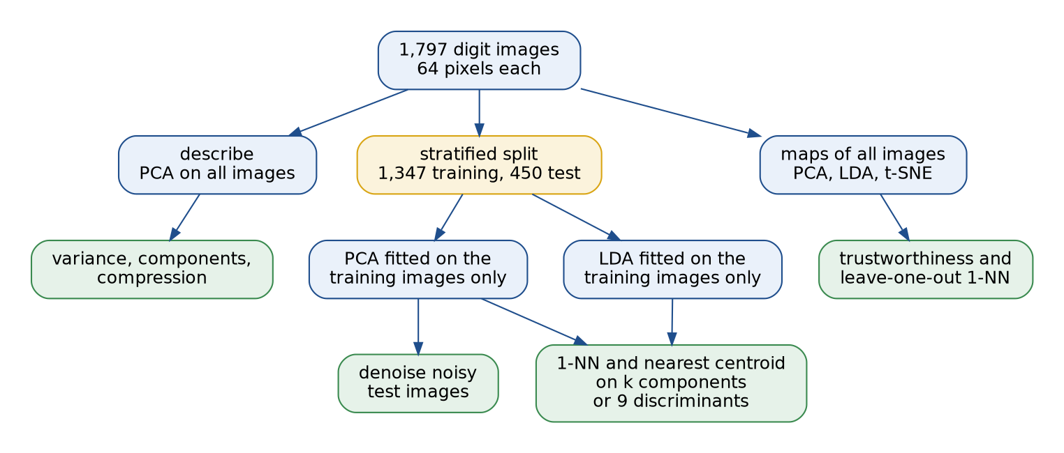
The split matters for the middle branch only: describing the data and drawing maps of it evaluate nothing, while denoising and classification are measured on images the fitted model never saw.

Three pixels are zero in every image, so at most 61 components carry variance. The pixels share one unit, so PCA runs on raw intensities. The first five components explain 0.1489, 0.1362, 0.1179, 0.0841 and 0.0578 of the variance, the first two together 0.2851. Reaching 50 %, 80 %, 90 %, 95 % and 99 % takes 5, 13, 21, 29 and 41 components. The rules for k disagree, as they usually do on real data: the Kaiser rule on the correlation matrix keeps 17 components and parallel analysis 9, the point where the eigenvalues sink below those of the shuffled data.

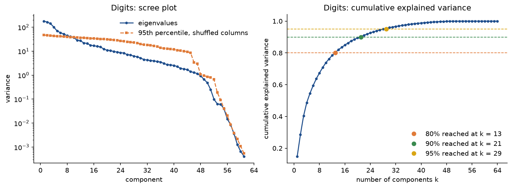
There is no elbow and no clean threshold, which is the usual situation: the number to keep depends on what the components are for.

The components read as images: each is a pattern of pixels that brighten (orange) and darken (blue) together in proportion to its score. The first ones contrast whole strokes; later ones add finer, more local detail.

Compression follows the storage formula. Ten components store 18,674 numbers instead of 115,008, 16 % of the original, with a relative squared error of 0.2618; twenty store 32 % with an error of 0.1057; forty store 65 % with an error of 0.0118. On the fitted images each error equals the left-out share of the variance.

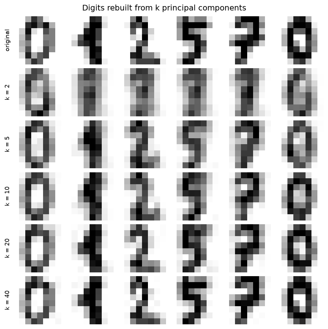
Two components keep the rough mass of the image, ten keep the strokes, and forty are hard to tell from the original.

Denoising works because noise spreads over all 64 directions while the digits concentrate in a few. With Gaussian noise of standard deviation 4 added to every pixel, the noisy test images have a mean squared error of 15.6797 against the clean ones. Projecting them onto the components of the noisy training images brings it to 7.6663 with 10 components and 7.1551 with 15, the best value; beyond that the extra components bring back more noise than signal, 7.3513 at 20 and 10.5513 at 40, and all 64 return the noisy images unchanged.

Fewer dimensions also feed a classifier. With PCA fitted on the training images and a 1-nearest-neighbour classifier on the scores, the test accuracy is 0.6044 with 2 components, 0.9022 with 5, 0.9778 with 10 and 0.9867 with 15, against 0.9822 on all 64 pixels: the same accuracy, or slightly better, with every distance costing a quarter as much. LDA with its nine discriminants reaches 0.9644 with a nearest-centroid rule against 0.8956 for nine principal components, because its directions are chosen to separate the digits; with a 1-nearest-neighbour rule the nine principal components do better, 0.9800 against 0.9622, since nearest neighbours profit from the detail that LDA throws away.

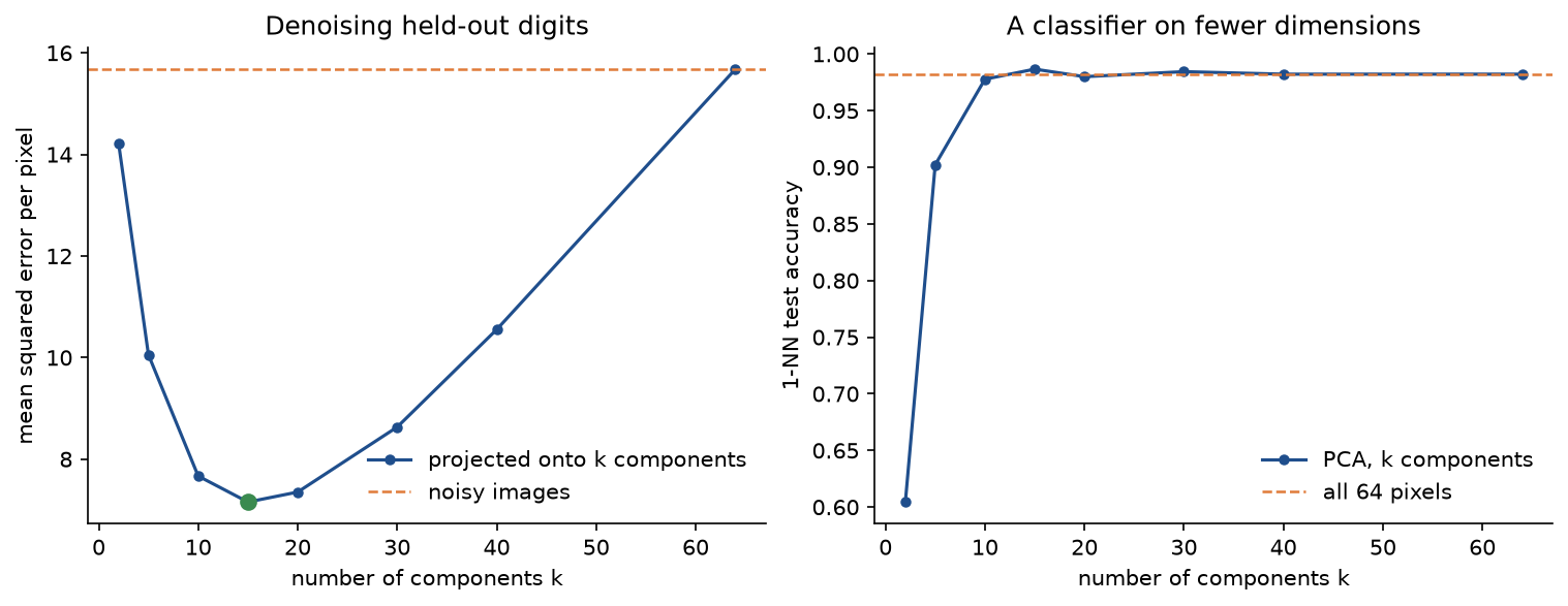
The left curve has a clear optimum and the right one a clear knee, both near 15 components: chosen by the task, k is no longer arbitrary.

PCA, LDA and t-SNE give very different pictures of the same images. Measured with ten neighbours, and with the leave-one-out accuracy of the nearest point in the map:

• PCA with 2 components: trustworthiness 0.8300, leave-one-out accuracy 0.5871.
• LDA with 2 discriminants: trustworthiness 0.7991, leave-one-out accuracy 0.6149. LDA was fitted with the labels it is scored on, so this number flatters it.
• t-SNE at perplexity 30, from scratch on all 1,797 images: trustworthiness 0.9927, leave-one-out accuracy 0.9883, final divergence 0.6825.

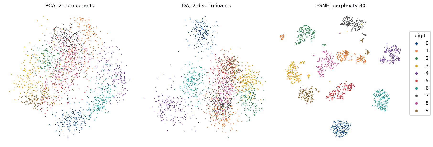
Two linear dimensions keep only 28 % of the variance, and the digits overlap. t-SNE keeps neighbourhoods almost perfectly, and nearly every image's nearest neighbour in the map is the same digit. Its small satellite groups, such as a handful of ones far from the main group of ones, are a reminder that apparent sub-clusters need checking in the original space before they are given a meaning.

The notebook dimensionality_reduction.ipynb is a guided tour in the order of this page: the curse of dimensionality, the worked example through trace_pca and again in bare NumPy, the two views of PCA, the numerical accuracy of both routes, choosing k, scaling, whitening, kernel PCA, LDA, t-SNE from perplexity by hand to maps of blobs and noise, each pitfall, the digits and the comparison with scikit-learn. It limits the linear algebra library to one thread, so its numbers are reproducible; on other processors they may differ in the last digits. The tests in tests check the worked example value by value, the mathematical properties above, the digit numbers quoted here and the agreement with scikit-learn, and run in a few seconds:

python -m pytest machine-learning/dimensionality-reduction

Data: the handwritten digits are the test portion of the Optical Recognition of Handwritten Digits data of E. Alpaydin and C. Kaynak (1998) from the UCI Machine Learning Repository, 1,797 images of 8 by 8 pixels with intensities from 0 to 16, which scikit-learn ships as sklearn.datasets.load_digits. The wine data are the Wine data of the UCI Machine Learning Repository, chemical analyses of 178 wines from three cultivars by M. Forina and colleagues, shipped as sklearn.datasets.load_wine. Both are licensed under Creative Commons Attribution 4.0, and nothing is downloaded. Every other data set is synthetic and generated from a fixed seed.

In practice

Production code uses scikit-learn, whose estimators compute the same quantities:

from sklearn.decomposition import PCA

from dimensionality_reduction import fit_pca, load_digit_images

images, _ = load_digit_images()
ours = fit_pca(images, 10)
theirs = PCA(10, svd_solver="full").fit(images)
print(abs(ours.components - theirs.components_).max())

examples/compare_with_sklearn.py runs every comparison. The largest absolute differences it measures are:

• fit_pca against PCA(svd_solver="full") on the digits: components 5.0 × 10⁻¹⁴ on the 61 informative components, signs included; variances 3.7 × 10⁻¹³; ratios 3.6 × 10⁻¹⁶; scores 5.0 × 10⁻¹³.
• fit_pca(method="eigen") against PCA(svd_solver="covariance_eigh"): components 1.7 × 10⁻¹⁴.
• fit_pca(whiten=True) against PCA(whiten=True): scores 3.9 × 10⁻¹⁴ and inverse transform 5.0 × 10⁻¹⁴.
• fit_pca(standardize=True) against StandardScaler followed by PCA: components 2.6 × 10⁻¹⁴, and variances 2.0 × 10⁻¹⁴ after the factor m / (m − 1).
• fit_kernel_pca against KernelPCA(kernel="rbf") on the circles: eigenvalues 1.1 × 10⁻¹⁴ and projections of new points 4.2 × 10⁻¹⁵.
• fit_lda against LinearDiscriminantAnalysis() on the digits: scores 7.3 × 10⁻¹² up to sign and the factor √((m − C) / m), ratios 2.0 × 10⁻¹⁵.
• joint_probabilities against the affinities inside TSNE: a relative difference of 6.4 × 10⁻⁵, because scikit-learn's bisection runs in single precision.

The three pixels with zero variance make the last three components an arbitrary basis of a null space, which is why the PCA comparison covers the 61 informative components. The LDA factor is a normalization choice: fit_lda gives the discriminant scores unit pooled within-class variance with the unbiased divisor m − C, while scikit-learn's default solver divides by m.

t-SNE is not convex, the two implementations differ in floating-point details, and scikit-learn uses the Barnes-Hut approximation by default, so coordinates cannot be compared. On three Gaussian blobs, where scikit-learn's exact method applies, the divergence it reports for its layout, 0.3297, equals the divergence tsne_cost computes for the same layout, which confirms that the two minimize the same objective. On 600 digits, 60 of each, the layouts agree in every way that matters. Measured with our affinities, our layout reaches a divergence of 0.4492 and scikit-learn's 0.4667, while its own Barnes-Hut estimate is 0.5308. The trustworthiness is 0.9883 against 0.9863, the leave-one-out accuracy 0.9683 against 0.9667, and on average 0.9125 of each image's ten nearest neighbours in one map are among its ten nearest in the other. trustworthiness and sklearn.manifold.trustworthiness agree exactly on data without tied distances; the digits have integer pixels and therefore ties, and the two then differ in the sixth decimal, 0.988259 against 0.988260, because they break ties differently.

When to use which:

• PCA for compression, denoising, decorrelation and as a preprocessing step inside a pipeline. Use the SVD (svd_solver="full") when small components matter, a randomized solver for a few components of large data, IncrementalPCA for data that do not fit in memory, and TruncatedSVD for sparse matrices that must not be centred.
• Kernel PCA when the structure is curved and the data set has at most a few thousand points; choose the kernel width by the downstream task.
• LDA as a supervised projection for classification with few classes, with shrinkage when the features are many; it doubles as a classifier.
• t-SNE and UMAP for pictures only. Try several perplexities or neighbour counts and seeds, start from PCA, and never cluster, classify or measure distances on the map instead of the data.
• Other methods worth knowing: factor analysis and probabilistic PCA, which model the noise of each feature; independent component analysis, which finds statistically independent rather than merely uncorrelated components; non-negative matrix factorization, which finds parts-based components for counts and intensities and also drives recommender systems; random projections, which preserve distances approximately by the Johnson-Lindenstrauss lemma with no fitting at all; Isomap and locally linear embedding for manifold learning; and autoencoders, the non-linear generalization of PCA.

Pitfalls

• Taking the wrong eigenvector. np.linalg.eigh sorts eigenvalues in ascending order, so vectors[:, 0] is the eigenvector of the smallest eigenvalue, the minor component. On the worked example it projects onto (0.6, −0.8), whose scores have variance 2.5 instead of 15; plotted as "the first principal component", it is perpendicular to the cloud's long axis. np.linalg.eig does not sort at all, and both return eigenvectors as columns, so vectors[0], a row, mixes components. Sort by eigenvalue, largest first, and take columns; np.linalg.svd returns Vᵀ with the components as rows, in decreasing order. examples/common_mistakes.py prints the wrong column and its variance.
• Forgetting to centre. The SVD of raw data finds directions from the origin. On the worked example the first direction is (0.7728, 0.6346), the direction of the mean, and with the cloud moved to mean (−12, 16) it is the minor axis (−0.6, 0.8). examples/common_mistakes.py prints all three directions.
• Scaling, or not, without thinking. On the wine data, proline has a standard deviation of 314.9 while most features have about 1, so raw PCA's first component is proline alone, with weight 0.9998, explaining 0.9981 of the variance. Standardized, the first component spreads over all features and explains 0.3620, and the two-dimensional map separates the cultivars with a leave-one-out 1-NN accuracy of 0.9494 instead of 0.7191. Conversely, standardizing pixels or spectra inflates nearly constant features into noise of full weight. examples/common_mistakes.py prints the numbers and draws the figure.

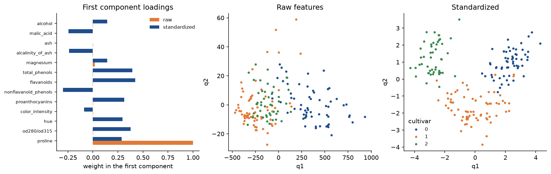
One feature in large units decides the raw analysis on its own; standardized, every measurement has a say and the cultivars come apart.

• Explained variance over the kept components. The ratio divides by the total variance. Ten components of the digits explain 0.1489, 0.1362, 0.1179 and so on, 0.7382 in all; dividing by the kept sum instead reports 0.2017, 0.1845, 0.1598 and a total of exactly 1, whatever is kept. examples/common_mistakes.py prints both.
• Choosing k by a fixed threshold alone. On the planted three-factor data 95 % asks for 4 components and 99 % for 16, where 3 are signal. Look at the scree plot, run parallel analysis, and when there is a task, validate k on it, as the project does for denoising and classification.
• Fitting PCA before the train-test split. PCA uses no labels, yet components fitted on rows that include the test rows bend towards them, and the test set then looks easier than new data. With 30 components and 100 training and 100 test digits, the held-out reconstruction error per pixel is 0.5957 when PCA saw all rows and 1.2127 when it saw only the training rows; with 1,000 and 797 images the gap shrinks to 0.7802 against 0.8514 but persists. Fit PCA inside the pipeline, on each training fold. examples/common_mistakes.py prints three sizes, and Data leakage and pitfalls measures the effect on classification scores.
• Reading meaning into signs, or into components with similar eigenvalues. A component and its negation are equally correct, and solvers disagree: on the worked example eigh returns (−0.8, −0.6) and svd returns (0.8, 0.6). When eigenvalues are close, the components rotate freely within their span: bootstrap resamples of an isotropic cloud put the first component anywhere between 25 and 71 degrees. Align signs before comparing fits, and interpret only subspaces whose eigenvalues are well separated from the rest. examples/common_mistakes.py prints the solvers' signs and the five angles.
• Whitening every component. Whitening gives each kept component unit variance, including components that hold only noise. Four pixels are zero in all 1,347 training digits, so the last four of their 64 components carry only rounding error, with variances near 10⁻³⁰. Whitened with all 64 components, a 1-nearest-neighbour classifier falls to 0.4978; whitened with 40 it scores 0.9756 and with 20 it scores 0.9822, against 0.9800 unwhitened, as examples/common_mistakes.py prints.
• Trusting the covariance route for small components. Forming XᵀX squares the condition number. On the ill-conditioned cloud the smallest variance comes out negative from the covariance matrix and correct to eight digits from the SVD. It does not matter for the leading components of well-conditioned data, which is why scikit-learn uses the covariance route for tall data by default, but it matters for nearly collinear features and for anything that uses the smallest components, such as whitening or detecting collinearity. examples/common_mistakes.py prints both estimates.
• Expecting PCA to keep what separates the classes. Two classes stretched along one axis and separated along the other, low-variance one: the first principal component is the stretch, with a Fisher ratio of 0.0009, and a classifier on it scores 0.54, while the first discriminant has a Fisher ratio of 3.4035 and scores 0.97. Unsupervised reduction before a classifier can discard the signal; validate it, or use a supervised method. examples/kernel_pca_and_lda.py prints both.

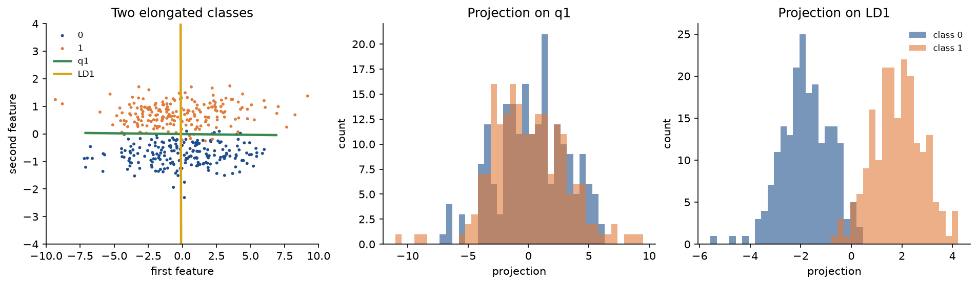
The direction of largest variance runs along both classes, so projecting onto it mixes them; the discriminant runs across the gap.

• Centring a new kernel with its own statistics. New points in kernel PCA must be centred with the training kernel's means. Treating the new kernel rows as a training set of their own shifts the projections of 50 fresh points on the circles by up to 0.0325, as examples/common_mistakes.py measures, and the error grows when the new points differ from the training set. Choose γ with care too: on the circles the first kernel component separates the rings perfectly for γ = 2 and γ = 5, but a nearest-centroid rule on it scores only 0.48 at γ = 0.5 and 0.63 at γ = 100, against 0.475 for linear PCA; examples/kernel_pca_and_lda.py sweeps the widths.

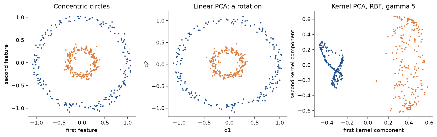
A linear method can only rotate and stretch the rings; in the kernel's feature space the radius becomes a direction, and the first kernel component splits the classes.

• LDA with many features and few rows. With 38 features of pure noise and 40 training rows in two classes, LDA separates the training rows perfectly in every one of 20 draws and scores 0.4975 on held-out rows on average. Shrink the within-class scatter, reduce the features first inside the pipeline, or regularize; and remember that LDA returns at most C − 1 directions. examples/kernel_pca_and_lda.py prints the averages.
• Over-reading a t-SNE map. Cluster sizes are equalized and gaps depend on the perplexity: in the blob experiment a width ratio of 5.25 becomes 1.20 at perplexity 30, and a gap ratio of 4.92 becomes 1.09, 2.87 or 9.11 at perplexities 5, 30 and 100. At low perplexity pure noise shows clumps. Compare several perplexities and seeds, and confirm clusters in the original space. t-SNE also cannot place new points, and scikit-learn's TSNE has no transform, so fitting it on all rows and then evaluating a classifier on the map is leakage. examples/tsne_maps.py prints the ratios, and the notebook's section on t-SNE draws the maps.

Further reading

• K. Pearson, "On lines and planes of closest fit to systems of points in space", Philosophical Magazine 2(11), 559-572, 1901. PCA as the closest subspace.
• H. Hotelling, "Analysis of a complex of statistical variables into principal components", Journal of Educational Psychology 24, 417-441 and 498-520, 1933. PCA as variance maximization.
• C. Eckart and G. Young, "The approximation of one matrix by another of lower rank", Psychometrika 1(3), 211-218, 1936.
• I. T. Jolliffe, Principal Component Analysis, second edition, Springer, 2002, and I. T. Jolliffe and J. Cadima, "Principal component analysis: a review and recent developments", Philosophical Transactions of the Royal Society A 374, 20150202, 2016.
• J. L. Horn, "A rationale and test for the number of factors in factor analysis", Psychometrika 30(2), 179-185, 1965. Parallel analysis.
• T. P. Minka, "Automatic choice of dimensionality for PCA", Advances in Neural Information Processing Systems 13, 2000.
• N. Halko, P.-G. Martinsson and J. A. Tropp, "Finding structure with randomness: probabilistic algorithms for constructing approximate matrix decompositions", SIAM Review 53(2), 217-288, 2011. Randomized SVD.
• A. Kessy, A. Lewin and K. Strimmer, "Optimal whitening and decorrelation", The American Statistician 72(4), 309-314, 2018. PCA, ZCA and other whitening transforms compared.
• B. Schölkopf, A. Smola and K.-R. Müller, "Nonlinear component analysis as a kernel eigenvalue problem", Neural Computation 10(5), 1299-1319, 1998. Kernel PCA.
• R. A. Fisher, "The use of multiple measurements in taxonomic problems", Annals of Eugenics 7(2), 179-188, 1936. The discriminant criterion.
• T. Hastie, R. Tibshirani and J. Friedman, The Elements of Statistical Learning, second edition, Springer, 2009, sections 4.3 (linear discriminant analysis) and 14.5 (principal components and curves).
• P. Baldi and K. Hornik, "Neural networks and principal component analysis: learning from examples without local minima", Neural Networks 2(1), 53-58, 1989. Linear autoencoders learn the PCA subspace.
• L. van der Maaten and G. Hinton, "Visualizing data using t-SNE", Journal of Machine Learning Research 9, 2579-2605, 2008.
• L. van der Maaten, "Accelerating t-SNE using tree-based algorithms", Journal of Machine Learning Research 15, 3221-3245, 2014.
• M. Wattenberg, F. Viégas and I. Johnson, "How to use t-SNE effectively", Distill, 2016. Interactive examples of the distortions described above.
• D. Kobak and P. Berens, "The art of using t-SNE for single-cell transcriptomics", Nature Communications 10, 5416, 2019, and A. C. Belkina et al., "Automated optimized parameters for t-distributed stochastic neighbor embedding improve visualization and analysis of large datasets", Nature Communications 10, 5415, 2019. Practical settings, including the learning rate used here.
• L. McInnes, J. Healy and J. Melville, "UMAP: uniform manifold approximation and projection for dimension reduction", arXiv:1802.03426, 2018.
• D. Kobak and G. C. Linderman, "Initialization is critical for preserving global data structure in both t-SNE and UMAP", Nature Biotechnology 39, 156-157, 2021.
• J. Venna and S. Kaski, "Neighborhood preservation in nonlinear projection methods: an experimental study", Artificial Neural Networks, ICANN 2001, 485-491. Trustworthiness.
• E. Alpaydin and C. Kaynak, "Optical Recognition of Handwritten Digits", UCI Machine Learning Repository, 1998, https://archive.ics.uci.edu/ml/datasets/Optical+Recognition+of+Handwritten+Digits.
• M. Forina et al., "Wine", UCI Machine Learning Repository, 1991, https://archive.ics.uci.edu/dataset/109/wine.