Naive Bayes¶

A spam filter has to decide, from the words of a message, whether it is spam. Bayes' rule turns the question around: how likely are these words if the message is spam, and how likely if it is not? Answering that for a whole message is hopeless, because almost every message is unique, so naive Bayes assumes that the words are independent once the class is known. The assumption is false for every real text, yet the classifier it produces trains in a single pass of counting, needs very little data, handles tens of thousands of features and often classifies remarkably well. This page derives the classifier from the Bayes-optimal decision rule, develops the Gaussian, Bernoulli, multinomial and complement variants, works a seven-message spam-or-ham example by hand with every count and probability shown, explains why smoothing and log-space arithmetic are not optional, and shows with a duplicated feature why the probabilities naive Bayes reports are overconfident even when its decisions are good. A complete spam filter, with a tokenizer and vocabulary built from scratch, then runs on an openly licensed corpus of text messages, chooses its smoothing by cross-validation, recalibrates its probabilities and explains its verdict on new messages. Afterwards you will be able to compute a naive Bayes posterior on paper, implement every variant in a few lines of NumPy, choose the variant and the smoothing for a problem, and know when its probabilities can be trusted. It builds on Probability and statistics.

To run the code in this topic, install the base group, and the ml group for the comparisons with scikit-learn.

Intuition¶

Think of every word of a message as a witness. Each witness says how much more often it turns up in spam than in ham, the ordinary messages, and the verdict weighs all the testimony together with the base rate of spam. In the language of odds:

Start with the prior odds of spam, the ratio of spam to ham in the training data.
Every word multiplies the odds by its likelihood ratio, its probability in spam divided by its probability in ham. "prize" might multiply them by 50, "lunch" divide them by 20.
The final odds give the posterior probability of spam.

Taking logarithms turns the multiplications into additions: the log odds of spam are the log prior odds plus one term of evidence per word. That one picture explains most of this page. Every word needs a finite, non-zero probability in every class, or a single word ends the trial; that is what smoothing guarantees. Products of hundreds of small probabilities vanish in floating point, sums of their logarithms do not. And since the witnesses are assumed to be independent, two witnesses who repeat each other are believed twice: the sign of the total, and so the decision, is often still right, but its size, and so the reported probability, is exaggerated.

The independence assumption is a statement about how the data are generated:

The generative story of naive Bayes: the prior picks a class y, spam or ham, and the class alone then draws each feature x1, x2 up to xd on its own, with no arrows between the features

First the prior picks a class, then each feature is drawn from its own distribution for that class, without looking at the other features. A model that describes how inputs are generated from classes is called generative, and classifying with it means running Bayes' rule backwards, from the features to the class. Logistic regression instead learns the posterior directly, and the two turn out to share the same form of decision boundary for discrete features.

How it works¶

Notation¶

The quantities on this page are:

The classes c run from 1 to K; a spam filter has K = 2, and with two classes they are called 0 and 1.
An example has the features x = (x1, ..., xd) and the class y. For text, the feature of token w is the number of times w occurs in the document.
The prior π of class c is the probability P(y = c); p(x | c) is the class-conditional probability or density of the features, and P(c | x) the posterior probability of class c.
V is the vocabulary of tokens and |V| its size.
N is the number of training examples and N(c) the number labelled c.
For text, n(c, w) is the total count of token w in the training documents of class c, n(c) the sum of these counts over all tokens, and N(c, w) the number of training documents of class c that contain w.
θ(c, w) is the probability of token w under class c, whose meaning depends on the variant, and α ≥ 0 is the strength of smoothing.
σ is the logistic sigmoid, 1 / (1 + e^(-z)), and Φ the standard normal distribution function.

The formula images write the class and the token as subscripts; the text writes them in parentheses, as in θ(c, w). Probability itself and Bayes' rule are treated in Probability and statistics.

Bayes' rule and the Bayes-optimal classifier¶

Bayes' rule writes the posterior in terms of quantities that can be estimated from labelled data:

The posterior of class c given x is the prior of c times the likelihood of x under c, divided by the evidence p of x, which is the sum over all classes k of prior times likelihood

The evidence p(x) is the same for every class. It does not affect which class has the largest posterior, but it is what makes the posteriors add up to one.

Why the largest posterior? Let h be any classifier and measure it by its probability of error, the expected 0-1 loss. Conditioning on the features, the error is the expected posterior mass of all the classes h does not choose:

The probability that h of x differs from y is the expectation over x of the sum over classes of the posterior of c times the indicator that h of x differs from c, which equals the expectation of one minus the posterior of the class h chooses

The expectation is smallest when the bracket is smallest for every x separately, that is when h(x) is the class with the largest posterior. The Bayes-optimal classifier, and its error, are therefore:

The Bayes-optimal classifier h star picks the class with the largest posterior, which is the class with the largest prior times likelihood; its error R star is the expectation of one minus the largest posterior

The error R*, the Bayes error, is the lowest error any classifier can achieve. It is zero only when the classes never overlap. Every practical classifier, naive Bayes included, can be judged by how close it gets to it.

Errors rarely cost the same. If calling a real message spam costs L(fp), a false positive, and letting spam through costs L(fn), a false negative, the expected cost of each decision and the rule that minimizes it are:

Predicting spam costs one minus the posterior of spam times the cost of a false positive, predicting ham costs the posterior of spam times the cost of a false negative, so spam is the cheaper prediction when its posterior exceeds the false-positive cost divided by the sum of both costs

If losing a real message is nine times as bad as receiving a spam, the threshold is 0.9. This rule only works with probabilities that mean what they say, which is exactly where naive Bayes is weakest, as the section on calibration below shows.

The naive assumption¶

Estimating p(x | c) directly is impossible for realistic inputs. With d binary features a full table of p(x | c) has 2^d - 1 free entries per class: for d = 30 that is 1,073,741,823, far more than any training set could fill. Naive Bayes assumes that the features are conditionally independent given the class:

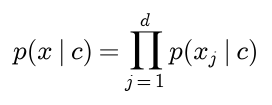
The likelihood of x under class c is the product over the d features of the likelihood of each feature under c

That leaves d one-dimensional distributions per class, 30 numbers in the example. Taking logarithms, the decision rule becomes a sum, the score of each class, and the posterior is the normalized exponential of the scores:

The score of class c is the log prior plus the sum over features of the log likelihood of each feature; the prediction is the class with the largest score, and the posterior of c is the exponential of its score divided by the sum of the exponentials of all scores

For two classes the log odds split into a prior term and one term of evidence per feature, the λ of feature j:

The log odds of class 1 against class 0 are the log of the prior ratio plus the sum over features of lambda j, where lambda j is the log of the ratio of the feature's likelihoods under class 1 and class 0

The variants below differ only in the one-dimensional model of each feature. The priors are always estimated by the class shares, N(c) / N, which is their maximum-likelihood estimate.

Gaussian naive Bayes¶

For continuous features each feature has a normal density with its own mean μ and variance σ² per class:

The log density of feature j under class c is minus one half the log of two pi sigma squared, minus the squared distance from the mean divided by twice the variance

The maximum-likelihood estimates are the class mean and the class variance with divisor N(c), not N(c) - 1:

The estimated mean is one over N c times the sum of the feature over the examples of class c, and the estimated variance is one over N c times the sum of squared deviations from that mean

For two classes, expanding the squares in the log odds and collecting powers of each feature gives a quadratic with coefficients a and b per feature and a constant c0:

The log odds are the sum over features of a j x j squared plus b j x j, plus c 0; a j is one half the difference of the inverse variances, b j the difference of mean over variance, and c 0 collects the log prior ratio, the log variance ratios and the squared means over variances

The decision boundary is the set where this expression is zero. Three consequences follow.

The boundary is a quadric, but an axis-aligned one: there are no cross terms between two features, because the model has no covariances. In two dimensions it is an ellipse, a hyperbola or a parabola whose axes are parallel to the coordinate axes.
In one dimension the boundary is the set of roots of a quadratic, so there can be two thresholds. The class with the larger variance wins far out on both sides, even on the side where the other class's mean lies. The worked example below has exactly this shape.
If every feature's variance is shared by the classes, then every a is zero and the log odds are linear, a weighted sum of the features plus a constant, with the weight of a feature equal to the difference of its two means divided by the shared variance. That is the functional form of logistic regression; the two differ in how they choose the weights.

A variance of zero, from a feature that is constant within a class, makes the density infinite. scikit-learn adds ε = 10⁻⁹ times the largest variance of any feature over all training data, the default var_smoothing, to every variance, and our implementation does the same so that the two agree. The Pitfalls section shows that this prevents a division by zero but not an absurd answer.

Bernoulli naive Bayes¶

For text, the simplest features record only whether each vocabulary token occurs, a 1 or a 0, and θ(c, w) is the probability that a document of class c contains w:

The likelihood of x under class c is the product over the whole vocabulary of theta to the power x w times one minus theta to the power one minus x w, and theta is estimated by the share of class c documents that contain w

The product runs over the whole vocabulary: an absent token contributes the factor 1 - θ(c, w), so not containing a word typical of ham is evidence for spam. The log odds are still linear in the features, with a constant that sums over every vocabulary token:

The log odds are the log prior ratio, plus the sum over the vocabulary of the log ratio of the absence probabilities, plus the sum over the vocabulary of x w times the log of the odds ratio of the token's presence

Repeated words count once.

Multinomial naive Bayes¶

The multinomial model treats a document of L tokens as L independent draws from the class's token distribution, one θ(c, w) per token, adding up to one over the vocabulary:

The likelihood of x under class c is a multinomial coefficient M of x times the product over the vocabulary of theta to the power of the count, where M of x is L factorial divided by the product of the count factorials; the score is the log prior plus the sum over tokens of count times log theta, plus a constant

The multinomial coefficient does not depend on the class and cancels in the posterior. The score is linear in the counts, a token that occurs twice counts twice, and absent tokens contribute nothing, unlike in the Bernoulli model. Equivalently, the score multiplies θ(c, w) once for every token position in the document, which is how the worked example computes it.

The maximum-likelihood estimate maximizes the log likelihood of the training counts subject to the constraint that the probabilities add up to one. With a Lagrange multiplier λ, three lines suffice:

The Lagrangian is the sum of n c w times log theta minus lambda times the sum of theta minus one; setting its derivative to zero gives theta equal to n c w over lambda; the constraint then forces lambda to equal n c, so the estimate is n c w divided by n c

The estimate n(c, w) / n(c) is the share of token w among all tokens of class c, as if the class's documents were concatenated into one long document.

Binary multinomial naive Bayes clips every count at one within each document, both in training and in scoring, and otherwise keeps the multinomial model. For short texts such as reviews or messages, whether a word occurs matters more than how often. It is not the Bernoulli model: absent tokens still contribute nothing, and θ is still one distribution over the vocabulary per class.

Smoothing and the zero-frequency problem¶

If token w never occurs in the training documents of class c, then its estimate θ(c, w) is 0, and every document containing w gets p(x | c) = 0, whatever its other tokens say. One unseen token vetoes the class, and when every class has such a token all scores are zero and the posterior is 0 / 0. With thousands of rare words this is not an edge case but the normal situation. Add-α smoothing adds a pseudo-count α to every count:

The smoothed multinomial estimate is n c w plus alpha over n c plus alpha times the vocabulary size; the smoothed Bernoulli estimate is N c w plus alpha over N c plus two alpha

α = 1 is Laplace smoothing and 0 < α < 1 is often called Lidstone smoothing. The estimate has a Bayesian reading. Put a symmetric Dirichlet prior with parameter α on the token distribution of a class and multiply it by the likelihood of the counts:

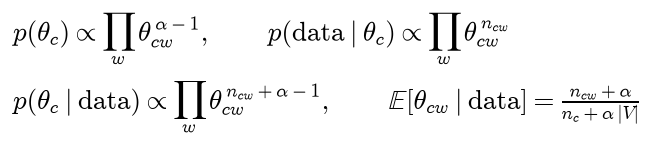
The Dirichlet prior is proportional to the product of theta to the power alpha minus one, and the likelihood to the product of theta to the power n c w; the posterior is proportional to the product of theta to the power n c w plus alpha minus one, and its mean is n c w plus alpha over n c plus alpha times the vocabulary size

The posterior is again a Dirichlet distribution, and its mean is exactly the add-α estimate. Laplace's choice α = 1 is the posterior mean under the uniform prior over all token distributions; the Bernoulli version is the same argument with a Beta(α, α) prior.

α moves the estimates between two extremes. As α approaches 0 they approach the raw frequencies, with their vetoes and their overconfidence. As α grows without bound every estimate approaches 1 / |V| in every class, every term of evidence approaches zero and the posterior falls back to the prior. The best α is a hyperparameter, chosen by cross-validation; α = 1 is a default, not a law. The same smoothing problem, with more refined answers, appears in N-gram language models.

Tokens that never occur in any training document are not in the vocabulary and are dropped from new documents. Scoring them with the smoothed estimate α / (n(c) + α |V|) instead looks harmless, since their count is zero in every class, but the denominators differ between classes, so each unknown token casts a vote for the class with fewer training tokens.

Log-space arithmetic¶

The smallest positive double-precision number is about 4.94 × 10⁻³²⁴, the smallest single-precision number about 1.40 × 10⁻⁴⁵. If the tokens of a message have probabilities around 10⁻³, a common size with a vocabulary of thousands of words, the product of their probabilities passes below the double-precision floor after about 324 / 3 = 108 tokens and becomes exactly zero, in every class at once. Sums of logarithms of the same numbers are a few hundred in size and lose nothing, so every implementation works with scores, never with products.

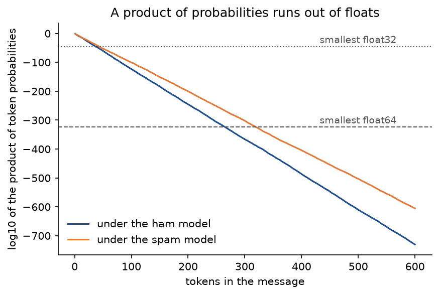
The log of the product of token probabilities against the number of tokens in a message drawn from the worked-example spam model: the ham and the spam line both fall steadily, crossing the single-precision floor after about forty tokens and the double-precision floor at about 265 and 320 tokens

The plot, from examples/log_space.py, follows a 600-token message drawn from the spam distribution of the worked-example model below. The product of token probabilities is exactly zero from token 265 for ham and token 320 for spam in double precision, and from tokens 37 and 44 in single precision; the posterior computed from the products is then 0 / 0, while the sums of logs give log odds of spam of 287.5 without trouble. With a realistic vocabulary each factor is far smaller and the product underflows sooner.

Turning scores back into posteriors needs the logarithm of a sum of exponentials, and computing it naively reintroduces the underflow, since every exponential may be zero. The log-sum-exp identity avoids it. Writing s for the scores and m for the largest of them:

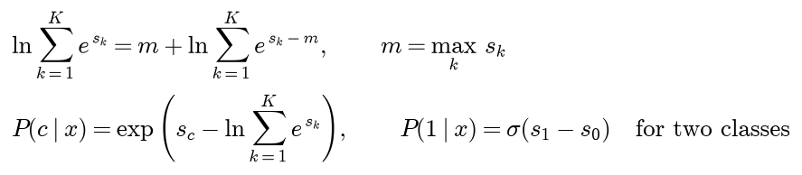
The log of the sum of e to the s k equals m plus the log of the sum of e to the s k minus m, with m the largest score; the posterior of c is the exponential of s c minus that log-sum-exp, and for two classes the posterior of class 1 is the sigmoid of s 1 minus s 0

The identity holds because the sum of the exponentials is e^m times the sum of the shifted exponentials. Every shifted term is at most one and the largest is exactly one, so the sum lies between 1 and K: nothing overflows, nothing underflows to zero, and the logarithm is safe. For the Bernoulli model, log(1 - θ) is computed with log1p so that tiny θ lose no precision.

Why naive Bayes ranks well but calibrates poorly¶

Naive Bayes adds one term of evidence per feature. When features carry the same information, that information is added more than once.

Duplication first. Suppose feature j is the only informative feature, the priors are equal, and the feature is copied so that it appears k times. Each copy contributes the same λ, so naive Bayes reports log odds k λ while the true log odds are λ. Multiplying by k > 0 keeps the order, so the order of examples, and with it every ranking measure such as the ROC AUC, is unchanged; the sign is unchanged, so every decision is unchanged. Only the probabilities move. If p = σ(z) is the true posterior, the reported posterior is:

Sigma of k z equals one over one plus the k-th power of one minus p over p, which equals p to the k over p to the k plus one minus p to the k, where p is sigma of z

A true 0.8 becomes 0.512 / (0.512 + 0.008) = 0.9846 with three copies: the model sounds almost certain about a case it should get wrong one time in five.

Correlation is a softer version of the same thing. Let two features be equally informative and correlated inside each class: normally distributed with means (0, 0) for class 0 and (δ, δ) for class 1, unit variances and correlation ρ, so the covariance matrix Σ has ones on the diagonal and ρ off it. With a covariance shared by the classes the true log odds are linear, and because the vector (1, 1) is an eigenvector of Σ they simplify:

The true log odds are the transposed mean difference times the inverse covariance times x, minus one half the difference of the two quadratic forms of the means; since Sigma times the vector of ones is one plus rho times that vector, the log odds equal delta times x 1 plus x 2, minus delta squared, all over one plus rho

Naive Bayes uses only the marginal variances, which are 1, and arrives at δ(x1 + x2) - δ²: exactly 1 + ρ times the truth. Its decisions are Bayes-optimal and its ranking is perfect, but it counts the evidence 1 + ρ times, and ρ = 1 is exact duplication with factor 2.

When the redundancy is spread unevenly, the overcounting also changes the relative weight of the features, and then ranking and accuracy suffer too. For two Gaussian classes with equal priors and a shared covariance this can be computed in closed form. Any linear rule that compares a weighted sum of the features, with weights w, against a threshold midway between the two class means has the error:

The error of the linear rule with weights w is Phi of minus w transposed times the mean difference, divided by twice the square root of w transposed Sigma w

The Bayes-optimal weights, and the weights naive Bayes converges to with unlimited data because it sees only the diagonal D of Σ, are:

The Bayes-optimal weights are the inverse covariance times the mean difference, which gives the Bayes error Phi of minus Delta over two, with Delta squared the Mahalanobis distance between the means; naive Bayes uses the inverse of the diagonal of Sigma instead

For a mean difference of (1.5, 0.5) and ρ = 0.6 the Bayes error is 0.2146 and the naive rule's error 0.2489; for (1.5, 1.0) and independent features both are 0.1837; for (1, 1) and ρ = 0.5 both are 0.2819, as the symmetric argument above predicts. The general lesson, made precise by Domingos and Pazzani, is that a classifier only needs the right sign of the log odds to classify and the right order to rank, and naive Bayes often gets both while badly misjudging the size.

Recalibration fixes the size without touching the order. Platt scaling fits a sigmoid with slope a and intercept b to the scores of held-out examples by maximum likelihood:

Platt scaling: the recalibrated probability of class 1 is the sigmoid of a times the score plus b

With k duplicated copies the fitted slope is close to 1 / k, and in general 1 / a estimates how many times the evidence is being counted.

examples/independence_assumption.py measures all of this with Gaussian naive Bayes and pooled variances, the right model for the data before any copying, trained on 500 points per class, with 2,000 further points per class for the Platt fit and 10,000 for testing. In the first experiment the only feature is copied k times:

One copy: accuracy 0.6906, ROC AUC 0.7620, log loss 0.5798, calibration error 0.0119, Platt slope 1.0899.
Two copies: log loss 0.6368, calibration error 0.1040, Platt slope 0.5449.
Three copies: log loss 0.7615, calibration error 0.1597, Platt slope 0.3633.
Five copies: log loss 1.0834, calibration error 0.2142, Platt slope 0.2180.
Ten copies: log loss 1.9981, calibration error 0.2604, Platt slope 0.1090.

The accuracy and the ROC AUC do not change in any digit, the Platt slope falls exactly as 1 / k times its value for one copy, and the log loss more than triples. In the second experiment there are two equally informative features and the first is copied, so the copies also tilt the weights: the ROC AUC falls from 0.8417 with one copy through 0.8227, 0.8077 and 0.7913 to 0.7762 with ten, while the log loss grows four and a half times, from 0.4923 to 2.2332.

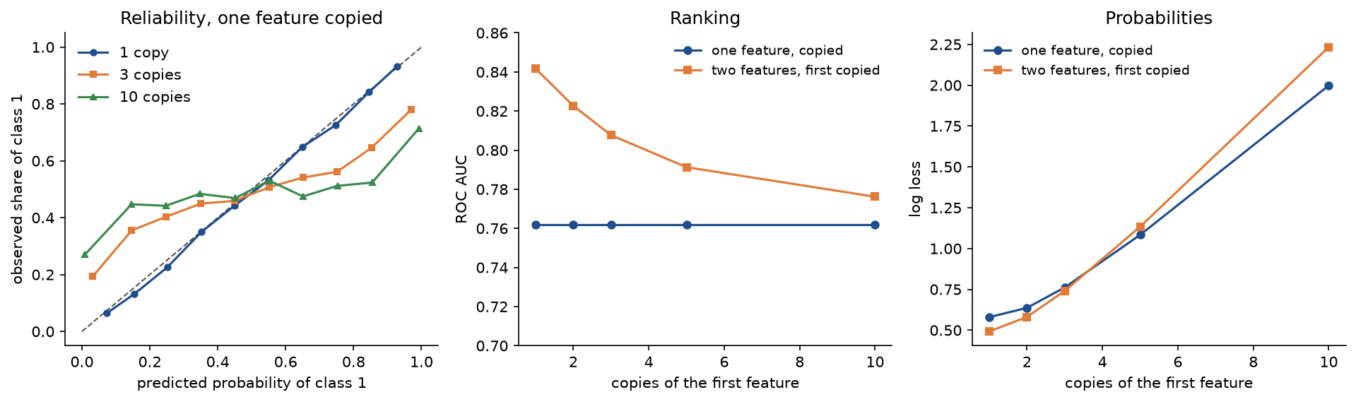
Three panels for copies of a feature: reliability curves for one, three and ten copies of a single feature, which bend away from the diagonal as copies are added; the ROC AUC against the number of copies, flat for one copied feature and falling for two features; and the log loss against the number of copies, rising steeply in both experiments

The reliability curves flatten as copies are added: predictions near 0 and 1 become far more common than the outcomes justify. The middle panel shows that only uneven duplication touches the ranking, and the right panel that the probabilities suffer in both cases.

For two equally informative features with within-class correlation ρ, 5,000 training and 20,000 test points per class, the naive error stays within sampling noise of the Bayes error while the Platt slope follows 1 / (1 + ρ):

ρ = 0: Bayes error 0.2398, naive Bayes error 0.2429, log loss 0.4959 for the true posterior and 0.4960 for naive Bayes, Platt slope 0.9859 against 1.
ρ = 0.3: errors 0.2676 and 0.2706, log losses 0.5348 and 0.5429, Platt slope 0.7627 against 0.7692.
ρ = 0.6: errors 0.2881 and 0.2917, log losses 0.5608 and 0.5870, Platt slope 0.6229 against 0.6250.
ρ = 0.9: errors 0.3040 and 0.3070, log losses 0.5792 and 0.6297, Platt slope 0.5262 against 0.5263.

The Bayes error itself is reached when the assumption holds, and learning curves show how fast:

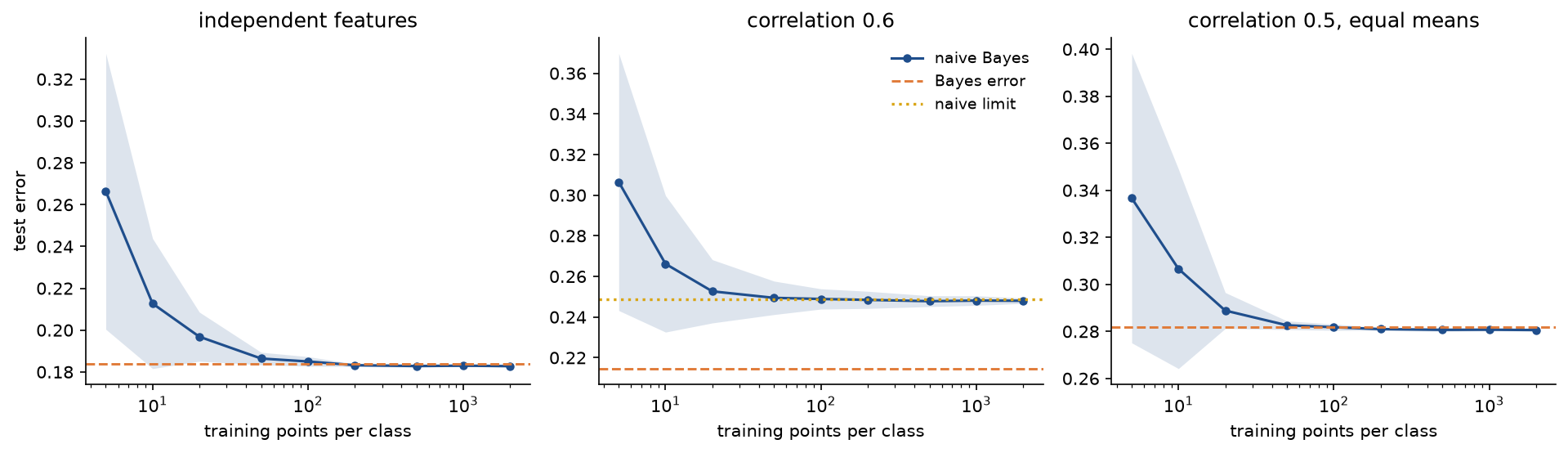
Test error of Gaussian naive Bayes against the number of training points per class in three settings, with a band of one standard deviation: with independent features it falls to the Bayes error, with correlation 0.6 it levels off at the dotted naive limit well above the dashed Bayes error, and for the symmetric correlated pair it reaches the Bayes error

Each curve averages 40 training sets per size, tested on 20,000 fresh points per class. With 2,000 training points per class, the test error is 0.1828 against a Bayes error of 0.1837 for independent features, levels off at 0.2480 against 0.2146 for features with correlation 0.6 whose correlation changes the best direction (the limit of the naive rule is 0.2489), and reaches 0.2806 against 0.2819 for the symmetric correlated pair, where correlation leaves the best direction alone. Test errors slightly below the Bayes error are sampling noise of the 40,000 test points.

Complement naive Bayes¶

With many classes of very different sizes, the multinomial estimates of a small class rest on few tokens and the model drifts towards large classes. Complement naive Bayes estimates, for each class, the token distribution of all the other classes, which always has plenty of data, and prefers the class whose complement fits the document worst:

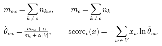
The complement counts m c w and m c sum the counts of all classes other than c; the complement estimate is m c w plus alpha over m c plus alpha times the vocabulary size, and the score of c is minus the sum over tokens of the count times the log complement estimate

The prior is not used. An optional normalization divides each class's weights, the logarithms of its complement estimates, by their sum, which stops classes with long documents from dominating. With two classes the complement of class 0 is class 1, so the complement estimate of class 0 is the ordinary estimate of class 1 and the score difference is:

The score of class 1 minus the score of class 0 is the sum over tokens of the count times the difference of the log estimates of class 1 and class 0

This is the multinomial log odds without the prior term. For a binary problem complement naive Bayes is therefore multinomial naive Bayes with uniform priors; its benefit appears with many unbalanced classes.

Worked example¶

Spam or ham by hand¶

Seven training messages, already lowercased and split into tokens, and one new message, "call now to claim free cash":

Spam: "win cash now", "free cash prize now now" and "claim free prize".
Ham: "call me now", "lunch at noon", "free for lunch call me" and "call me at noon".

Every value below is computed in double precision and rounded to four decimals for display.

Priors and counts. There are four ham and three spam messages, so the prior of ham is 4/7 = 0.5714 and the prior of spam 3/7 = 0.4286. The vocabulary has 12 tokens. In ham the counts are at 2, call 3, for 1, free 1, lunch 2, me 3, noon 2 and now 1, 15 tokens in all; in spam they are cash 2, claim 1, free 2, now 3, prize 2 and win 1, 11 tokens in all. The new message has the tokens call, now, to, claim, free and cash. "to" is not in the vocabulary and is dropped, which leaves five tokens.

Without smoothing. The raw estimates are the counts divided by the class totals. For spam, "call" has count 0, so its estimate is 0/11 = 0 and the spam score is zero. For ham, "claim" and "cash" have count 0, so the ham score is zero as well. Both products are exactly 0 and the posterior is 0 / 0: the classifier cannot decide at all, although four of the five tokens point clearly to spam.

With Laplace smoothing, α = 1. The denominators are 11 + 12 = 23 for spam and 15 + 12 = 27 for ham. For each token, the spam estimate, the ham estimate and the evidence, the log of their ratio:

call: 1/23 = 0.0435 and 4/27 = 0.1481, evidence -1.2260.
now: 4/23 = 0.1739 and 2/27 = 0.0741, evidence 0.8535.
claim: 2/23 = 0.0870 and 1/27 = 0.0370, evidence 0.8535.
free: 3/23 = 0.1304 and 2/27 = 0.0741, evidence 0.5658.
cash: 3/23 = 0.1304 and 1/27 = 0.0370, evidence 1.2590.

"now" and "claim" carry the same evidence because both ratios equal 54/23. Prior times likelihood for each class, and the posterior after dividing by their sum, the evidence p(x):

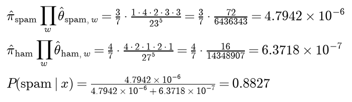
For spam, three sevenths times 1 times 4 times 2 times 3 times 3 over 23 to the fifth, which is three sevenths times 72 over 6436343, equals 4.7942 times ten to the minus 6; for ham, four sevenths times 16 over 27 to the fifth, 14348907, equals 6.3718 times ten to the minus 7; the posterior of spam is the first divided by the sum of both, 0.8827

So P(spam | x) = 0.8827 and P(ham | x) = 0.1173.

In log space. The log prior of spam is -0.8473 and the log factors, in the order call, now, claim, free and cash, are -3.1355, -1.7492, -2.4423, -2.0369 and -2.0369, so the spam score is -12.2481. For ham the log prior is -0.5596 and the log factors are -1.9095, -2.6027, -3.2958, -2.6027 and -3.2958, so the ham score is -14.2662; the sum of the rounded terms is -14.2661, one unit higher in the last digit than the full-precision value. Log-sum-exp with m = -12.2481 gives -12.2481 + ln(1 + e^(-2.0181)) = -12.1233, so the log posteriors are -0.1248 for spam and -2.1429 for ham, which exponentiate to 0.8827 and 0.1173. Neither score is ever turned back into a tiny probability.

As a sum of evidence. The log prior odds of spam are ln(3/4) = -0.2877, and the five terms of evidence add to the log odds:

The worked message as a sum of evidence: the prior odds of 3 to 4 with log -0.2877 and the token call with -1.2260 point to ham, now and claim with +0.8535 each, free with +0.5658 and cash with +1.2590 point to spam, the unknown token to is dropped, the sum 2.0181 is the log odds of spam, and its sigmoid 0.8827 the posterior

-0.2877 - 1.2260 + 0.8535 + 0.8535 + 0.5658 + 1.2590 = 2.0181, and σ(2.0181) = 0.8827. "call" is the only witness for ham, and the prior leans slightly towards ham; the other four tokens outweigh both.

Binary multinomial. Clipping counts within each message changes only the second spam message, whose "now now" now counts once. The spam count of "now" drops to 2 and the spam total to 10, so the spam denominators become 10 + 12 = 22: call 1/22 = 0.0455, now 3/22 = 0.1364, claim 2/22 = 0.0909, free 3/22 = 0.1364 and cash 3/22 = 0.1364. The spam score becomes -12.3135, the ham score stays -14.2662, and P(spam | x) = 0.8757.

Bernoulli. Now each vocabulary token contributes, present or absent. The document counts equal the token counts above except for "now" in spam, which occurs in two of the three spam messages. The estimates are (N(c, w) + 1) / (N(c) + 2), with denominators 5 for spam and 6 for ham. The factor is the estimate for the five tokens present in the message and one minus the estimate for the seven absent ones; for each token, the spam factor and the ham factor:

at, absent: 1 - 1/5 = 0.8000 and 1 - 3/6 = 0.5000.
call, present: 1/5 = 0.2000 and 4/6 = 0.6667.
cash, present: 3/5 = 0.6000 and 1/6 = 0.1667.
claim, present: 2/5 = 0.4000 and 1/6 = 0.1667.
for, absent: 0.8000 and 1 - 2/6 = 0.6667.
free, present: 3/5 = 0.6000 and 2/6 = 0.3333.
lunch, absent: 0.8000 and 0.5000.
me, absent: 0.8000 and 1 - 4/6 = 0.3333.
noon, absent: 0.8000 and 0.5000.
now, present: 3/5 = 0.6000 and 2/6 = 0.3333.
prize, absent: 1 - 3/5 = 0.4000 and 1 - 1/6 = 0.8333.
win, absent: 1 - 2/5 = 0.6000 and 0.8333.

The logs of the twelve factors sum to -6.6010 for spam and -10.1344 for ham; adding the log priors gives scores -7.4483 and -10.6940, products 5.8241 × 10⁻⁴ and 2.2681 × 10⁻⁵, and P(spam | x) = 0.9625. The Bernoulli model is more confident than the multinomial one mostly because of absent tokens: three of the four ham messages contain "me", so its absence multiplies the odds of spam by 0.8 / 0.3333 = 2.4.

How much smoothing. The multinomial posterior of spam is 0.9993 for α = 0.01, 0.9920 for 0.1, 0.9473 for 0.5, 0.8827 for 1, 0.7746 for 2, 0.6170 for 5 and 0.4399 for 100. Small α makes the near-zero estimates for unseen tokens extreme and the posterior almost certain; large α flattens every estimate towards 1/12 and the posterior approaches the prior of spam, 0.4286.

A Gaussian boundary by hand¶

One feature, two classes with equal priors: class 0 has the points 1, 2 and 3 and class 1 the points 4, 6 and 8. The estimates, and the coefficients of the log odds from How it works:

The mean of class 0 is 2 and its variance 1 plus 0 plus 1 over 3, 0.6667; the mean of class 1 is 6 and its variance 4 plus 0 plus 4 over 3, 2.6667; a is one half of 1.5 minus 0.375, 0.5625; b is 6 over eight thirds minus 2 over two thirds, 2.25 minus 3, minus 0.75; c 0 is 0 minus one half log 4 minus one half of 13.5 minus 6, minus 4.4431

So the log odds of class 1 are 0.5625 x² - 0.75 x - 4.4431. Setting them to zero:

x equals 0.75 plus or minus the square root of 0.5625 plus 4 times 0.5625 times 4.4431, over 2 times 0.5625, which is 0.75 plus or minus 3.2496 over 1.125, so x is 3.5552 or minus 2.2218

The second root is -2.2219 from the rounded square root and -2.2218 at full precision.

Class 1 wins for x > 3.5552, as expected, and also for x < -2.2218, far to the left of both classes, because there the narrow density of class 0 falls off faster than the wide density of class 1. At x = 3.2 the log densities are -0.7162 - 1.08 = -1.7962 for class 0 and -1.4094 - 1.47 = -2.8794 for class 1. The log odds, 0.5625 × 3.2² - 0.75 × 3.2 - 4.4431 = -1.0831, give P(1 | x) = σ(-1.0831) = 0.2529; the difference of the two rounded log densities is -1.0832. At x = -3 the log odds are 0.5625 × 9 + 2.25 - 4.4431 = 2.8694 and P(1 | x) = 0.9463, at x = 0 only 0.0116. With a pooled variance, (0.6667 + 2.6667) / 2 = 1.6667 for both classes, the quadratic term vanishes and the single threshold is the midpoint 4. scikit-learn's var_smoothing adds 10⁻⁹ times the largest feature variance, here 5.67 × 10⁻⁹, to both variances, which changes none of the displayed digits.

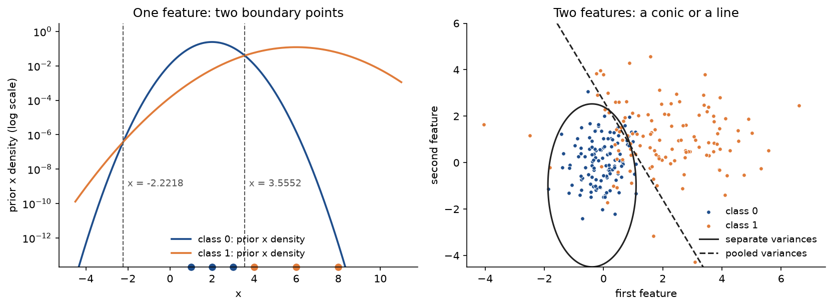
Left: prior times density of both classes of the one-feature example on a logarithmic axis, with the training points along the bottom and dashed lines at the two boundary points minus 2.2218 and 3.5552. Right: two classes in two dimensions with the boundary of Gaussian naive Bayes, an ellipse around the narrow class for separate variances and a straight dashed line for pooled variances

On the logarithmic axis the second crossing is visible far out on the left, where both densities are tiny. The right panel, with 120 points per class, shows the axis-aligned ellipse that separate variances produce and the straight line of pooled variances; the two reach training accuracies of 0.8833 and 0.8667.

Every number in this section is asserted by tests/test_trace.py and tests/test_gaussian.py, and printed by examples/worked_example.py and examples/gaussian_boundary.py.

The code¶

The package naive_bayes is plain NumPy, split into one module per idea. SciPy is imported only inside SparseCounts.to_scipy, scikit-learn only inside the functions of comparisons.py, and Pillow only when a figure has to be shrunk.

arrays.py holds the array types, encode_labels, which sorts the classes as scikit-learn does, and class_column.
log_space.py holds log_sum_exp, an overflow-free sigmoid, log_ratio, which turns a zero count into minus infinity quietly, and the helpers that measure underflow.
sparse.py holds SparseCounts, a compressed sparse row matrix, and the two operations every discrete model is built from: class_totals, the counts per class, and linear_scores, features times a weight matrix touching only the non-zero entries.
text.py holds tokenize, build_vocabulary and vectorize.
model.py holds NaiveBayesModel, the base class that turns scores into predict_log_proba, predict_proba, predict and log_odds, and log_priors.
discrete.py holds MultinomialNaiveBayes (with binary=True for the binary variant), BernoulliNaiveBayes and ComplementNaiveBayes (with normalize), each a frozen dataclass with a fit class method.
gaussian.py holds GaussianNaiveBayes with var_smoothing, pooled_variance and boundary_quadratic, and boundary_points_1d.
trace.py holds the worked examples and trace_text_example, which keeps every count, factor and score of the text example, with format_text_trace to print them.
metrics.py holds accuracy, precision, recall, F1, confusion counts, the ROC AUC through average ranks, log loss, the Brier score and evaluate_binary.
calibration.py holds reliability tables, the expected calibration error, confident_errors, odds_power and fit_platt_scaling, Newton's method on Platt's smoothed targets.
bayes_error.py holds the closed-form errors of linear rules, the Bayes error and the naive rule for two Gaussian classes.
datasets.py generates the synthetic data from seeds.
experiments.py runs the controlled experiments with copied and correlated features and the learning curves.
underflow.py scores a long message with products and with logs.
sms.py downloads, verifies, parses and deduplicates the SMS corpus, and corpus.py turns it into a stratified split counted over a training vocabulary.
validation.py holds stratified splits and folds, vectorize_folds, which rebuilds the vocabulary inside every fold, sweep_alpha, out_of_fold_log_odds and VARIANTS, the four discrete variants by name.
explain.py holds top_tokens and explain_message, which splits one message's log odds into the prior and the evidence of each token.
pitfalls.py holds the deliberate mistakes of the Pitfalls section.
comparisons.py fits the scikit-learn counterparts and measures the agreement.
plotting.py and calibration_plots.py draw every figure in the handbook's four colours and save it reproducibly.

All three discrete variants are linear in the features, so they share one scoring routine. Training the multinomial model is counting plus two lines of smoothing:

counts = class_totals(features, class_index, classes.size)
smoothed = counts + alpha
feature_log_prob = log_ratio(smoothed, smoothed.sum(axis=1, keepdims=True))

and scoring is linear_scores(features, self.feature_log_prob) + self.class_log_prior. For sparse input linear_scores multiplies only the non-zero counts, so an absent token costs nothing, and a log probability of minus infinity for a token the document does not contain is never multiplied by its zero count, which would give nan. Posteriors go through log_sum_exp, which returns minus infinity rather than nan when every score is minus infinity.

The examples and the project import the package, so install the repository first as described in the main README. The examples each demonstrate one idea and run in a few seconds at most from the repository root:

examples/worked_example.py prints every value of the spam-or-ham example in the order above: counts, factors and posteriors with and without smoothing, the log-space computation, the sum of evidence, the binary multinomial and Bernoulli variants, and the posterior for seven values of α.
examples/gaussian_boundary.py reproduces the Gaussian worked example and saves the boundary figure.
examples/log_space.py measures where products of probabilities underflow and saves the underflow figure.
examples/independence_assumption.py computes the closed-form errors, the learning curves and the experiments with copied and correlated features, and saves their two figures.
examples/common_mistakes.py demonstrates the pitfalls below; its last part downloads the SMS corpus on first use.
examples/compare_with_sklearn.py checks every variant against scikit-learn on the worked examples, on random counts and on the SMS corpus, and compares three tokenizers.

python machine-learning/naive-bayes/examples/worked_example.py
python machine-learning/naive-bayes/examples/gaussian_boundary.py
python machine-learning/naive-bayes/examples/log_space.py
python machine-learning/naive-bayes/examples/independence_assumption.py
python machine-learning/naive-bayes/examples/common_mistakes.py
python machine-learning/naive-bayes/examples/compare_with_sklearn.py

The sample project: an SMS spam filter¶

project/spam_filter.py builds a complete spam filter on the SMS Spam Collection and then classifies new messages given on the command line, or four example messages written for it when none are given:

Nothing the test messages contain influences the model: the vocabulary, α and the calibration are all decided on the training messages. The run goes through these steps.

The corpus has 5,574 English text messages, 747 spam and 4,827 ham. Some messages occur several times, and a split of the raw corpus would put 133 of its 1,114 test messages next to an identical copy in the training set, where naive Bayes has already counted every one of their tokens. So the corpus is deduplicated first: 5,171 distinct messages, 653 spam and 4,518 ham.
A stratified split keeps 4,136 messages (522 spam) for training and 1,035 (131 spam) for testing; always predicting ham would score 0.8734 accuracy.
The tokenizer lowercases and keeps words with internal apostrophes, digit runs and the symbols £ $ € ! ?, and replaces every digit run of five or more characters by the single token <number>, because spam is full of phone numbers and short codes that are individually rare but collectively a strong signal. The vocabulary, built from the training messages only, has 7,159 tokens. The document-term matrix has 76,659 non-zero entries, 0.21 % of all cells, and stores in 1.3 MB instead of the 296 MB of a dense matrix.
Five stratified folds of the training messages, each with its own vocabulary, choose α for each of the four discrete variants from nine values between 0.001 and 10, by the lowest mean validation log loss: 0.316 for the multinomial, binary multinomial and complement variants and 0.1 for Bernoulli.
Every variant is evaluated once on the test messages, with α = 1 and with the chosen α.
The chosen filter, multinomial by default, is recalibrated with Platt scaling on out-of-fold log odds of the training messages, and its calibration is reported before and after.
Each new message is classified, with its log odds, the error the filter claims before and after recalibration, the tokens with the strongest evidence each way and the tokens it does not know.

python machine-learning/naive-bayes/project/spam_filter.py
python machine-learning/naive-bayes/project/spam_filter.py "URGENT! Your mobile won a prize, call 09012345678" "see you at the station"
python machine-learning/naive-bayes/project/spam_filter.py --variant "binary multinomial" --keep-numbers

Options such as --seed, --test-fraction, --folds, --variant, --min-document-frequency and --keep-numbers change the setup, and --figures sends the two PNGs to another folder so a custom run does not overwrite the ones shown here. The default run takes about two seconds once the corpus is downloaded. Test results with spam as the positive class, first with α = 1 and then with the chosen α, as accuracy, precision, recall, F1, ROC AUC and log loss:

Multinomial, α = 1: 0.9884, 0.9685, 0.9389, 0.9535, 0.9760 and 0.1102.
Binary multinomial, α = 1: 0.9884, 0.9685, 0.9389, 0.9535, 0.9780 and 0.0972.
Bernoulli, α = 1: 0.9807, 1.0000, 0.8473, 0.9174, 0.9890 and 0.2029.
Complement, α = 1: 0.9845, 0.9259, 0.9542, 0.9398, 0.9760 and 0.1211.
Multinomial, α = 0.316: 0.9884, 0.9612, 0.9466, 0.9538, 0.9782 and 0.1159.
Binary multinomial, α = 0.316: 0.9874, 0.9609, 0.9389, 0.9498, 0.9793 and 0.1066.
Bernoulli, α = 0.1: 0.9894, 0.9918, 0.9237, 0.9565, 0.9864 and 0.1237.
Complement, α = 0.316: 0.9845, 0.9197, 0.9618, 0.9403, 0.9782 and 0.1282.

The tuned multinomial filter misses 7 of the 131 spam messages and flags 5 of the 904 ham messages. The differences between the variants are a few messages each, and one spam message is worth 0.0076 of recall, so these numbers support only coarse conclusions. Complement naive Bayes trades precision for recall because, with two classes, it is the multinomial model without the prior that favours ham.

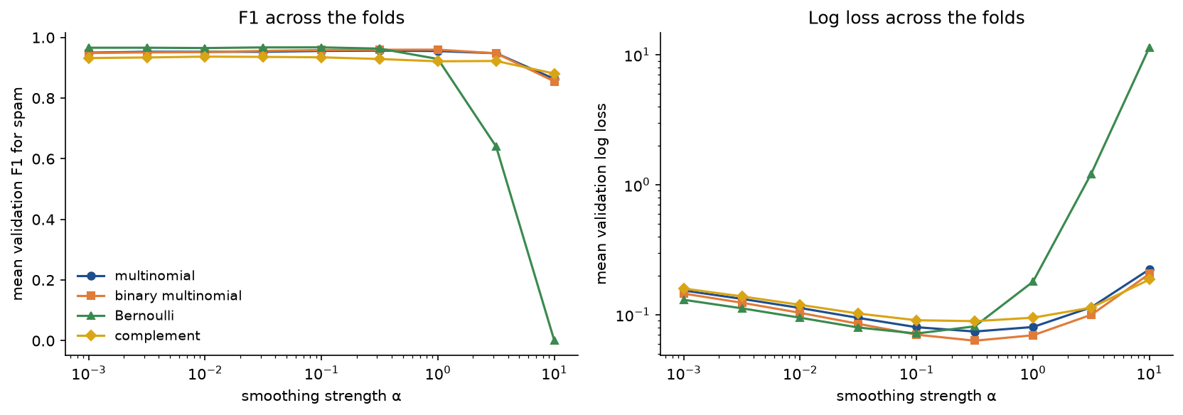
Mean validation F1 and mean validation log loss over five folds against the smoothing strength for the four discrete variants: three variants stay flat over most of the range, while Bernoulli collapses to an F1 of zero and a log loss above ten at alpha 10

The sweep shows why α has to be tuned per variant. Bernoulli naive Bayes is by far the most sensitive: its constant term sums log(1 - θ) over the whole vocabulary of several thousand tokens, and α shifts every one of them. Its mean validation F1 is 0.9674 at α = 0.1, 0.9290 at α = 1, and 0 at α = 10, where it labels no message as spam at all, while binary multinomial still reaches 0.8551 there.

The tokens with the largest evidence for spam are <number> (+8.62), 150, claim, prize, 16, won, tone, guaranteed, ppm, cs, awarded and 500; mapping every long digit run to one token turns hundreds of rare phone numbers and short codes into the strongest single signal. The strongest evidence for ham comes from gt (-5.31), lt, he, lor, ü, da, i'll, she, too, later, way and ask. "gt" and "lt" are remains of HTML-escaped placeholders such as <#>, which appear in 222 of the 4,518 distinct ham messages and in no spam: an artefact of how the ham messages were collected, which a model trained on this corpus learns as eagerly as real language. It is the kind of shortcut described in Data leakage and pitfalls.

The tuned multinomial filter is very sure of itself. 828 of the 1,035 test messages receive a claimed error below 10⁻⁴, a posterior above 0.9999 for the predicted class, and 5 of them are wrong, an error rate of 0.60 %; 353 messages have a claimed error below 10⁻¹⁰, and 2 of those are wrong. Platt scaling fitted on out-of-fold log odds of the training messages gives slope 0.2930 and intercept -1.6920: the filter counts its evidence about 1 / 0.2930 = 3.41 times, the text version of the duplicated feature. After recalibration the test log loss drops from 0.1159 to 0.0575, while the ROC AUC stays at 0.9782 because the transformation keeps the order. The Brier score, which charges a confident mistake at most 1, barely moves, from 0.0096 to 0.0098.

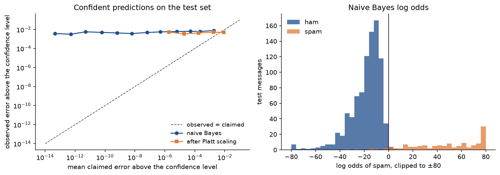
Left: the error rate observed among confident test predictions against the mean error the filter claims for them, on logarithmic axes, far above the diagonal for naive Bayes and close to it after Platt scaling. Right: histograms of the log odds of spam for ham and spam test messages, spread from minus 80 to plus 80

Before recalibration the filter claims errors below 10⁻¹³ for groups of messages whose observed error stays near half a percent; after Platt scaling the claims sit close to the observations. The histogram shows why: log odds of minus 20 to minus 40 are routine for ham, numbers that would mean near certainty if the evidence were not counted several times.

For the four default messages the verdicts read, for example, "spam, log odds of spam +42.68; claimed error 2.9e-19 raw, 2.0e-05 recalibrated" for a prize offer with a premium-rate number, with <number> (+8.62), claim (+6.73) and prize (+6.49) as the strongest witnesses, and "ham, log odds of spam -20.31; claimed error 1.5e-09 raw, 4.8e-04 recalibrated" for a lunch arrangement, where lunch (-3.49), bring (-2.97) and i (-2.69) speak for ham. The project prints counts, scores and individual tokens from the corpus, never whole corpus messages.

The notebook naive_bayes.ipynb is a guided tour in the order of this page: the worked example in all its variants, the Gaussian boundary, log space and underflow, the Bayes error and the overconfidence experiments, each pitfall, the spam filter step by step and the comparison with scikit-learn. The tests in tests check the worked examples value by value, the mathematical properties above and the agreement with scikit-learn, and run in a few seconds:

python -m pytest machine-learning/naive-bayes

Data: the synthetic Gaussian sets are generated from fixed seeds. The SMS Spam Collection v.1 by T. A. Almeida, J. M. Gómez Hidalgo and A. Yamakami is distributed by the UCI Machine Learning Repository under the Creative Commons Attribution 4.0 International licence (CC BY 4.0). load_sms_collection downloads the 203 KB archive from https://archive.ics.uci.edu/static/public/228/sms+spam+collection.zip on first use into .data/naive-bayes/ at the repository root, which is not committed, and verifies its pinned SHA-256 digest before use.

In practice¶

scikit-learn implements every variant here, and the correspondence is direct:

MultinomialNaiveBayes is MultinomialNB(alpha, fit_prior), which also accepts tf-idf weights.
MultinomialNaiveBayes(binary=True) is MultinomialNB on counts clipped at 1.
BernoulliNaiveBayes is BernoulliNB(alpha, binarize=0.0), which binarizes its input at the threshold.
ComplementNaiveBayes is ComplementNB(alpha, norm).
GaussianNaiveBayes is GaussianNB(var_smoothing), which has no pooled-variance option.

scikit-learn also offers CategoricalNB for features with a few unordered values, the Bernoulli model with more than two outcomes per feature. CountVectorizer with our tokenizer, lowercase=False and token_pattern=None, which count_vectorizer returns, builds exactly our vocabulary and document-term matrix, entry for entry. A filter in scikit-learn is then a few lines:

from sklearn.naive_bayes import MultinomialNB

from naive_bayes import count_vectorizer, prepare_sms_split

split = prepare_sms_split()
vectorizer = count_vectorizer()
train = vectorizer.fit_transform([split.messages[i] for i in split.train_index])
model = MultinomialNB(alpha=1.0).fit(train, split.train_labels)
test = vectorizer.transform([split.messages[i] for i in split.test_index])
print((model.predict(test) == split.test_labels).mean())

It prints the test accuracy 0.9884 of our multinomial model with α = 1. On the SMS test messages with α = 1, examples/compare_with_sklearn.py finds the largest difference between our log posteriors and scikit-learn's to be 1.4 × 10⁻¹⁴ for MultinomialNB and for the binary variant, 3.1 × 10⁻¹³ for BernoulliNB and 1.4 × 10⁻¹³ for ComplementNB, with every prediction identical, and 3.6 × 10⁻¹⁵ for GaussianNB on the two-dimensional data of the boundary figure. The tests check the same agreement on dense and sparse data with two and three classes, both settings of fit_prior and norm, and several values of α. The tokenizer matters as much as the variant. With MultinomialNB and α = 1, as vocabulary size, accuracy, precision, recall and F1:

Our tokenizer, long digit runs as <number>: 7,159 tokens, 0.9884, 0.9685, 0.9389 and 0.9535.
Our tokenizer with every digit run kept: 7,508 tokens, 0.9865, 0.9680, 0.9237 and 0.9453.
The default CountVectorizer: 7,579 tokens, 0.9826, 0.9520, 0.9084 and 0.9297.

The default token pattern of CountVectorizer, two or more word characters, drops "£", "!", "?" and single-character tokens such as "u" and "2", which are frequent in text messages.

When to use which:

Naive Bayes is a strong first baseline for text: one pass of counting, no iterations, no learning rate, and it copes with vocabularies of hundreds of thousands of tokens and with tiny training sets. scikit-learn's partial_fit updates the counts incrementally, which suits streams of messages.
Use the multinomial or binary multinomial variant for documents; binary is often slightly better for short texts. Use Bernoulli for short texts with a small vocabulary, tune its α carefully, and avoid it for long documents, where the absent-token terms dominate. Use complement naive Bayes for many unbalanced classes. Use Gaussian naive Bayes for continuous features that are roughly bell-shaped within each class, never for word counts.
Tune α by cross-validation inside the training data.
With enough data, logistic regression on the same features usually classifies better, because it can discount redundant features; Ng and Jordan showed that naive Bayes approaches its own, higher, asymptotic error with far fewer examples. On small data naive Bayes often wins.
Do not use naive Bayes posteriors as probabilities, for thresholds derived from costs or for combining models, without recalibrating them on held-out data, for example with CalibratedClassifierCV(method="sigmoid") or isotonic regression. Rankings and decisions are usually fine as they are.
Use our implementation to see every count and to reason about smoothing and calibration; use scikit-learn in production, where sparse matrices, pipelines and cross-validation come with it.

The full text-classification pipeline, with negation handling, lexicons and logistic regression for sentiment, continues in Text classification, and choosing among precision, recall and calibration measures is covered in Evaluation metrics.

Pitfalls¶

No smoothing. One token never seen with a class sets that class's score to zero. In the worked example both scores become zero and the posterior is 0 / 0. In examples/common_mistakes.py, the message "free free free now now call" gets P(spam) = 0.0000 without smoothing because "call" never appears in spam, and 0.8688 with α = 1.
Multiplying probabilities. A product of token probabilities underflows to exactly zero in every class. examples/log_space.py shows a message drawn from the worked-example model reaching zero after 265 tokens for ham and 320 for spam in double precision, and after 37 and 44 tokens in single precision; the posterior from the products is nan, while the sums of logs give log odds of 287.5 without trouble. Always sum logs and normalize with log-sum-exp.
Dividing by the product of the token marginals. Some presentations replace the evidence, the sum over classes of prior times likelihood, by the product of the overall token frequencies, which applies the independence assumption to the evidence too. The results are not probabilities. In the worked example the marginals are call 3/26, now 4/26, claim 1/26, free 3/26 and cash 2/26, their product is 6.0599 × 10⁻⁶, and the two "posteriors" become 0.1051 and 0.7911, which add up to 0.8963. Normalize by the sum of the class scores.
Scoring unknown tokens with the smoothed estimate. "to" has count zero in both classes, but scoring it with 1/23 for spam and 1/27 for ham multiplies the odds of spam by 27/23, from 7.5241 to 8.8326, and moves the posterior from 0.8827 to 0.8983. Drop tokens outside the vocabulary.
Reading naive Bayes posteriors as probabilities. Redundant features are counted several times, so the posteriors are pushed towards 0 and 1. On the SMS test messages, 2 of the 353 messages with a claimed error below 10⁻¹⁰ are misclassified, and Platt scaling halves the log loss. Recalibrate on held-out data before using probabilities, as the sample project does.
Believing the independence assumption must hold for naive Bayes to classify well. For two equally informative features with correlation 0.5, naive Bayes reaches the Bayes error of 0.2819 although the assumption is plainly false, as the learning curves under How it works show. What correlation reliably damages is the probability, not the decision.
Confusing Bernoulli with binary multinomial naive Bayes. Both see only presence, but Bernoulli multiplies a factor for every absent vocabulary token and binary multinomial ignores absent tokens. On the worked example they give 0.9625 and 0.8757. On the SMS data, Bernoulli at α = 10 labels nothing as spam while binary multinomial still reaches a validation F1 of 0.8551.
Gaussian naive Bayes on word counts. Counts are mostly zero and nothing like a bell curve; a token that is rare in one class gets a variance near zero there, and one occurrence produces an enormous penalty. On the 500 most frequent SMS tokens, examples/common_mistakes.py finds that Gaussian naive Bayes flags 336 ham messages and reaches 0.6667 accuracy, below the 0.8734 of always predicting ham, with a log loss of 1.19 × 10⁷; multinomial naive Bayes on the same features scores 0.9816.
Trusting var_smoothing to handle a constant feature. If a feature is constant within a class, the default floor of 10⁻⁹ times the largest variance avoids a division by zero but leaves the penalty for a tiny deviation enormous. In examples/common_mistakes.py, a deviation of 0.001 in such a feature gives P(class 0 | x) = 0.0000, although the other feature alone gives 0.9998, and a floor of 10⁻² times the largest variance gives 1.0000. Use a floor on the scale of the data or drop the feature.
Duplicated documents across the split. 133 of 1,114 test messages of a split of the raw SMS corpus have an identical copy in the training set, where naive Bayes has already counted every one of their tokens. Deduplicate before splitting, and build the vocabulary from the training documents only.