Decision trees

A decision tree predicts by asking a short sequence of questions about the features of an example, each answer leading to the next question, until it reaches a leaf that holds the prediction. Trees handle categorical and numeric features alike, need no scaling, capture interactions between features and can be read by people, which is why they are still used on their own and are the building block of random forests and gradient boosting, the strongest methods for tabular data. This page derives how a tree is grown: recursive partitioning, entropy and information gain, why the gain favours attributes with many values, the gain ratio that corrects it, the Gini index, threshold search for numeric features, regression trees and cost-complexity pruning. It traces a complete ID3 build by hand on sixteen support tickets with every gain shown, implements ID3 and CART in NumPy, checks the CART implementation node for node against scikit-learn, and finishes with a pruned tree for breast cancer diagnosis. Afterwards you will be able to grow and prune a tree on paper, explain each number that DecisionTreeClassifier stores, choose the size of a tree honestly, and recognise the ways trees mislead: overfitting, instability, biased importances and staircase boundaries. It builds on Information theory and Evaluation metrics.

To run the code in this topic, install the base and ml groups.

Intuition

Think of a help desk deciding which tickets will be closed on the day they arrive. An experienced supervisor would ask: did it come in by chat? If so, almost certainly yes. If by email, is it high priority? If by phone, is it about billing? Each question splits the tickets into groups, and a good question produces groups in which most tickets share the same outcome. A decision tree learns such questions from data.

Learning a tree is recursive partitioning. Start with all training rows in one node. Look at every question that could split the node, for example "which channel?" or "did the first reply take more than 18.5 minutes?", and measure for each one how much purer the resulting groups are than the node itself. Ask the best question, send each row down the matching branch, and repeat the same procedure inside every branch until the groups are pure or too small to split further. Each leaf then predicts the majority class of its training rows, or their mean for a numeric target.

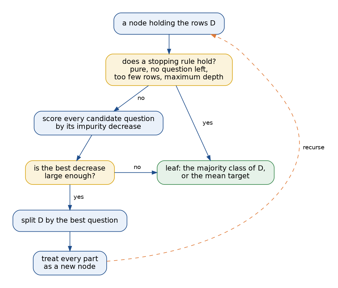
The flowchart is the whole algorithm. The two amber boxes are where the variants differ: which stopping rules apply, and how a question is scored. The dashed orange arrow is the recursion, which runs once for every part of every split.

Three ideas carry the rest of the page:

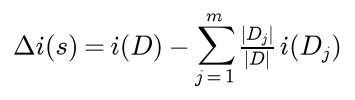
• Purity has to be measured. Entropy, the Gini index and the misclassification rate each turn the class shares of a node into one number that is zero for a pure node and largest for an even mix. The impurity decrease of a question is the impurity of the node minus the size-weighted impurity of its parts. With entropy this decrease is the information gain, the number of bits the answer reveals about the label.
• The search is greedy. The best question is chosen one node at a time and never revisited. Finding the smallest tree consistent with the data is NP-complete, so every practical algorithm settles for this greedy search, and a slightly different sample of the data can send it down a different path.
• A tree carves the feature space into rectangles. Every question tests one feature against one value, so every leaf is an axis-aligned box and the prediction is constant inside it. A deep tree can draw any boundary, including one around every noisy training point; controlling that freedom by stopping early or by pruning afterwards is what makes a tree generalize.

Three classic algorithms differ in the details:

• ID3 splits a categorical attribute into one branch per value and chooses by information gain. It does not handle numeric features, which must be discretized first, has no treatment of missing values, does no pruning and only classifies.
• C4.5 keeps the one-branch-per-value splits, adds binary thresholds for numeric features, chooses by gain ratio, sends rows with a missing value down every branch with fractional weights, and prunes by an error estimate.
• CART makes every split binary: a threshold for a numeric feature, a subset of the values for a categorical attribute. It chooses by the Gini index for classes and the squared error for numbers, so it also builds regression trees, replaces missing values with surrogate splits and prunes by cost complexity.

scikit-learn implements an optimized version of CART that takes numeric features only.

How it works

Notation

The formula images use subscripts; the text writes the same quantities in words, and writes DL, nL or SR where a formula has a subscript L or R.

• D is the set of training rows that reach a node and n their number. K is the number of classes and pk the share of rows of class k in D.
• A is a categorical attribute and v one of its values. Dv holds the rows of D whose value of A is v, and wv is their share of D. The share of class k among those rows is written p with indices k and v.
• H(D) is the entropy of the class shares in D and H(D | A) the conditional entropy after splitting on A, both in bits. IG, SI and GR are the information gain, the split information and the gain ratio.
• G(D) is the Gini index, E(D) the misclassification error and i(D) any impurity measure.
• A numeric feature xj is split at a threshold θ into the left part DL, the rows with the feature at most θ, and the right part DR.
• T is a tree, and the set of its leaves is written T with a tilde, so the vertical bars around it count the leaves. For a node t, Tt is the branch below t with t as its root, nt is the number of training rows that reach t and N the number at the root.
• R(t) is the weighted impurity of a node, its impurity times its share nt/N of the training rows, and R(T) the sum of R over the leaves of T. α is the complexity parameter of cost-complexity pruning.

The generic tree-induction algorithm

All the algorithms above follow the procedure of the flowchart. Called on the rows D of a node with a list of usable attributes:

1. If a stopping rule holds, return a leaf that predicts the majority class of D, or the mean of the target for regression. The rules that always apply are that every row has the same class, that no usable attribute is left, or that all rows have identical features. Pre-pruning adds more, such as a maximum depth or a minimum number of rows.
2. For every candidate split s of D into parts D1 to Dm, compute the impurity decrease below.
3. Take the split with the largest decrease. If the decrease is below a threshold, return a leaf instead.
4. For every part of the chosen split, grow a child: a leaf with the majority class of D if the part is empty, otherwise the result of calling the procedure on the part. A categorical attribute split into one branch per value is removed from the list passed to the children, because it is constant inside each branch and has nothing more to say there; a numeric feature stays, since it can be split again at another threshold.
5. Return a node that tests the chosen split and points to the children.

A new example is classified by starting at the root, following the branch that matches its value at every node and reporting the leaf's prediction. A value that never occurred at a node during training has no branch; the usual remedy, used here, is to stop there and report the majority class of that node.

Entropy and conditional entropy

The entropy of the class shares of a node, in bits, is

It is 0 when one class has all the rows and largest, log₂ K, when all classes are equally common; for two classes it peaks at one bit. Information theory derives it as the average number of yes-or-no questions needed to name the class of a random row. After a split on A, each branch has its own entropy, and the conditional entropy is their average weighted by branch size:

Each branch contributes in proportion to how many rows it holds, so a tiny pure branch earns little credit and a large mixed one costs a lot.

Information gain, and why it is never negative

The information gain of A is the drop in entropy:

It is the mutual information between the attribute and the label, computed from the rows in D: the number of bits that knowing A saves, on average, in describing the label. ID3 splits on the attribute with the largest gain.

The gain cannot be negative. Every row of class k lies in exactly one branch, so the class shares of the parent are the size-weighted average of the class shares of the branches:

Entropy is a concave function of the vector of class shares: its second derivatives are minus 1/(pk ln 2) on the diagonal and zero elsewhere. For a concave function the value at an average is at least the average of the values, which is Jensen's inequality. Writing the bold p with index v for the vector of class shares in branch v:

Entropy is strictly concave, so equality holds only when every branch has exactly the parent's class shares. A split whose branches have nearly the parent's shares therefore has a gain close to zero, however different the branch entropies may look written side by side.

Many-valued attributes and the gain ratio

The same argument applied inside each branch shows that refining a split never lowers its gain. If attribute B refines A, meaning every value of B occurs together with only one value of A, each branch of A is the union of some branches of B, Jensen's inequality applies within it, and B gains at least as much as A. An identifier column, with a different value on every row, refines every other attribute. Each of its branches holds one row and is pure:

That is the largest gain any attribute can have. The tree that splits on it memorizes the training rows and predicts nothing about a new one.

The bias does not need an identifier. If an attribute with m values is independent of the label, its gain on n rows is still positive on average, because the class shares of small branches fluctuate. The statistic 2 n ln 2 times the gain is the likelihood-ratio statistic for independence of A and the label, and under independence it is approximately chi-squared with (m - 1)(K - 1) degrees of freedom, so

The expected gain of pure noise grows linearly with the number of values: for two classes and 200 rows, 0.0036 bits for a binary attribute and 0.0685 bits for one with 20 values. The approximation underestimates once the branches hold only a few rows each.

Quinlan's correction divides the gain by the entropy of the branch sizes, the split information:

The split information measures how finely A cuts the rows, regardless of the labels. It is at most log₂ m, and for an identifier it is log₂ n, which gives the identifier a gain ratio of H(D) divided by log₂ n. That shrinks only slowly with n, so on small data the identifier can still win, as the Pitfalls section shows. Gain ratio has a bias of its own: an attribute that puts almost every row in one branch has a split information close to zero and a huge ratio. C4.5 therefore chooses by gain ratio only among the attributes whose gain is at least the average gain.

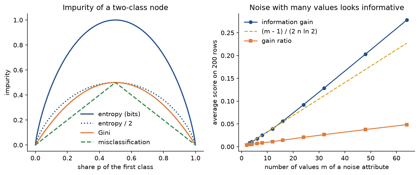
The left panel compares the impurity measures, discussed next. The right panel averages 300 draws of a noise attribute with m equally likely values and random labels: the gain follows the approximation closely up to about 16 values and then rises faster, while the gain ratio grows far more slowly. examples/impurity_measures.py draws it.

Gini impurity and the misclassification error

CART measures impurity with the Gini index:

It is the probability that two rows drawn at random with replacement belong to different classes, and also the error rate of a rule that guesses class k with probability pk. Like entropy it is zero for a pure node, largest for an even mix (1 - 1/K, so 0.5 for two classes) and strictly concave, so the Gini decrease is never negative either. The two are close relatives. Since minus ln p is at least 1 - p for p between 0 and 1, with equality at p = 1,

The Gini index is the first-order approximation of entropy measured in nats. For two classes, half the entropy in bits and the Gini index lie close together, as the left panel above shows, and the two criteria choose the same split in the large majority of cases. Gini avoids the logarithm, which made it cheaper on old hardware; entropy penalizes nearly pure nodes a little more.

The misclassification error is the training error of predicting the majority class. It is concave but not strictly, and that makes it a poor split criterion. If the same class k* is the majority in the parent and in every branch, then

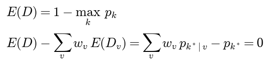
The split makes no progress by this measure, however much purer its branches are. Growing with the misclassification error stalls on splits that would enable good splits below them. It is a fine measure for judging a finished tree and for pruning.

Numeric features and threshold search

A numeric feature is split by a threshold:

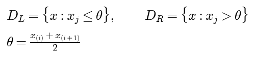
Only the order of the values matters, so only n - 1 thresholds can give different splits: sort the values of the node and place a candidate halfway between every two consecutive distinct values. The class counts on the left of each candidate are cumulative sums along the sorted order, so all candidates of one feature are scored in one pass after a sort that costs about n log n steps, and a node with p features costs about p n log n.

Not even every candidate needs scoring. Call a candidate a boundary point if the rows just below and just above it have different classes. Fayyad and Irani proved that the threshold with the smallest weighted entropy is always a boundary point: inside a run of rows of one class, the weighted entropy as a function of the cut position is concave, so it is smallest at one end of the run. The same holds for the Gini index. Because only the order matters, a tree is unchanged by any strictly increasing transformation of a feature, such as a change of units or a logarithm. Trees need no feature scaling.

CART: binary splits

CART splits every node in two. For a numeric feature that is a threshold. For a categorical attribute with m values it is a subset of the values sent left, and there are 2ᵐ⁻¹ - 1 such subsets. For two classes, and for regression with the squared error, a theorem of Breiman and colleagues, going back to Fisher for regression, removes the exponential search: sort the values by the share of class 1 among their rows, or by their mean target, and the best subset is one of the m - 1 splits of that ordering. Any multiway split can be written as a sequence of binary splits, so binary trees lose no expressive power; they fragment the data more slowly and the many-values bias is weaker, though a numeric feature with many distinct values still offers many candidate thresholds.

Regression trees and variance reduction

For a numeric target a leaf predicts the mean of its rows, the constant that minimizes the squared error, and the impurity of a node is the mean squared deviation from that mean, its variance:

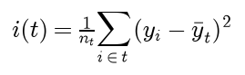
The impurity decrease of a split into L and R is the variance reduction, and it has a closed form. Split the total sum of squares of the node into the parts within and between the two groups, the first line below. The mean of the node is the size-weighted average of the two group means, which gives the differences in the second line. Substituting them makes the between-group term nL nR / nt times the squared difference of the means, and dividing by nt gives the third line:

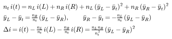
The best split separates the two means as far as possible, weighted by how balanced the split is. Writing SL and SR for the sums of the targets on each side and S for their total, and using the fact that n times the variance is the sum of squares minus S²/n, the same decrease becomes

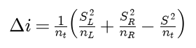
so the search only has to maximize SL²/nL + SR²/nR, which cumulative sums deliver for every threshold in one pass.

Stopping rules and pre-pruning

A tree grown until every leaf is pure fits the training rows perfectly, noise included. Pre-pruning stops earlier. In scikit-learn the rules are:

• max_depth, the deepest level a node may have;
• min_samples_split, so that a node with fewer rows becomes a leaf;
• min_samples_leaf, so that no split leaves fewer rows in a child;
• min_impurity_decrease, so that a split must lower the weighted impurity, its decrease times nt/N, by at least this much;
• max_leaf_nodes, which grows the tree best first and stops at this many leaves.

All of them suffer from the horizon effect: a split with little or no immediate decrease can enable very good splits below it. When the label is the exclusive or of two attributes, neither attribute alone changes the class shares, both gains at the root are exactly zero, and a rule that requires a positive gain never discovers that two levels separate the classes perfectly.

Cost-complexity pruning

Post-pruning grows the full tree first and then removes branches whose improvement is not worth their size. Cost-complexity pruning, from CART, scores a tree by its total weighted leaf impurity plus a price α per leaf:

Consider an internal node t. Collapsing the branch below it into the single leaf t changes the cost-complexity by

which is zero at the effective α of the node,

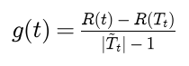
and negative for any larger α. R(t) is at least the R of its branch because impurity decreases are never negative, so g(t) is never negative. The node with the smallest g(t) is the weakest link: the branch that buys the least impurity reduction per extra leaf. Weakest-link pruning collapses it, updates the branch impurities and leaf counts of its ancestors, and repeats until only the root is left. This produces a nested sequence of trees T0, T1 and so on down to the root alone, with increasing values α0 = 0, α1, α2 and so on, and Breiman and colleagues proved that for every α from αk up to but excluding αk+1, the tree Tk is the smallest subtree of the full tree that minimizes the cost-complexity. The whole family of optimal pruned trees is found in one pass, and α is chosen by cross-validation over the values αk. A single round can collapse a branch with several splits at once, so the sequence can skip sizes.

scikit-learn computes R(t) with the training criterion, Gini, entropy or squared error, prunes every node whose g(t) is at most ccp_alpha, and returns the values αk and the total leaf impurities from cost_complexity_pruning_path. The original CART book uses the training misclassification rate for classification trees instead.

Missing values

Several approaches exist; in short:

• C4.5 computes the gain on the rows whose value is known and scales it by their share. A row with a missing value is sent down every branch with a weight proportional to the branch sizes, and at prediction time the class distributions of all the leaves it reaches are combined with those weights.
• CART keeps at every node a list of surrogate splits on other features that best reproduce the primary split, and uses the first one whose feature is present.
• scikit-learn, from version 1.3 with the default splitter, tries the rows with a missing value on both sides of every candidate split and keeps the side with the larger decrease. At prediction time missing values follow that side, or go to the larger child if the feature had no missing values during training.
• Imputing inside a pipeline, optionally with an indicator column for missingness, works with any tree implementation. The implementation on this page expects complete data.

Feature importance

The impurity importance of feature j, also called the mean decrease in impurity, adds up the weighted decreases of the nodes that split on it, and the results are normalized to sum to one:

It is free to compute but biased. It is measured on the training rows, every split counts as a decrease even when it only fits noise, and a feature with more distinct values offers more candidate thresholds and therefore more chances to fit noise, so continuous and high-cardinality features collect importance they do not deserve, most of all in deep trees. Permutation importance, the drop in a score on held-out rows when one column is shuffled, measures how much the model relies on a feature for new data and does not have this bias.

Decision boundaries

Each node tests one feature against one threshold, so the set of points that reach a leaf is the intersection of the half-spaces along its path, an axis-aligned box with some bounds possibly infinite:

The leaves tile the feature space and the prediction is constant on each tile. A boundary that is not aligned with the axes, such as the diagonal where the two features add up to zero, can only be approximated by a staircase of boxes, which needs many leaves and many rows.

Worked example

Sixteen tickets from a help desk. Each has a ticket number, the channel it arrived through, its priority, its category and the customer's plan, and the label says whether it was resolved on the day it arrived. Listed as number: channel, priority, category, plan, outcome:

• T01: email, high, billing, premium, yes.
• T02: email, high, billing, basic, yes.
• T03: phone, high, account, premium, no.
• T04: phone, high, technical, premium, no.
• T05: chat, high, account, premium, yes.
• T06: chat, high, account, premium, yes.
• T07: phone, low, account, premium, no.
• T08: email, low, billing, basic, no.
• T09: phone, low, billing, basic, yes.
• T10: chat, high, billing, premium, yes.
• T11: phone, low, technical, premium, no.
• T12: chat, low, billing, basic, yes.
• T13: email, low, account, premium, no.
• T14: chat, high, billing, premium, yes.
• T15: email, low, technical, premium, no.
• T16: phone, high, technical, basic, no.

Every value below is computed in double precision and shown to four decimals; values that are exact with five decimals are shown exactly. Sums written out from rounded terms can differ from the full-precision result in the last digit, and the text says where that happens. Class counts are written yes/no.

The root node

Eight tickets were resolved the same day and eight were not, so H(D) = 1 bit. A branch with 2 yes and 3 no has entropy 0.4 × log₂(5/2) + 0.6 × log₂(5/3) = 0.4 × 1.3219 + 0.6 × 0.7370 = 0.5288 + 0.4422 = 0.9710, and one with 1 yes and 5 no has (1/6) log₂ 6 + (5/6) log₂(6/5) = 0.4308 + 0.2192 = 0.6500. Doing the same for every branch of every attribute:

• Channel: chat 5/0, email 2/3 and phone 1/5, with branch entropies 0, 0.9710 and 0.6500. The conditional entropy is 5/16 × 0 + 5/16 × 0.9710 + 6/16 × 0.6500 = 0.3034 + 0.2438 = 0.5472, and the gain 0.4528.
• Priority: high 6/3 and low 2/5, with entropies 0.9183 and 0.8631. The conditional entropy is 9/16 × 0.9183 + 7/16 × 0.8631 = 0.5165 + 0.3776, which is 0.8941 from the rounded terms and 0.8942 at full precision, and the gain 0.1058.
• Category: account 2/3, billing 6/1 and technical 0/4, with entropies 0.9710, 0.5917 and 0. The conditional entropy is 5/16 × 0.9710 + 7/16 × 0.5917 = 0.3034 + 0.2589 = 0.5623, and the gain 0.4377.
• Plan: basic 3/2 and premium 5/6, with entropies 0.9710 and 0.9940. The conditional entropy is 0.9868 and the gain 0.0132.

Channel wins with a gain of 0.4528 bits, ahead of category by 0.0151. Plan deserves a second look. Three of five basic tickets were resolved against five of eleven premium ones, which looks like a difference, but both branches are close to an even mix, close to the parent's shares, and the gain is 0.0132 bits: almost nothing, exactly as the Jensen argument predicts.

The ticket number and the gain ratio

The ticket number puts each ticket in a branch of its own. Every branch is pure, the conditional entropy is 0 and the gain is the full bit, more than any real attribute. ID3 with the ticket number among its attributes splits on it at the root and stops with sixteen leaves, a lookup table of the training set. The gain ratio divides by the split information, the entropy of the branch sizes. For channel it is 2 × (5/16) log₂(16/5) + (6/16) log₂(16/6) = 2 × 0.5244 + 0.5306 = 1.5794 bits. In full:

• Ticket number: sixteen branches of one row, split information 4, gain 1, gain ratio 0.25.
• Channel: branch sizes 5, 5 and 6, split information 1.5794, gain ratio 0.4528 / 1.5794 = 0.2867.
• Category: sizes 5, 7 and 4, split information 1.5462, gain ratio 0.2831.
• Priority: sizes 9 and 7, split information 0.9887, gain ratio 0.1071.
• Plan: sizes 5 and 11, split information 0.8960, gain ratio 0.0147.

The ticket number needs log₂ 16 = 4 bits of split information, so its gain ratio is 1/4, below channel and category, and a tree grown by gain ratio ignores it and ends up with the same six leaves as the ID3 tree below. The margin is not large, though: the Pitfalls section shows the ticket number winning on ten tickets.

Gini and the misclassification error on the same splits

The root has Gini 1 - (0.5² + 0.5²) = 0.5. The email branch has 1 - (0.4² + 0.6²) = 0.48 and the phone branch 1 - (1/36 + 25/36) = 0.2778, so channel leaves 5/16 × 0.48 + 6/16 × 0.2778 = 0.15 + 0.1042 = 0.2542. The misclassification error counts the tickets that the majority of their branch gets wrong: channel and category each get 3 of 16 wrong, against 8 of 16 at the root.

• Channel: branch Gini 0, 0.4800 and 0.2778, weighted 0.2542, Gini decrease 0.2458, error decrease 0.3125.
• Priority: branch Gini 0.4444 and 0.4082, weighted 0.4286, Gini decrease 0.0714, error decrease 0.1875.
• Category: branch Gini 0.4800, 0.2449 and 0, weighted 0.2571, Gini decrease 0.2429, error decrease 0.3125.
• Plan: branch Gini 0.4800 and 0.4959, weighted 0.4909, Gini decrease 0.0091, error decrease 0.0625.

Gini ranks the four attributes exactly as entropy does, channel just ahead of category. The misclassification error cannot separate the two at all.

The email and phone nodes

The chat branch is pure, with 5 yes, and becomes a leaf. Channel is removed from the list, and the two impure branches are split on the remaining attributes.

The email tickets T01, T02, T08, T13 and T15 have 2 yes and 3 no, so their entropy is 0.9710:

• Priority: high 2/0 and low 0/3, conditional entropy 0, gain 0.9710.
• Category: account 0/1, billing 2/1 and technical 0/1, conditional entropy 3/5 × 0.9183 = 0.5510, gain 0.4200.
• Plan: basic 1/1 and premium 1/2, conditional entropy 2/5 × 1 + 3/5 × 0.9183 = 0.9510, gain 0.0200.

The phone tickets T03, T04, T07, T09, T11 and T16 have 1 yes and 5 no, so their entropy is 0.6500:

• Priority: high 0/3 and low 1/2, conditional entropy 3/6 × 0.9183 = 0.4591, gain 0.1909.
• Category: account 0/2, billing 1/0 and technical 0/3, conditional entropy 0, gain 0.6500.
• Plan: basic 1/1 and premium 0/4, conditional entropy 2/6 × 1 = 0.3333, gain 0.3167.

Priority splits the email tickets perfectly and category the phone tickets, so every leaf is pure and ID3 stops. The finished tree has six leaves and depth two:

Green leaves predict yes and orange leaves no. A new phone ticket about billing is predicted to be resolved the same day, a high-priority email ticket too whatever its category, and a phone ticket about an account is not.

Exact versus rounded logarithms

A calculation by hand often takes log₂ of whole numbers from a table rounded to one decimal, log₂ 3 ≈ 1.6, log₂ 5 ≈ 2.3, log₂ 6 ≈ 2.6 and log₂ 7 ≈ 2.8, and computes a branch entropy as log₂ n minus the count-weighted average of log₂ of the class counts. With that table the email branch has entropy 2.3 - (2 × 1 + 3 × 1.6)/5 = 0.94 instead of 0.9710, the phone branch 0.6833 instead of 0.6500, and the billing branch 2.8 - 6 × 2.6/7 = 0.5714 instead of 0.5917. The root gains become:

• Channel: 0.45 instead of 0.4528.
• Priority: 0.09375 instead of 0.1058.
• Category: 0.45625 instead of 0.4377.
• Plan: -0.00625 instead of 0.0132.

The table puts category first, and ID3 run with it grows a different tree with category at the root and eight leaves instead of six. It also gives the premium branch of plan an entropy of 1.0364 bits, more than the one-bit maximum for two classes, and plan a negative gain, both impossible. When two gains are this close, keep at least four significant digits in every logarithm.

A numeric feature: searching for a threshold

Eight tickets with the minutes until the first reply, sorted: 4, 9, 15, 22, 30, 41, 55 and 70 minutes, with outcomes yes, yes, yes, no, yes, no, no and yes. With 5 yes and 3 no the node has Gini 1 - (25 + 9)/64 = 0.46875 and entropy 0.9544. The seven candidate thresholds are the midpoints between neighbours:

• 6.5: left 1/0, right 4/3, Gini 0 and 0.4898, weighted 0.4286, Gini decrease 0.0402, entropy decrease 0.0924.
• 12: left 2/0, right 3/3, Gini 0 and 0.5, weighted 0.375, Gini decrease 0.09375, entropy decrease 0.2044.
• 18.5: left 3/0, right 2/3, Gini 0 and 0.48, weighted 0.3, Gini decrease 0.16875, entropy decrease 0.3476.
• 26: left 3/1, right 2/2, Gini 0.375 and 0.5, weighted 0.4375, Gini decrease 0.03125, entropy decrease 0.0488.
• 35.5: left 4/1, right 1/2, Gini 0.32 and 0.4444, weighted 0.3667, Gini decrease 0.1021, entropy decrease 0.1589.
• 48: left 4/2, right 1/1, Gini 0.4444 and 0.5, weighted 0.4583, Gini decrease 0.0104, entropy decrease 0.0157.
• 62.5: left 4/3, right 1/0, Gini 0.4898 and 0, weighted 0.4286, Gini decrease 0.0402, entropy decrease 0.0924.

For 18.5 the weighted Gini is 3/8 × 0 + 5/8 × 0.48 = 0.3 and the decrease 0.46875 - 0.3 = 0.16875. Both criteria choose 18.5. The boundary points, where the class changes between neighbours, are 18.5, 26, 35.5 and 62.5. The thresholds 6.5 and 12 lie inside the run of three yes and are beaten by 18.5 at its end; 48 lies inside the run of two no and is beaten by 35.5, as the boundary-point theorem promises.

A regression split

Six tickets with the number of messages exchanged and the hours until resolution: 1, 2, 4, 5, 7 and 9 messages took 3, 5, 4, 11, 14 and 12 hours. The mean is 49/6 = 8.1667 hours and the variance 511/6 - 8.1667² = 18.4722. The five thresholds:

• 1.5: left mean 3, right mean 9.2, variances 0 and 15.76, weighted 13.1333, decrease 5.3389.
• 3: left mean 4, right mean 10.25, variances 1 and 14.1875, weighted 9.7917, decrease 8.6806.
• 4.5: left mean 4, right mean 12.3333, variances 0.6667 and 1.5556, weighted 1.1111, decrease 17.3611.
• 6: left mean 5.75, right mean 13, variances 9.6875 and 1, weighted 6.7917, decrease 11.6806.
• 8: left mean 7.4, right mean 12, variances 18.64 and 0, weighted 15.5333, decrease 2.9389.

The split at 4.5 messages removes almost all the variance. The closed form gives the same decrease without computing any variance: (3 × 3 / 6²) × (4 - 12.3333)² = 0.25 × 69.4444 = 17.3611. The two leaves predict 4 and 12.3333 hours.

Cost-complexity pruning by hand

Grown until its leaves are pure, the CART tree on the first-reply data, with the Gini index, has four splits and five leaves. Each internal node has weighted impurity R(t) = (nt / 8) × G(t), and all leaves are pure, so the branch impurity below every node starts at zero.

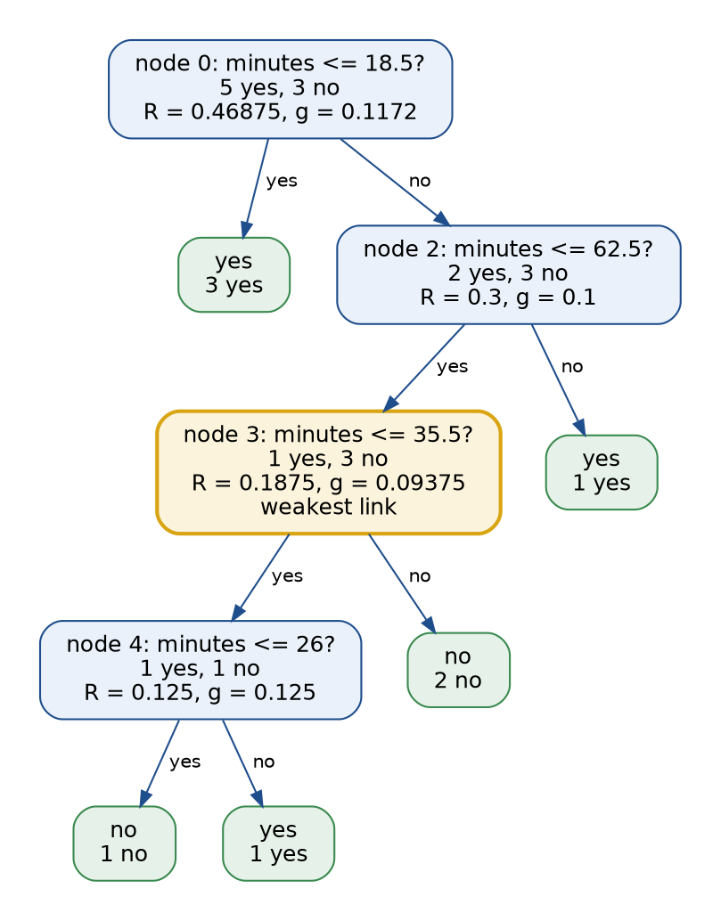
The diagram shows round 1 of weakest-link pruning, with the left branch of every test for yes. Every internal node carries its class counts, its weighted impurity R and its effective α, g, which is R divided by the number of leaves below it minus one:

• Node 0, the root, 5/3: R = 8/8 × 0.46875 = 0.46875, five leaves below, g = 0.46875 / 4 = 0.1172.
• Node 2, minutes above 18.5, 2/3: R = 5/8 × 0.48 = 0.3, four leaves, g = 0.3 / 3 = 0.1.
• Node 3, minutes from 18.5 to 62.5, 1/3: R = 4/8 × 0.375 = 0.1875, three leaves, g = 0.1875 / 2 = 0.09375.
• Node 4, minutes from 18.5 to 35.5, 1/1: R = 2/8 × 0.5 = 0.125, two leaves, g = 0.125.

The weakest link is node 3 at α1 = 0.09375. Collapsing it removes two splits at once, its own and the one at 26 below it, so the deepest split is not the first to go and the four-leaf tree never appears in the sequence. Three leaves remain, with total impurity 0.1875. In round 2 the root has g = (0.46875 - 0.1875)/(3 - 1) = 0.1406 and node 2 has g = (0.3 - 0.1875)/(2 - 1) = 0.1125, so node 2 is collapsed at α2 = 0.1125, leaving the single split at 18.5 with total impurity 0.3. In round 3 the root has g = (0.46875 - 0.3)/1 = 0.16875 = α3. The pruning path is:

• α0 = 0: total leaf impurity 0, five leaves.
• α1 = 0.09375: total leaf impurity 0.1875, three leaves.
• α2 = 0.1125: total leaf impurity 0.3, two leaves.
• α3 = 0.16875: total leaf impurity 0.46875, one leaf.

scikit-learn's cost_complexity_pruning_path returns exactly these numbers. Any ccp_alpha from 0.09375 up to but excluding 0.1125 gives the three-leaf tree. Every number in this section is asserted by the tests in tests/test_trace.py, tests/test_thresholds.py and tests/test_pruning.py, and printed by examples/worked_example.py and examples/thresholds_and_pruning.py.

The code

The package decision_trees is plain NumPy, split into one module per idea. scikit-learn is imported only inside the functions that load its data, split folds or fit its trees for comparison, and Matplotlib only by the drawing and plotting modules.

• arrays.py holds the array types and as_feature_matrix, which rounds features to 32-bit floats the way scikit-learn stores them.
• impurity.py holds entropy, gini, misclassification, rounded_log_entropy with a one-decimal logarithm table and variance, the measures collected in IMPURITIES.
• attributes.py scores a categorical split: score_attribute returns an AttributeScore with the branch counts, branch impurities, conditional impurity, gain, split information and gain ratio, and information_gain, gain_ratio and the other shortcuts compute one quantity each.
• id3.py holds grow_categorical_tree, ID3 with criterion="gain" or the gain-ratio variant with "gain_ratio", over any impurity measure, recording a NodeTrace for every node.
• trace.py holds ticket_tree and ticket_root_scores for the worked example and the formatters that print a build node by node.
• thresholds.py holds scan_thresholds, which scores every midpoint of one numeric feature for a class label or a numeric target, and between_group_reduction, the closed form of the variance reduction.
• tree.py holds the Tree class in scikit-learn's array layout, with apply, predict, predict_proba, impurity_decreases and feature_importances.
• splitting.py holds best_split, the vectorized threshold search, and cart.py holds grow_tree, CART for classification with Gini or entropy and for regression with the squared error, with max_depth, min_samples_split, min_samples_leaf and min_impurity_decrease.
• pruning.py holds weakest_link_pruning, which records every round, cost_complexity_path and prune.
• selection.py chooses the size of a tree: fold splits, cross_validated_accuracy, choose_alpha and depth_curve.
• regions.py holds leaf_rectangles, and evaluation.py holds accuracy, r2_score and permutation_importance.
• datasets.py holds the worked example's tables, the synthetic generators and breast_cancer_split.
• comparisons.py holds from_sklearn, which copies a fitted scikit-learn tree into a Tree, largest_difference and the library experiments of In practice.
• pitfalls.py and studies.py hold the experiments behind Pitfalls and the synthetic studies, and reports.py prints threshold scans, tree rules and pruning rounds.
• drawing.py draws a fitted tree with Matplotlib, and plotting.py, region_plots.py and palette.py draw every figure in the handbook's four colours.

grow_tree follows scikit-learn's choices closely enough to reproduce its trees: features are rounded to 32-bit floats before thresholds are computed, a threshold is the midpoint of two neighbouring values, nodes are numbered depth first with the left child first, and the split search maximizes the same proxy for the decrease. For one feature in a node, best_split sorts the rows, takes cumulative class counts and scores every admissible cut at once:

one_hot = np.zeros((count, n_classes))
one_hot[np.arange(count), ordered.astype(np.intp)] = 1.0
running = np.cumsum(one_hot, axis=0)
left = running[:-1]
right = running[-1] - left
impurity_left, impurity_right = node_impurities(criterion, left, n_left, right, n_right)
proxy = -n_right * impurity_right - n_left * impurity_left

Invalid cuts, between equal values or leaving fewer than min_samples_leaf rows on a side, get minus infinity, and the first maximum wins. Across features the lowest index wins ties; scikit-learn visits the features in a random order instead, which matters only when two splits are exactly equally good. The weakest-link loop computes g(t) for every remaining internal node, collapses the smallest and pushes the change up to the ancestors:

removed = n_leaves[chosen] - 1
difference = r_node[chosen] - r_branch[chosen]
node = parent[chosen]
while node != UNDEFINED:
    n_leaves[node] -= removed
    r_branch[node] += difference
    node = parent[node]

The examples and the project import the package, so install the repository first as described in the main README. The examples each demonstrate one idea and run in about a second from the repository root:

• examples/worked_example.py prints the categorical half of the worked example: the root scores under entropy, Gini and the misclassification error, the full ID3 trace, the identifier with and without gain ratio, and the tree grown with rounded logarithms.
• examples/thresholds_and_pruning.py prints the numeric half: both threshold scans, the regression split with its closed form, and the pruning rounds, checked against scikit-learn's path.
• examples/impurity_measures.py compares the impurity measures and measures the gain of noise attributes, and saves the figure under How it works.
• examples/depth_and_overfitting.py grows trees of every depth on noisy two-dimensional data, prunes the full tree by cross-validation, fits regression trees, and saves the three figures of In practice.
• examples/common_mistakes.py demonstrates each item of Pitfalls and saves its two figures.
• examples/compare_with_sklearn.py compares our trees with scikit-learn's node for node and shows ties, GridSearchCV and missing values in the library.

python machine-learning/decision-trees/examples/worked_example.py
python machine-learning/decision-trees/examples/thresholds_and_pruning.py
python machine-learning/decision-trees/examples/impurity_measures.py
python machine-learning/decision-trees/examples/depth_and_overfitting.py
python machine-learning/decision-trees/examples/common_mistakes.py
python machine-learning/decision-trees/examples/compare_with_sklearn.py

The sample project, project/pruned_tree_classifier.py, builds a small diagnostic model the way it should be built: grow a full tree, choose how far to prune it by cross-validation on the training part alone, and look at the test part once.

The diagram shows the flow of data. The test part, in orange, touches nothing until the final report, so the reported accuracy is an honest estimate.

The data are the Breast Cancer Wisconsin (Diagnostic) data: 569 tumours described by 30 measurements of cell nuclei from digitized images of fine-needle aspirates (the mean, standard error and worst value of ten quantities such as radius, texture and concavity), labelled malignant or benign. A stratified split keeps 171 tumours for testing. The full tree on the 398 training tumours has 16 leaves and depth 6, fits the training tumours perfectly and scores 0.9181 on the test tumours. Its pruning path has 12 values of α. Five-fold cross-validation repeated four times scores each one on 20 held-out parts; every fold tree is grown in full and pruned at every α. The best mean accuracy, 0.9303 with a standard error of 0.0065, belongs to α = 0.00879 and a tree with 6 leaves and depth 4, which scores 0.9181 on the test tumours, the same as the full tree with ten fewer leaves. It catches 56 of the 64 malignant test tumours and flags 6 of the 107 benign ones as malignant.

Options such as --criterion, --folds, --repeats, --test-size and --seed change the setup, and --figures sends the three PNGs to another folder so a custom run does not overwrite the ones shown here; the default run takes about two seconds.

python machine-learning/decision-trees/project/pruned_tree_classifier.py
python machine-learning/decision-trees/project/pruned_tree_classifier.py --criterion entropy

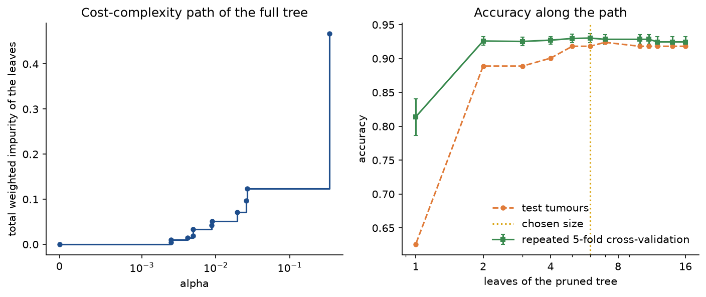
Across the path the cross-validated accuracy stays between 0.9246 and 0.9303 from 16 leaves down to 2, within about one standard error, while the test accuracy ranges from 0.8889 to 0.9240. On 171 test tumours one tumour is worth 0.0058, and differences of this size between pruning levels are noise.

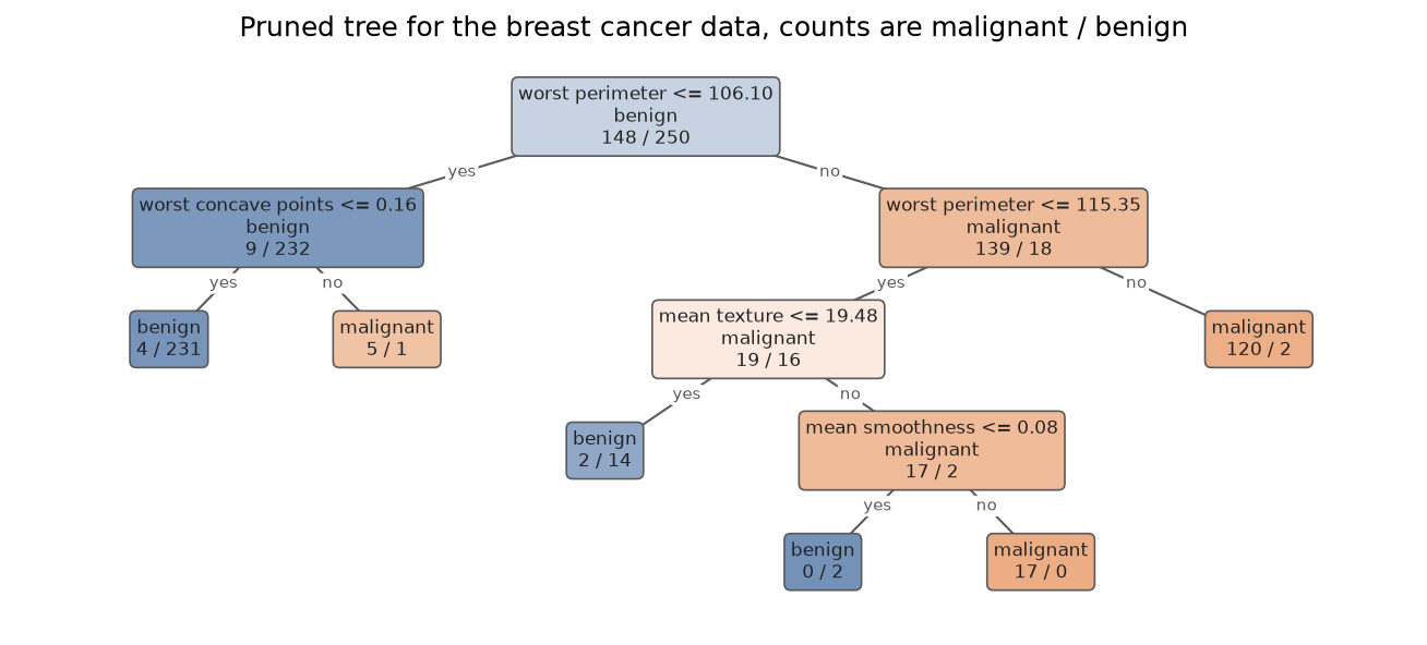
The pruned tree splits first on the worst perimeter at 106.10: below it, 232 of 241 training tumours are benign, and a worst concave points value above 0.16 picks out 5 of the 9 malignant ones; above 115.35, 120 of 122 are malignant. Orange boxes predict malignant and blue boxes benign, and the deeper the colour the purer the node.

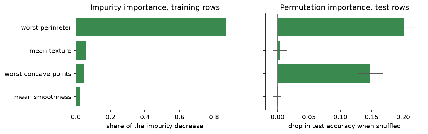
The two measures disagree about the second and third features. The impurity importances put 0.8718 on worst perimeter, 0.0609 on mean texture and 0.0461 on worst concave points; shuffling worst concave points on the test tumours costs 0.1476 in accuracy and shuffling mean texture only 0.0045. The impurity importance of the worst concave points split counts only the six training tumours it moves to the malignant side, but the tree relies on that feature for every small tumour: shuffled, the high values of malignant tumours land on small benign ones and send them to the malignant leaf.

The notebook decision_trees.ipynb is a guided tour in the order of this page: the ID3 trace and the identifier, rounded logarithms, threshold search, the regression split and the pruning rounds, then impurity measures, depth and pruning on synthetic data, each pitfall, the breast cancer tree and the comparison with scikit-learn. The tests in tests check the worked example value by value, the mathematical properties above and the agreement with scikit-learn, and run in about five seconds:

python -m pytest machine-learning/decision-trees

Every data set except one is synthetic and generated from a fixed seed by datasets.py. The breast cancer data, by W. H. Wolberg, W. N. Street and O. L. Mangasarian, come from the UCI Machine Learning Repository under the CC BY 4.0 licence and ship with scikit-learn as load_breast_cancer, so nothing is downloaded.

In practice

Agreement with scikit-learn

On data whose splits never tie, grow_tree builds the same tree as DecisionTreeClassifier and DecisionTreeRegressor: the same features, thresholds, sample counts, impurities and leaf values, node for node. On 400 rows of continuous random features the largest difference is 0 for a Gini tree of 27 nodes, 2 × 10⁻¹⁶ for an entropy tree of 25 nodes and 2 × 10⁻¹⁴ for a regression tree of 125 nodes; cost_complexity_path matches cost_complexity_pruning_path exactly, and the impurity importances agree with feature_importances_ to 10⁻¹⁴. Applied to a copy of scikit-learn's own full tree on the breast cancer training part, cost_complexity_path returns the identical path of 12 values, and prune returns, for every one of them, exactly the tree that DecisionTreeClassifier(ccp_alpha=...) fits. tests/test_comparisons.py asserts all of this, and examples/compare_with_sklearn.py prints it. In code, the library equivalent of the project is:

from sklearn.model_selection import GridSearchCV, RepeatedStratifiedKFold
from sklearn.tree import DecisionTreeClassifier

folds = RepeatedStratifiedKFold(n_splits=5, n_repeats=4, random_state=0)
tree = DecisionTreeClassifier(random_state=0)
path = tree.cost_complexity_pruning_path(features, labels)
search = GridSearchCV(tree, {"ccp_alpha": path.ccp_alphas}, cv=folds)
model = search.fit(features, labels).best_estimator_
model.tree_.feature, model.tree_.threshold, model.tree_.impurity, model.tree_.value

With the same folds, GridSearchCV chooses the same α = 0.00879, 6 leaves and test accuracy 0.9181. Its cross-validated accuracy is 0.9309 rather than 0.9303 because its fold trees break ties their own way, as explained below. tree_.value holds class shares for classifiers (older versions stored counts) and means for regressors, tree_.impurity the impurity of each node, and feature_importances_ the normalized impurity importance.

Overfitting and depth

examples/depth_and_overfitting.py grows CART trees on 300 points in the unit square, labelled by the side of a wavy curve they fall on, with 15 % of the labels flipped, so the best possible accuracy on fresh points is 0.8492. Training accuracy climbs to 1.0000 as the depth grows. Accuracy on 5,000 fresh points peaks at depth 3, with 8 leaves, at 0.8038, and falls to 0.7282 for the full tree with 59 leaves. Five-fold cross-validation on the training points tracks the fresh points, 0.8167 at depth 3 and 0.7333 at full depth, and picks the same depth. Pruning the full tree by cross-validation over its 29 path values chooses α = 0.01608 and four leaves, with fresh accuracy 0.7932.

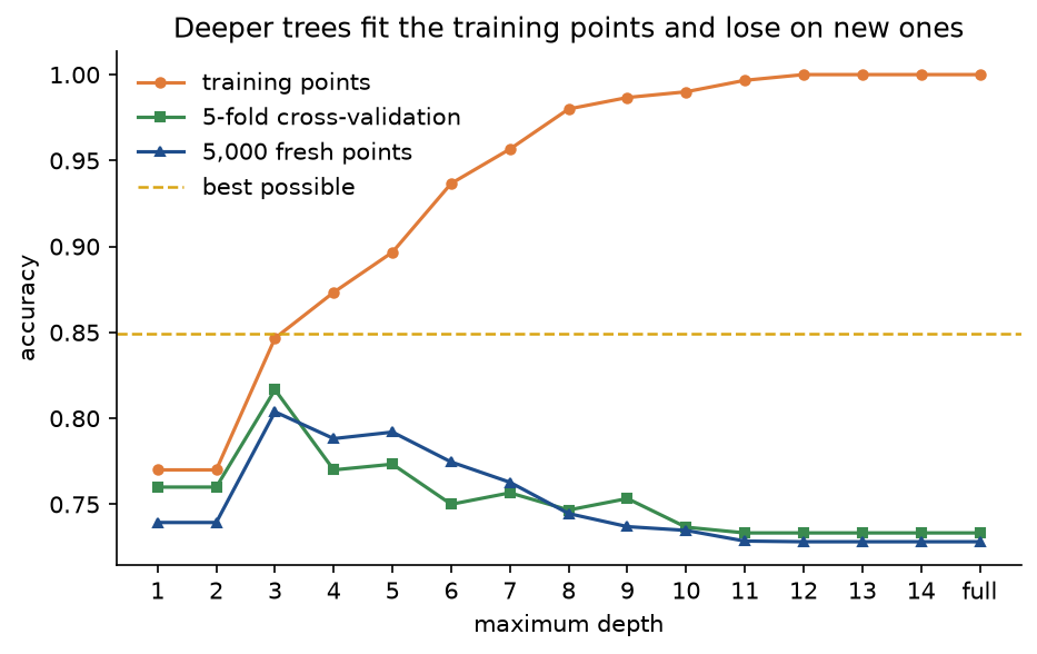
The gap between the training curve and the other two is the overfitting. Cross-validation needs no fresh data and still finds the right depth, which is why it is the tool for choosing a tree's size.

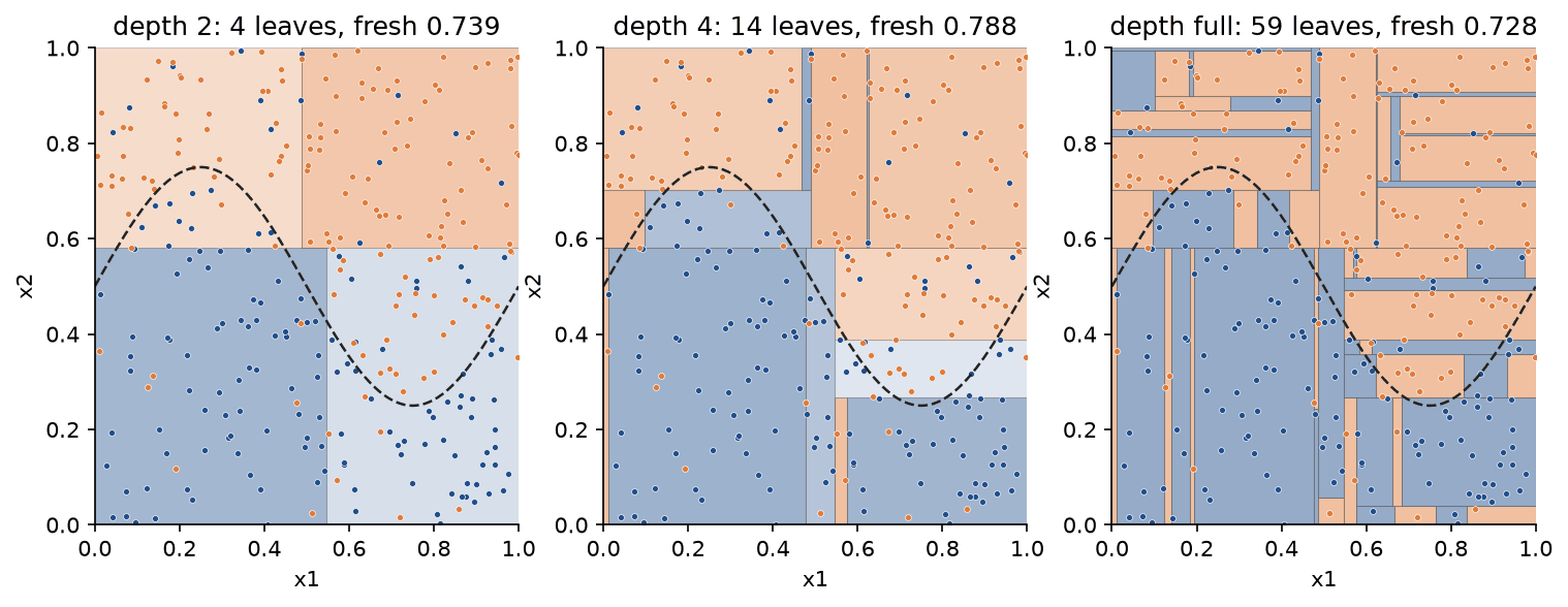
The decision regions are the leaf rectangles. At depth 2 four boxes approximate the curve crudely; at depth 4 fourteen boxes follow it; the full tree adds thin boxes around individual flipped points, each a region where a new point would be misclassified.

Regression trees

On 80 noisy points from a smooth curve, a regression tree of depth 1 has an R² of 0.6422 on 2,000 fresh points, depth 3 with 8 leaves reaches 0.8193, and the full tree with 80 leaves, one per point, drops to 0.7795 while scoring 1.0000 on its training points.

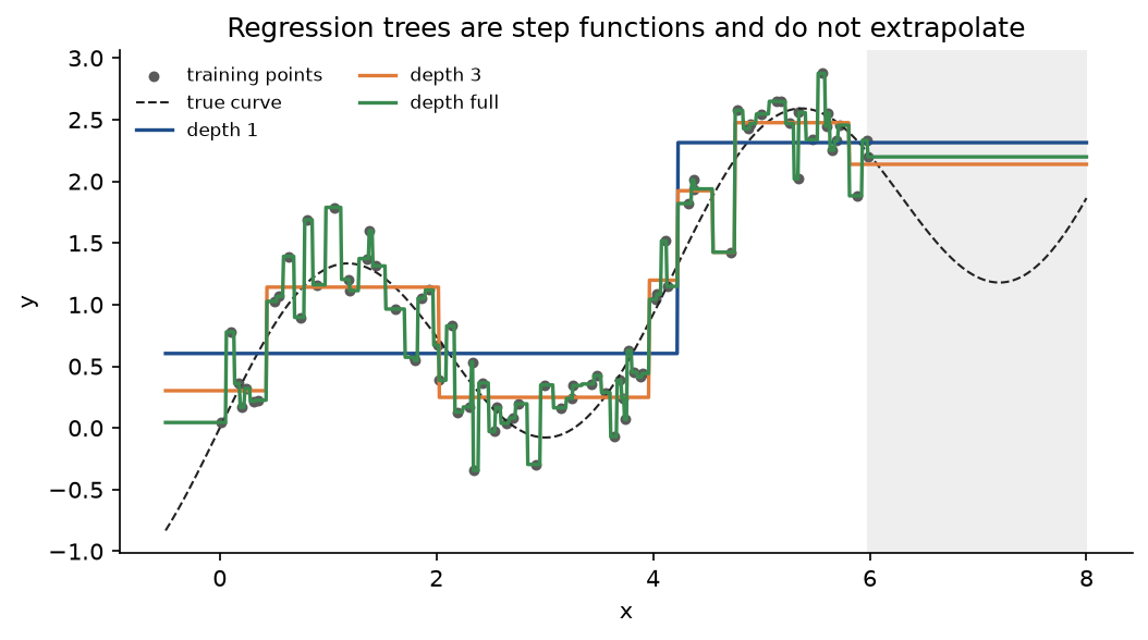
The fit is a step function, and beyond the last training point every tree predicts the constant of its last leaf, whatever the curve does there.

Ties and random_state

Even with every feature considered at every node, scikit-learn's trees depend on random_state, because the library visits the features in a random order and keeps the first of several equally good splits. Ties are common in small nodes, where several features separate the same few rows equally well: random_state 0 and 2 first differ at node 6, which holds 4 tumours, splitting on worst perimeter in one tree and on worst concavity in the other. Twenty values of random_state give twenty different full trees on the breast cancer training part, with 16 or 19 leaves and test accuracies from 0.8947 to 0.9357. grow_tree breaks ties by the lowest feature index and gives one more valid tree, with 16 leaves and 0.9181. Fix random_state to make a tree reproducible, and expect a different but equally good tree when it changes. A test can only demand agreement between implementations on data without ties, which is why the agreement tests use continuous random features.

Missing values in scikit-learn

When 20 % of the values of worst perimeter, the root feature, are removed from the training part, scikit-learn's tree simply splits on worst radius at 16.805 instead, an almost equivalent feature without gaps, much as a surrogate split would. On synthetic data where a value is missing five times as often for class 1, with 58 of 400 values missing, a one-split tree learns to send missing values to the class 1 side and predicts class 1 for a missing value. examples/compare_with_sklearn.py shows both.

When to use which

• Use the from-scratch code to see every number a tree is built from, to check a calculation by hand, and to experiment with criteria scikit-learn does not offer, such as gain ratio or multiway categorical splits.
• Use scikit-learn for real work. It is written in Cython, supports sample weights, missing values, monotonic constraints and best-first growth with max_leaf_nodes, and exposes the fitted arrays for inspection. Encode categorical attributes as numbers first: one-hot columns for nominal attributes, ordinal codes when the order means something.
• A single tree is the right model when it must be read and checked by people, as a set of rules, or as a fast baseline. Keep it small: choose ccp_alpha or max_depth by cross-validation, and report the spread across folds.
• When accuracy matters more than readability, average many trees. Trees have low bias and high variance, as the instability under Pitfalls makes plain, and Ensembles cancel the variance: bagging and random forests average trees grown on resampled data, and boosting adds small trees one after another.

Pitfalls

• Rounding logarithms early. Gains of competing attributes are often within a few hundredths of a bit. With log₂ rounded to one decimal, the worked example picks category instead of channel at the root, grows an eight-leaf tree instead of a six-leaf one, and assigns plan a negative gain and a branch an entropy above one bit, as examples/worked_example.py prints. A negative gain or an entropy above log₂ K is always an arithmetic error.
• Believing that gain ratio removes the identifier problem. It divides the identifier's gain by log₂ n, which grows slowly. On the first ten tickets alone the ticket number has a gain ratio of 0.2923 against 0.2361 for channel, so a gain-ratio tree would split on it. Drop identifiers, data-entry timestamps and other row-specific columns before growing a tree; Data leakage and pitfalls explains why such columns can also leak the label.
• Trusting the structure of one tree. Channel beats category at the root by 0.0151 bits. Leaving out a single ticket moves the root to category in 5 of 16 cases (T03, T05, T06, T07 or T08), produces an exact tie in 3 more (T10, T12 or T14, where the attribute listed first wins), and changes the number of leaves from 6 to as few as 4 or as many as 8. Small changes in the data change the tree, which is why the rules of a single tree are a poor explanation of the data and why ensembles exist. examples/common_mistakes.py prints every case.
• Reading impurity importance as relevance. With one weakly informative binary attribute and four noise attributes, full trees on 400 rows give the informative attribute an average impurity importance of 0.1513 over 20 draws, less than the noise with 10 values (0.1780), with 20 values (0.2161) and the continuous noise (0.3318). Permutation importance on 2,000 fresh rows gives the informative attribute 0.0714 and every noise attribute between -0.0016 and -0.0007. Use permutation importance on held-out data, and treat any impurity importance of a continuous or high-cardinality feature with suspicion.

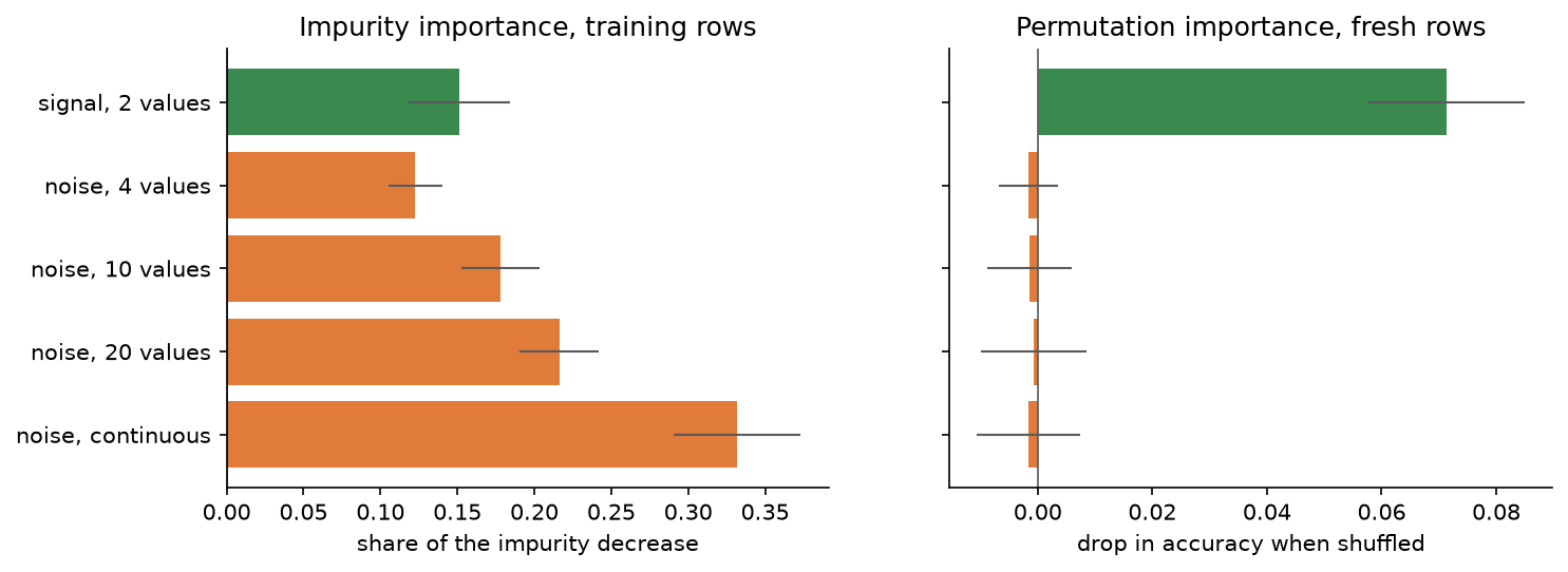
The left panel ranks the signal fourth of five; the right panel ranks it alone at the top, with the noise attributes indistinguishable from zero.

• Stopping as soon as the best gain is small. For the exclusive or of two attributes, both gains at the root are exactly zero. ID3 with a minimum gain of 0 returns a single leaf with training accuracy 0.50; grown one level further, the tree has four pure leaves. Prefer growing a large tree and pruning it to stopping on a threshold, and treat min_impurity_decrease as a hyperparameter to cross-validate.
• Splitting by the misclassification error. At the phone node every branch of priority and of plan keeps no as its majority, so the error does not drop at all, although the Gini decreases are 0.0556 and 0.1111 and the entropy decreases 0.1909 and 0.3167. At the root it ties channel with category. Grow with entropy or Gini; the error rate is for evaluating and pruning.
• Expecting trees to draw oblique boundaries. For classes separated by the diagonal where the two features add up to zero, a full tree on 400 points needs 22 leaves and depth 6 and scores 0.9562 on fresh points. On the rotated features u, the sum of the two features divided by √2, and v, their difference divided by √2, a single split scores 0.9998. Add sums, differences or ratios of features when domain knowledge suggests them, or use a model with linear boundaries.

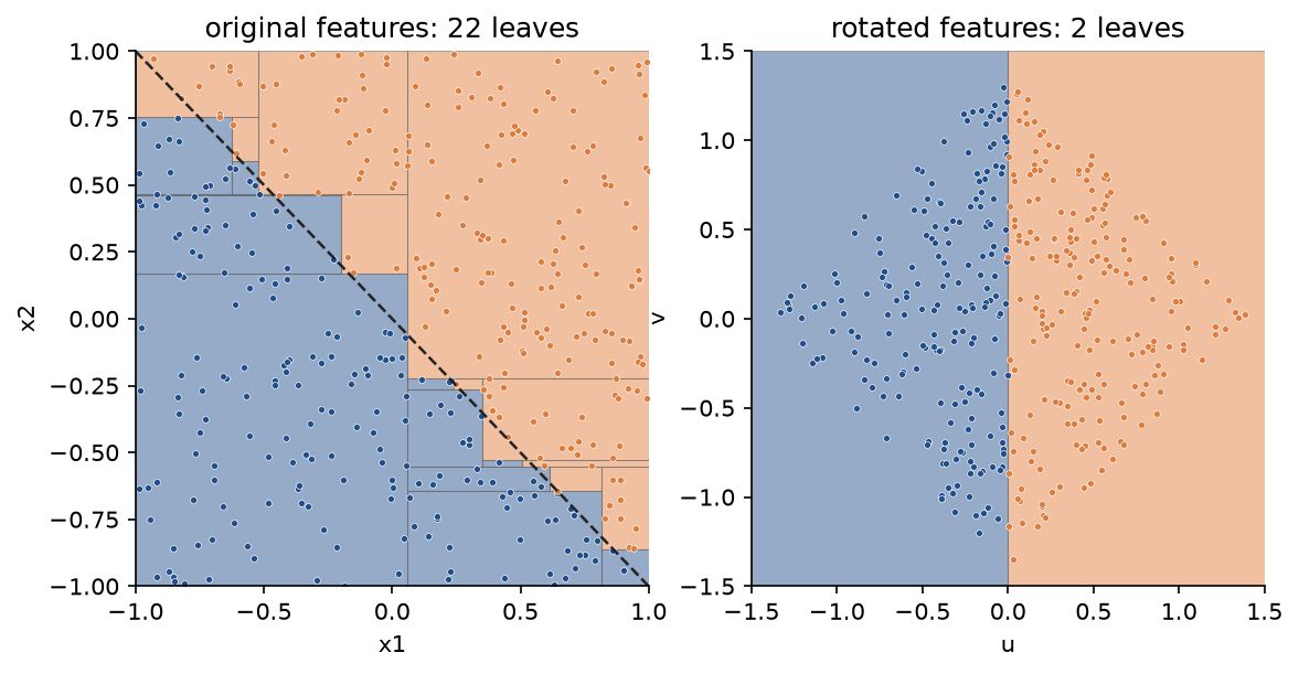
The staircase spends most of its leaves near the diagonal, where every step misclassifies a thin sliver of points; the rotation turns the same boundary into one axis-aligned cut.

• Extrapolating with a regression tree. Outside the range of the training data a regression tree predicts the constant of its last leaf, whatever the trend: a depth-4 tree on the noisy curve predicts 2.7081 at its last training input, 5.98, and the same at 10 and at 100. Do not use trees to forecast beyond the observed range of a feature that drives the target, such as time.
• Myths that come with the method. Trees do not need binary splits, since ID3 and C4.5 split categorical attributes many ways. They do not need feature scaling: rescaling every feature leaves every row in the same leaf, as examples/common_mistakes.py checks. They do not need balanced classes to work, although a minority class may need class weights to be found. They are robust to outliers in the features, because only the order of values matters, but not to outliers in a regression target: the squared error pulls a leaf's mean, and the variance criterion builds splits around the outlier.
• Choosing the depth or ccp_alpha on the test set. The test accuracy along the breast cancer path spans 3.5 points between 2 and 16 leaves while the cross-validated accuracy hardly moves; picking the size with the best test score reports noise as skill. Choose by cross-validation on the training part, as the project does, and look at the test set once.

Further reading

• J. R. Quinlan, "Induction of decision trees", Machine Learning 1(1), 81-106, 1986. ID3, information gain and the gain ratio.
• J. R. Quinlan, C4.5: Programs for Machine Learning, Morgan Kaufmann, 1993. Numeric thresholds, missing values and error-based pruning.
• L. Breiman, J. H. Friedman, R. A. Olshen and C. J. Stone, Classification and Regression Trees, Wadsworth, 1984. CART: binary splits, the Gini index, regression trees, surrogate splits and cost-complexity pruning with its optimality proof.
• L. Hyafil and R. L. Rivest, "Constructing optimal binary decision trees is NP-complete", Information Processing Letters 5(1), 15-17, 1976.
• U. M. Fayyad and K. B. Irani, "On the handling of continuous-valued attributes in decision tree generation", Machine Learning 8, 87-102, 1992. The boundary-point theorem.
• J. Mingers, "An empirical comparison of selection measures for decision-tree induction", Machine Learning 3, 319-342, 1989.
• L. E. Raileanu and K. Stoffel, "Theoretical comparison between the Gini index and information gain criteria", Annals of Mathematics and Artificial Intelligence 41, 77-93, 2004.
• C. Strobl, A.-L. Boulesteix, A. Zeileis and T. Hothorn, "Bias in random forest variable importance measures: illustrations, sources and a solution", BMC Bioinformatics 8, 25, 2007.
• T. Hothorn, K. Hornik and A. Zeileis, "Unbiased recursive partitioning: a conditional inference framework", Journal of Computational and Graphical Statistics 15(3), 651-674, 2006.
• T. Hastie, R. Tibshirani and J. Friedman, The Elements of Statistical Learning, second edition, Springer, 2009, section 9.2.
• W. N. Street, W. H. Wolberg and O. L. Mangasarian, "Nuclear feature extraction for breast tumor diagnosis", Proceedings of IS&T/SPIE Biomedical Image Processing and Biomedical Visualization, 1905, 861-870, 1993. The source of the breast cancer data.
• scikit-learn user guide, "Decision Trees" and the example "Post pruning decision trees with cost complexity pruning".